Abstract
Sensor faults can produce incorrect data and disrupt the operation of entire systems. In critical environments, such as healthcare, industrial automation, or autonomous platforms, these faults can lead to serious consequences if not detected early. This study explores how faults in MEMS microphones can be classified using lightweight ML models suitable for devices with limited resources. A dataset was created for this work, including both real faults (normal, clipping, stuck, and spikes) caused by issues like acoustic overload and undervoltage, and synthetic faults (drift and bias). The goal was to simulate a range of fault behaviors, from clear malfunctions to more subtle signal changes. Convolutional Neural Networks (CNNs) and hybrid models that use CNNs for feature extraction with classifiers like Decision Trees, Random Forest, MLP, Extremely Randomized Trees, and XGBoost, were evaluated based on accuracy, F1-score, inference time, and model size towards real-time use in embedded systems. Experiments showed that using 2-s windows improved accuracy and F1-scores. These findings help design ML solutions for sensor fault classification in resource-limited embedded systems and IoT applications.
1. Introduction
Sensors are one of the most important components of modern digital systems. With the rapid expansion of the Internet of Things (IoT), the use of sensors has increased significantly. Sensors enable the monitoring of real-time data and serve as a bridge between the physical world and digital processes. These devices capture and transmit real-time measurements. These measurements are then used for automation, system monitoring, control mechanisms, and predictive analytics. However, the reliability of sensor-based systems is directly dependent on the accuracy of the data collected by the sensors. The performance and data reliability of sensors may deteriorate over time due to challenging operating conditions such as electromagnetic interference, humidity, fluctuations in temperature, and mechanical or electrical stress [1]. These factors can lead to incorrect decision-making or even severe failures in critical applications such as healthcare systems, industrial automation infrastructures, and smart city environments. As observed in [2], sensor aging can pose critical risks and make sensors more vulnerable to attacks.
To prevent these types of risks, sensor fault detection has been an active research topic since the 1980s, aiming to ensure system reliability by identifying and addressing sensor-related problems early [3]. Fault detection refers to identifying whether a sensor is operating incorrectly, while fault classification is the process of determining the type of fault affecting the sensor’s performance [4].
In the literature, there are different methods used for sensor fault analysis, such as model-based, signal-based, and machine learning (ML)-based methods [5,6]. Model-based methods use mathematical or physical models to describe how a sensor should behave when everything is working normally. These methods check whether the actual sensor readings match what the model predicts. The difference between them is called the residual. Residual helps us to understand if something is wrong with the sensor. When the model is accurate, this method can detect faults very well. But building such a model often requires deep knowledge of the system and takes a lot of time and computing power. This can be a problem, especially for complex systems. Also, if the system changes suddenly or behaves in a non-linear way, the model may no longer be accurate, and the method might miss the fault [7]. Signal-based methods use a different approach. Instead of building a model, they look directly at the sensor signals. These methods use basic statistics like the average and variation to find anything unusual in the signal. They are simple, quick, and good for real-time use. But they can have problems catching small or slowly growing faults, especially if the signal has a lot of noise.
Recently, ML-based methods have become more popular because they can learn complex, non-linear patterns from large datasets. These methods learn from past data to recognize what normal and faulty signals look like. ML-based methods can achieve high accuracy and do not need a detailed model of the system. Because of their flexibility and strong performance, ML methods are now widely used for detecting sensor faults in real-world applications [5,8,9]. For these reasons, we also chose this approach in this work to classify sensor faults effectively.
In this study, MEMS (Micro-Electro-Mechanical Systems) microphones were used as the target sensors. Unlike simple sensors like temperature or humidity sensors, MEMS microphones produce complex and high-frequency audio signals. An audio signal is a form of time-series data that represents sound through rapid, detailed fluctuations in amplitude over time. These variations capture the full range of changes in a sound environment, making audio signals more complex to analyze than slower-changing data, such as temperature readings. MEMS microphones are widely used in embedded and consumer devices due to their small size, low cost, and good performance [10]. Studying faults in such sensors helps to develop solutions that can operate under more practical and demanding conditions.
Based on the discussed motivation, this research is guided by the following key points: First, it investigates whether lightweight ML models can classify sensor faults accurately while keeping memory usage and inference time low enough for use in resource-constrained devices. Second, it explores how the length of the input window impacts the accuracy and efficiency of the models. Third, it examines the effect of different sound categories (e.g., airplane, rain, alarms) on the classification performance of these models.
The main contributions of this work are as follows:
- A labeled fault dataset was created using MEMS microphone sensors, which, to the best of our knowledge, does not exist in the current literature. It includes both real faults, generated through acoustic overload and undervoltage conditions such as clipping, spike, stuck, and normal, and synthetic faults such as bias and drift.
- A sensor fault classification pipeline was developed using both deep learning and classical ML models. The impact of different window sizes (1 s and 2 s) on model performance, including accuracy, F1-score, inference time, and model size, was evaluated.
- A detailed experimental analysis was provided to support model selection for resource-constrained devices. The study also investigated how different sound categories, such as rain, alarms, and rivers, influence the ability to classify sensor faults.
This paper is structured as follows: Section 2 presents related studies on sensor fault detection and publicly available datasets. Section 3 describes the proposed methodology in detail. The experimental results are evaluated and discussed in Section 4. Finally, Section 5 concludes the paper and outlines potential directions for future work.
2. Related Work
Previous works based on ML have demonstrated significant potential in improving on fault detection and classification in sensor systems. Additionally, in this section, we also discuss the limitations of public datasets and highlight the gaps in existing studies.
2.1. Previous Works
Over the last years, the use of ML has been adopted to determine sensor faults. Umer Saeed et al. [11] proposed an ML-based implementation based on SVM, ANN, Naïve Bayes, KNN, and Decision Trees for real-time drift fault detection in humidity and temperature sensors. Their experimental results showed that SVM and ANN reached the best accuracy at 99%. The study exclusively focuses on drift faults and does not account for other potential sensor faults, limiting its scope to a single fault type in the current implementation.
An advanced method called the Context-Aware Fault Diagnostic framework was proposed in [5] to detect and diagnose sensor faults in healthy humidity and temperature sensors. They used a lightweight ML model based on the Extra Trees algorithm. In this study, they focused on six common fault types: drift, hard-over, spike, erratic, stuck, and data loss, leveraging contextual information such as hardware, communication, and calibration defects to improve diagnostic accuracy. They used a publicly available dataset [12] and synthetically injected sensor faults. The proposed study achieved an F1-score of 85.42% and a diagnostic accuracy of up to 90%, showing more efficient performance than SVM and NN.
Similarly, a sensor fault detection and prediction approach for autonomous vehicles was proposed in [13], utilizing SVM. The system has several steps. In the first step, it uses SVM to find potential sensor faults in real time. If a fault is detected, it identifies which sensor has the problem. Next, it classifies the type of fault (drift or spike). Finally, it predicts when a sensor might develop a fault. The system obtained a very high accuracy of 94.94 for fault detection, 97.42% for faulty sensor identification, 97.01% for classification of fault type, and 75.35% for prediction of erratic faults.
Different classifiers, including SVM, Random Forest, Stochastic Gradient Descent, MLP, CNN, and Probabilistic Neural Network, were evaluated for their classification performance in fault detection of temperature and humidity data in [14]. Offset, gain, stuck-at, spike, and data loss sensor faults were detected in temperature and humidity data measured by sensors over several time intervals. Random Forest achieved the best performance, with an F1-score of 93.15%, demonstrating strong results when the data were high-dimensional and the faulty instances were highly imbalanced.
Sensor fault detection and classification using SVM using statistical time-domain features was proposed in [15]. Five different sensor faults were considered: drift, hard-over, erratic, spike, and stuck. In order to obtain data, a temperature-to-voltage converter was used with an Arduino Uno board, and fault data were inserted by simulation. A number of features were used to observe the change in the accuracy of the SVM model, and the results showed that increasing the number of features from 5 to 10 changed the total accuracy only slightly. Three SVM kernels (linear, polynomial, and RBF) were compared, and the polynomial kernel delivered the best performance, with an overall accuracy of 91–93%. Similarly, an SVM-based approach for sensor fault detection in WSNs was proposed in [8], where labeled datasets derived from humidity and temperature measurements were used. In this study, the SVM classifier analyzed time-series features to distinguish between normal and faulty data. The solution provided a detection accuracy of 99% and above, showing better performance than Hidden Markov Models (HMMs) and Bayesian classifiers. Similarly, authors in [16] proposed an approach that employs HMMs to detect and classify faults within WSNs. This method models the relationship between fault-free and failed sensor states, addressing data faults (e.g., noise, spikes, gain, offset). With publicly available datasets (RUG Lab and Intel Lab), it achieved a detection accuracy of 95% and low false-positive and false-negative rates. However, HMMs are slow with large systems, assume fixed patterns in data, and struggle with long-term changes. This can make it harder to handle complex systems.
Combinations of ML techniques have also been proposed. Manhong Zhu et al. [17] presented an IoT sensor self-detection and self-diagnosis framework by combining Least Squares Support Vector Machines (LSSVMs) for anomaly detection with Decision Trees for fault classification. It begins with continuous monitoring of sensor outputs by LSSVM to identify any abnormal deviation in real time. Finally, after the detection of an abnormality, the feature extracted by wavelet packet decomposition determines the fault type with the help of decision trees. The proposed system achieved a 100% classification accuracy.
A real-time Edge AI solution for solar system fault detection was presented in [18]. They used a simple neural network model to detect different types of faults by utilizing data collected from solar systems. The model showed an accuracy of 97.84% and a size of 7.455 kB. This reduced model was implemented on different edge AI platforms, and STM32F767 Nucleo-144 (STMicroelectronics NV, Geneva, Switzerland) demonstrated the most cost-effective and energy-efficient performance.
A two-stage hybrid deep learning model for sensor fault detection and classification is presented in [1]. In the first stage, a CNN-LSTM model is trained on historical non-faulty sensor data, where the CNN is used for feature extraction and the LSTM predicts the future values of sensor readings. In the second stage, a CNN-MLP model is trained on fault-injected data to classify these forecasted values into one of several fault types. The model achieved high forecasting accuracy with an MAE of 2.0957 and a fault classification accuracy of 98.21%. Similarly, in [19], the authors proposed a two-stage method for finding malfunctioning sensors in a large network of air quality monitoring. In the first stage, several supervised learning models like Ridge Regression, Lasso Regression, Random Forest, Fully Connected Neural Networks, and LSTM are used to predict future PM2.5 values based on both spatial and temporal features from the sensor and five closest sensors. The second step involves residual analysis, which compares the predicted value with the actual value of PM2.5 to determine which sensors have the largest difference and are selected as faulty. LSTM showed the best performance among all models, achieving the highest accuracy with an AUROC score of 0.91. However, this proposed model does not classify the different types of sensor faults, which limits its ability to provide detailed fault diagnosis.
Sinha et al. [20] proposed a novel hybrid deep learning approach that isolates and classifies both sensor and machine faults using vibration data from induction motors. A CNN-XGBoost model is used for feature extraction and classification, while a denoising autoencoder reconstructs faulty sensor data to prevent misdiagnosis. The proposed model uses a CNN to extract features from the raw time-series data and then feeds them into an XGBoost model for classification. It classifies four sensor faults: bias, drift, precision degradation and complete failure. It achieved 98.15% accuracy for fault isolation and 99.77% for machine fault detection.
Existing studies mostly focused on sensors with slow variation (temperature, humidity, luminosity, …) while most of the sensors present fast data rate acquisition. Moreover, according to existing research, there is a clear gap in evaluating ML models for resource-constrained devices in terms of model size and latency. In this study, we addressed this issue by measuring and analyzing the efficiency of the models to ensure their suitability for resource-constrained devices.
2.2. Public Datasets
In the literature, two public datasets are commonly used for developing and evaluating sensor fault detection models.
- Intel Berkeley Research Lab Dataset: Several studies have adapted the Intel Berkeley Research Lab dataset [21] for their research. The original dataset consists of data from 54 sensors, including timestamped measurements of humidity, temperature, light, and voltage, collected every 31 s. It contains approximately 2.3 million samples. The original dataset is not labeled and does not include any fault types.
- Labeled Wireless Sensor Network Data Repository (LWSNDR): Suthaharan et al. [12] implemented a single-hop and multi-hop sensor network dataset using TelosB motes. The dataset consists of humidity and temperature measurements collected over a 6-h period at intervals of 5 s. This dataset is labeled as faulty or non-faulty. Several studies used this dataset by injecting different fault types.
2.3. Limitations and Research Gaps
Public datasets are often used in sensor fault studies, but they have some limitations. First, they mostly include data from simple sensors such as temperature and humidity sensors. These types of sensors produce slow-changing values that are easier to analyze and predict. However, in real applications, more complex sensors are often used. These sensors can generate fast, detailed, and more complicated signals. Another important issue is that the faults in these datasets are synthetic. Synthetic faults are faults added to the sensor data using mathematical patterns. Real faults occur during actual operation and result from real-world conditions such as hardware failures, signal interference, or environmental changes. These faults are usually more irregular, unpredictable, and complicated, making them harder to detect and classify. Because of this, publicly available datasets do not reflect the full complexity of real sensor faults. For these reasons, we decided to collect our own dataset and inject real faults into it, so we could train and evaluate fault classification models under more practical and challenging conditions.
In Table 1, detailed usage of the Intel Lab and LWSNDR datasets in various studies is provided.

Table 1.
Details of Intel Lab and LWSNDR dataset usage in various studies, including publication year and sensor type.
3. Methodology
The complete approach is structured into several stages, beginning with fault characterization of a MEMS microphone sensor using chirp signals under controlled conditions, including under-voltage and acoustic overload tests. Based on this, both real and synthetic faults are injected into clean recordings to build the dataset. After that, the data are subjected to preprocessing steps, followed by training AI models to classify the faults. A dedicated window size analysis is also conducted to compare the impact of 1 s vs. 2 s windows on classification performance. Evaluation included three scopes—only real faults, the full dataset, and per-category analysis (e.g., airplane, applause, birds)—to understand the model’s behavior across different sound types. A visual summary of the process is demonstrated in Figure 1. Each of these steps is detailed in the following subsections. The final stage, which is the window analysis of experimental results, is presented and discussed in Section 4.
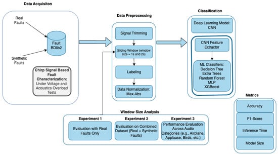
Figure 1.
Methodology for MEMS microphone sensor fault classification, including data acquisition, data preprocessing, and classification using standalone CNN and hybrid CNN+ML models. Three experiments are conducted with different window sizes. Metrics include accuracy, F1-score, inference time, and model size.
3.1. Experimental Setup
The experimental setup was specifically designed to investigate how MEMS microphones respond to both electrical and acoustic stress, while also enabling the collection of reliable audio data for our study. As illustrated in Figure 2, the system includes the following components: SPH0645 I2S MEMS microphones, an ESP32 Wemos microcontroller, a programmable DC power supply (RSPD 3303X-E), a speaker (Avantone MixCube), a QSC CX168 professional amplifier, a Norsonic Nor140 precision sound analyzer (Norsonic AS, Tranby, Norway), and a host computer. In this study, we used the SPH0645 MEMS microphone sensor. This sensor provides low power consumption, high sensitivity, and the capability to capture digital audio data directly via the I2S protocol. It is ideal for real-time audio capture in embedded systems due to its robust performance and easy integration with microcontrollers. The ESP32 Wemos D1 R32 microcontroller was used to receive the audio captured by the microphone and acted as the I2S master to control the communication.
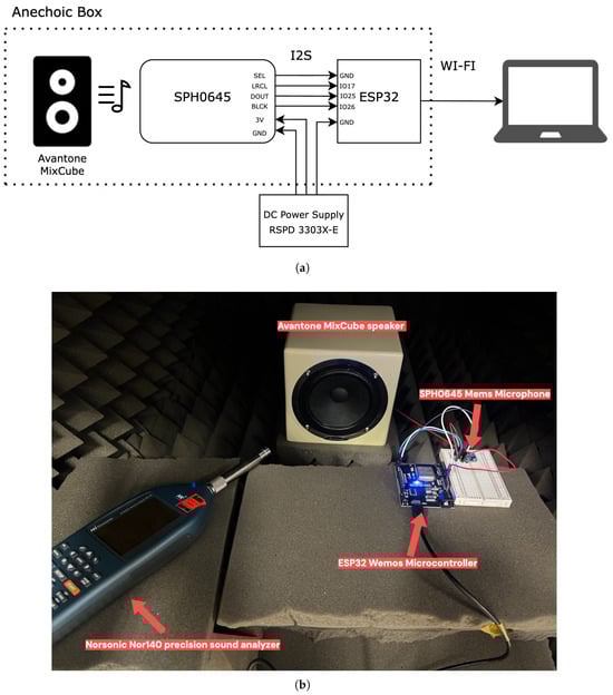
Figure 2.
(a) Schematic diagram of the experimental setup showing the SPH0645 MEMS microphone, ESP32 Wemos microcontroller, DC power supply, and Avantone MixCube speaker. (b) Actual setup in the acoustic chamber with the MixCube speaker, MEMS microphone, ESP32 microcontroller, and Norsonic Nor140 sound analyzer used for SPL calibration.
In all tests, the microphone was positioned 10 cm from the speaker inside an anechoic box to reduce sound reflections and external noise. An anechoic box is a sound-isolated enclosure used to create a quiet and controlled space for audio testing.
All audio was recorded at a sampling rate of 48 kHz with 32-bit resolution. The ESP32 sent the data over Wi-Fi to the host computer using the UDP protocol, which allows fast transmission but does not guarantee packet delivery or order. On the computer, the data was saved in both .csv and .wav formats. Each recording session used a buffer size of 1024 samples, which helped to improve transmission efficiency by reducing the number of packets sent over the network. Prior to data collection, we validated our ESP32 data acquisition code using a LabNation SmartScope logic analyzer (LabNation, Antwerp, Belgium). The logic analyzer results and the data collected from the ESP32 were matching, confirming that the I2S transmission was functioning as expected.
3.2. Sensor Faults
Depending on the type of sensor and the use case, various kinds of faults can arise. In this paper, five different faults: bias, drift, stuck, spike, and clipping, are addressed. Example plots of these faults are shown in Figure 3. Below is a description of some of the most common sensor faults.
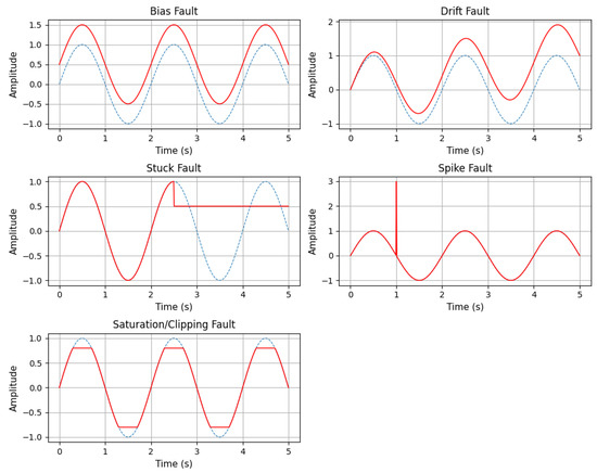
Figure 3.
Types of sensor faults addressed in this study. Each subplot shows how a specific fault, such as bias, drift, stuck, spike, saturation/clipping, affects the sensor signal compared to the normal signal over time. In the plots, the blue dashed line represents the normal signal, while the red line represents the faulty signal.
Mathematically, under ideal conditions without noise, a normal sensor can be represented at time t as Equation (1):
3.2.1. Bias/Offset Fault
Bias faults occur when a sensor’s output consistently deviates from the true value by a fixed amount, often due to calibration issues. The constant bias value b represents this fixed deviation, as shown in Equation (2).
3.2.2. Drift Fault
Drift is a fault where the sensor’s output linearly increases or decreases over time at a constant rate [11]. This can be caused by factors such as aging, temperature fluctuations, or physical damage. The drift rate, denoted as d, represents the change per unit time. The mathematical model for this fault is shown in Equation (3):
3.2.3. Stuck Fault
A stuck fault occurs when a sensor becomes unresponsive and fixed in a certain state, preventing accurate readings. It can be caused by hardware malfunctions or communication problems. This type of fault is represented by the constant value c, as shown in Equation (4).
3.2.4. Spike Fault
A spike fault is a sudden, large change in the sensor data value over a very short time period, deviating from the normal trend [25]. This fault can occur due to a short circuit, an insufficient power supply, or a loose wire connection. When the power supplied to the sensor drops below the minimum required threshold, the sensor may fail to operate correctly, leading to signal spikes. The corresponding mathematical expression is provided in Equation (5), where s represents the spike amplitude, and represents the spike time.
3.2.5. Saturation/Clipping Fault
Saturation occurs when the sensor can no longer react to additional input changes after reaching its maximum or minimum output limit. This may occur as a result of severe operating conditions or restrictions on the sensor’s range. This fault type is mathematically expressed in Equation (6), where represents the upper limit of the sensor output, and represents the lower limit of the sensor output.
3.3. Data Acquisition
Data acquisition in this study focused on collecting both clean and faulty audio signals from a MEMS microphone under various operating conditions. The process began with chirp-based fault characterization to examine how specific faults, such as undervoltage and acoustic overload, impact the microphone’s behavior. Based on these results, real environmental sounds were recorded, and faults were introduced through controlled voltage variations and exposure to loud sound pressure levels. Additionally, synthetic fault injection was applied to clean recordings in order to increase the size and diversity of the dataset.
3.3.1. Chirp-Based Fault Characterization
We used a chirp signal to characterize the behavior of the SPH0645 MEMS microphones under fault conditions and to analyze how the effects of faults vary with frequency, since a chirp signal contains a continuous range of frequencies. This allows us to observe how a fault affects the microphone’s response at different frequency levels across the spectrum. In this study, we used a linear chirp signal because it provides a uniform frequency sweep, making it easier to observe and compare the microphone’s behavior consistently across the entire frequency spectrum. The variables used in the chirp formula are as follows: represents the frequency at time t, is the starting frequency of the chirp, is the ending frequency, T is the total duration of the chirp, and t is the specific time at which the frequency is calculated. The formula of the linear chirp is given in Equation (7):
The signal was generated using Python 3.10.14 at a sample rate of 48 kHz, sweeping steadily from 100 Hz to 20,000 Hz over 5 s. This frequency range was chosen because the microphone’s datasheet shows it is within the valid and relatively flat response range. Two types of controlled tests were conducted on the microphone using the chirp signal, as explained below.
3.3.2. Acoustic Overload Test
To evaluate microphone performance under high sound pressure levels (SPL), chirp signals were played through an Avantone MixCube speaker (Avantone Pro, New York, NY, USA). A 1 kHz sine wave was used to measure the maximum SPL, which reached 129.4 dB. The test was conducted by reducing the SPL in 2 dB steps down to 91.4 dB. Each reduction was converted to a linear scale factor using:
This allowed for accurate scaling of the chirp amplitude. The lower limit of 91.4 dB was chosen to stay below the microphone’s total harmonic distortion threshold. Additionally, a Yamaha MSP5 speaker (Yamaha Corp., Hamamatsu, Japan) was used for cross-validation to ensure observed effects were due to the microphone, not the speaker.
3.3.3. Undervoltage Test
To evaluate how the microphone behaves under low-voltage conditions, its supply voltage was gradually decreased from 3.3 V to 1.5 V using a programmable DC power supply while playing a chirp signal at 90 dB SPL. Since the SPH0645’s minimum operating voltage is 1.62 V, the test began slightly below this value to observe power-related instability. Moreover, this SPL was chosen as it stays below the distortion threshold of the SPH0645 microphone, ensuring faults are due to power instability, not acoustic distortion.
Voltage was varied in different step sizes: from 1.5 V to 1.6 V and from 1.7 V to 3.3 V using 0.10 V steps, and between 1.6 V and 1.7 V using finer 0.05 V steps to capture the microphone’s response near its critical range.
3.3.4. Analysis of Chirp-Based Tests
Analyzing the chirp-based tests was essential to understanding how the microphone behaves under undervoltage and acoustic overload. Instead of introducing artificial faults without a basis, we used real behavior patterns observed during testing to inject realistic faults into clean datasets.
As shown in Figure 4, the microphone operated normally between 91.4 dB and 119.4 dB SPL. Clipping began at 121.4 dB and increased up to 129.4 dB, primarily affecting lower frequencies (100 Hz to 3 kHz). So, the reason for these lower frequencies being affected could be that the microphone is more sensitive to overload, especially at lower frequencies. This might be related to the physical characteristics of the microphone, which is more responsive to low-frequency pressure changes.
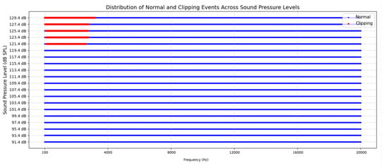
Figure 4.
Distribution of clipping and non-clipping segments across different sound pressure levels (SPLs) and frequencies. Red dots indicate segments where clipping was detected, while blue dots represent normal (non-clipping) segments.
Figure 5 shows the spectrogram results of the undervoltage test. When the voltage was between 1.50 V and 1.65 V, the microphone did not produce any output. Between 1.655 V and 1.700 V, random spikes appeared, but the chirp signal was not visible, meaning the microphone was unstable. At 1.71 V and 1.72 V, the chirp signal appeared with spikes. The 1.71 V level was chosen for injecting spike faults, since it showed partial output with clear signs of failure. From 1.73 V to 3.30 V, the microphone worked normally. However, some recordings still showed a small amount of noise, which could be due to minor electrical interference, environmental noise, or wireless data transmission.
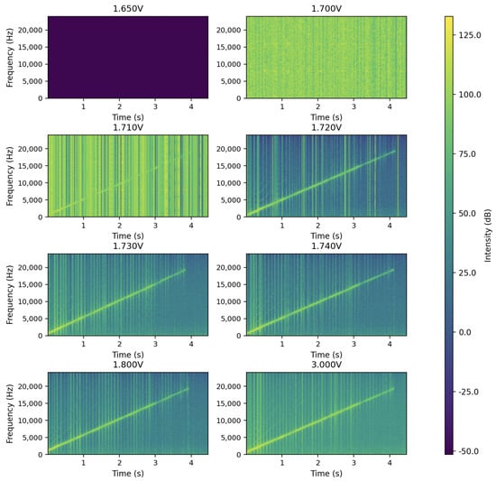
Figure 5.
Spectrograms of chirp signals recorded at different voltage levels.
3.3.5. Fault Data Collection
After the chirp-based tests, we collected fault and normal data using real sounds. Audio clips were taken from the BDLib2 Environmental Sound Dataset, which includes 10-s samples from 10 sound categories like airplanes, alarms, rain, and thunder [26,27].
These sounds were played through a speaker while applying the voltage and SPL levels found during earlier tests (Table 2). In order to provide a complete dataset, we also recorded the same audio clips without any faults under standard operating conditions. This helped us simulate realistic faults in real environments and use the data to test the model’s ability to detect sensor faults.
Table 2.
Overview of voltage and SPL conditions used for real fault injection and clean data collection. Each fault type was induced by applying specific voltage and SPL, based on prior chirp signal analysis. These conditions were used to simulate realistic sensor behaviors in the dataset.
3.4. Synthetic Fault Injection
To increase the dataset size, synthetic faults were injected into clean audio recordings from the BDLib2 dataset. Specifically, bias and drift faults were added to simulate sensor issues that are hard to reproduce physically.
These faults were generated using custom Python scripts adapted from publicly available code on GitHub [28]. For drift injection, the fault was applied over the entire duration of the signal. The drift increment was calculated by dividing the maximum absolute amplitude by twice the total number of samples. This increment was then linearly added to each sample in the signal, resulting in a gradual increase or decrease over time. The drift direction was randomly selected. This method effectively simulates real-world drift behavior typically caused by long-term factors such as sensor aging or environmental influence. Algorithm 1 illustrates the process of drift fault injection.
| Algorithm 1 Drift Fault Injection |
Input: Clean signal S of length N Output: Drifted signal
|
For bias fault injection, a constant value was added to each biased part of the signal to simulate a shift in sensor output. Each biased part was selected by randomly choosing a start index and duration within the signal. The bias value was calculated by taking the highest absolute value in that part of the signal and multiplying it by a random percentage between 20% and 30%. The bias could be either positive or negative and remained constant throughout the selected portion. The duration of each biased part ranged between 0.1 s and 1.0 s, depending on the total length and sampling rate of the signal. This duration range was chosen to simulate short-term bias faults that are long enough to be detected but not so long that they dominate the entire signal. The pseudo code for bias fault injection is given in Algorithm 2.
| Algorithm 2 Bias Fault Injection |
Input: Clean Signal S of length N, number of segments K, duration range Output: Biased signal
|
These synthetic faults were injected directly into real normal data to create new fault samples. These synthetic faults helped expand the dataset and support the model in learning to detect more types of sensor failures.
3.5. Dataset Preprocessing
Before training the classification models, several preprocessing steps were applied to ensure consistency in data formatting, improve signal quality, and structure the input for classifiers. Short silent segments at the beginning and end of some recordings were removed due to Wi-Fi transmission delays or data buffering. To prepare the audio signals for classification, 1-s and 2-s sliding windows with 50% overlap were used. The overlapping means each new window starts in the middle of the previous one, helping to detect changes in the signal and accurately identify fault beginnings and endings.
Visualization of the 1 s sliding window segmentation is shown in Figure 6. A similar approach was applied for the 2 s window. Since the audio was trimmed to remove silence, the remaining signal had a length of X seconds, depending on the original recording. The trimmed signal was then divided into N windows, with each window serving as one input for the AI model. Each window was labeled based on the presence of faults, with the entire window assigned the fault label if any part of it contained a fault. Maximum-Absolute (Max-Abs) normalization was applied to each sliding window to improve model training and ensure consistency across input samples. Each sample was divided by the maximum absolute value within the window, bringing all values into a range between −1 and 1 while preserving the signal shape.
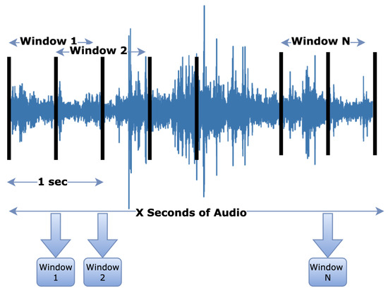
Figure 6.
Visualization of the 1 s sliding window segmentation to extract the N windows from the X seconds of the audio file used for training.
3.6. Fault Classification
We employed several classification models that are frequently used in the literature. This analysis focuses on lightweight models designed for real-time classification tasks. These models have demonstrated strong performance in fault classification tasks. Specifically, we used a 1D CNN, Random Forest, Decision Tree, Extremely Randomized Trees, XGBoost, and an MLP.
Since traditional ML models cannot operate directly on raw time-series data, feature extraction is necessary. However, manual feature extraction requires significant domain expertise and time. In real-time systems, this added processing can slow down performance and cause delays in response time. To address this, we used an automatic feature extraction approach using a CNN. The CNN extracts features directly from the raw input signals and feeds them to the ML classifiers. This hybrid strategy is also widely used and validated in related works [1,20].
Additionally, we used a standalone 1D CNN as a deep learning baseline, which performs both feature extraction and classification in an end-to-end manner. 1D CNNs are widely used in classification tasks and have shown good performance with time-series and audio data, making them a suitable choice for our fault classification system [29,30].
Although more advanced deep learning models might give better results, we decided to use simpler models because of hardware and computational limits. Deep learning models often need a lot of processing power, and they can consume a lot of energy. This is a big issue when using them in real-world systems [4]. For this reason, we chose lightweight models that give good performance but still work well on resource-constrained devices. All selected models were compared systematically during the final evaluation phase.
Training and Evaluation Setup
All evaluations were done locally on a MacBook Air with an Apple M2 chip, 16 GB of RAM, and a 256 GB SSD, running macOS Sequoia. The software environment used Python 3.13. Deep learning models were built using the PyTorch 2.7.0 library, and classical ML models were developed and tested with Scikit-learn 1.6.1 library.
The dataset was split into three parts using a stratified approach with 70% for training, 20% for validation, and 10% for testing. Class distribution was preserved through stratified sampling within each class, ensuring that all subsets reflected the overall balance of fault types. This was particularly important when working with imbalanced datasets.
We used two CNN-based architectures. The first one is an end-to-end model called CNNClassifier. The second one is a feature extraction model called CNNFeatureExtractor (CNNFE). We chose these names to clearly show their different purposes in the rest of the paper.
The training of the CNNClassifier was conducted using the Adam optimizer, which adapts the learning rate for each parameter, with an initial learning rate of 0.001. A batch size of 4 was used, meaning the model updated its weights after every 4 samples. The training ran for up to 100 epochs, where one epoch represents a full pass through the training data. To handle the imbalance between classes, we used weighted cross-entropy loss. Early stopping was also used with a patience of 10 epochs, which stopped training if validation performance did not improve after 10 consecutive epochs. These training parameters were selected based on commonly used values in the literature and are suitable for lightweight CNN models. A relatively small batch size was chosen due to the memory limitations of the evaluation hardware. The architecture and hyperparameters for the CNN-based models were derived from previous studies [31,32], which focused on resource-constrained devices, as summarized in Table 3.
Table 3.
Architecture and parameter summary of the CNNClassifier with a 1 s window size and 6-class output. k denotes the kernel size, and p denotes the padding used in convolutional layers.
Table 3 presents the architecture of the CNNClassifier, which is designed for audio input with a 1-s window size. For six classes, the model has a total of 18,054 trainable parameters, while for four classes, it has 4004 trainable parameters. For 2-s windows, the parameter count remains unchanged; only the intermediate output shapes vary.
The same architecture and parameters used in CNNClassifier were also applied to CNNFeatureExtractor, except that the final classification layers were removed, as shown in Table 4. For feature extraction for ML models, we used an untrained CNN, as existing research has shown that even without pretraining, randomly initialized CNNs can still learn meaningful representations from data [33,34]. They still apply filters across the signal in a way that respects the temporal structure. This creates feature representations that, while random, still preserve meaningful temporal relationships. Since untrained CNNs do not require backpropagation or weight updates, they are computationally less intensive, making them suitable for scenarios with limited resources.
Table 4.
Architecture and parameter summary of the CNNFeatureExtractor with a 1 s window size. The model outputs a 32-dimensional latent feature vector. k denotes the kernel size, and p denotes the padding used in convolutional layers.
The hyperparameters for the ML models were also derived from existing research. More details can be found in these papers [5,6,35]. The specific hyperparameter settings for each model are summarized in Table 5.
Table 5.
Hyperparameters used for each classifier model.
3.7. Evaluation Metrics
It is essential to evaluate the model with unseen data to assess its performance on data it has not encountered during training. We used accuracy, F1 score, inference time, and model size as evaluation metrics, which are particularly relevant for real-time applications and embedded devices, helping determine the best model for deployment in terms of reliability, size, and latency [36].
3.7.1. Accuracy
Accuracy is one of the metrics used to evaluate model performance. Accuracy shows how correct the classifier is by comparing the number of true predictions to the total number of predictions. As shown in Equation (9), it is computed as the sum of true positives and true negatives, divided by the total number of instances. Here, represents the number of true positives, is the number of true negatives, represents the number of false positives, and is the number of false negatives.
3.7.2. F1 Score
The F1 score is a metric that combines precision and recall using the harmonic mean. Precision measures how accurate the predicted positive results are, as shown in Equation (10), while recall shows how many of the actual positive samples are correctly classified as positive, as seen in Equation (11). These metrics are defined as follows:
F1 score is calculated using Equation (12):
The F1 score is particularly useful in scenarios involving imbalanced datasets, as it reflects both the model’s ability to correctly identify positive samples and its accuracy in avoiding false alarms.
3.7.3. Inference Time
Inference time is the amount of time a model needs to process one input sample and deliver a prediction. In our work, we calculated inference time by running each model on all test samples and then computing the mean and standard deviation of the results.
3.7.4. Model Size
Model size refers to the storage footprint of the trained model in kilobytes (kB). It is an important factor when selecting models for deployment on resource-constrained devices, as such devices typically have limited storage capacity.
4. Results
4.1. Experiment 1: Evaluation of Classifiers with Varying Window Sizes on Real Fault Data
In the first experiment, we evaluated different classifier models using real sensor fault data with two different window sizes: 1 s and 2 s. Table 6 shows the distribution of windows per class in the training, validation, and test sets for both 1 s and 2 s input windows.
Table 6.
Number of windows per class for training (70%), validation (20%), and test (10%) sets using (a) 1 s and (b) 2 s input windows. Each 1 s window contains 48,000 audio samples; each 2 s window contains 96,000 audio samples of real fault data.
As shown in Figure 7, all models performed very well, with high accuracy and F1-scores for most fault types. For the stuck fault, every model achieved 100% accuracy and F1-score. It shows that it was easy to detect when the sensor completely stopped working. This result is expected, as the values remain stuck at zero, making the fault easy to classify. However, according to the results, classifying the clipping fault was more difficult across all models. When we increased the window size to 2 s, we observed that the performance slightly increased for all fault types. For example, the CNNClassifier’s average accuracy increased from 97.13% to 98.18%, and its F1-score improved from 94.92% to 97.17%. Average accuracy and F1-score improved across nearly all configurations, as shown more clearly in Figure 8. This indicates that the additional temporal context helps in identifying fault patterns like clipping. Additionally, the detection of the stuck fault maintained perfect accuracy and F1-score across all models, regardless of the window size, thanks to its unchanging nature.
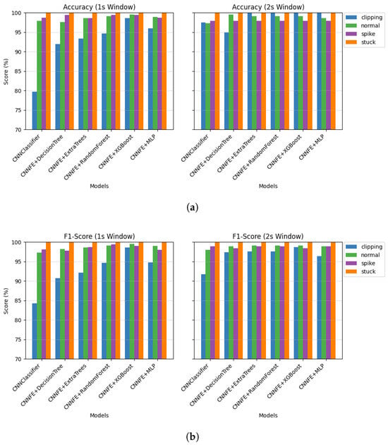
Figure 7.
Performance comparison of classifiers on real fault data using different window sizes: (a) Accuracy and F1-score for each fault type (clipping, normal, spike, stuck) using a 1 s sliding window. (b) Accuracy and F1-score using a 2 s sliding window. Models include a standalone CNN classifier and CNN-based feature extractors combined with classical ML classifiers (Decision Tree, Extra Trees, Random Forest, XGBoost, and MLP). Each bar represents the per-class metric score (%), illustrating how both window size and model architecture affect classification performance across different fault types.
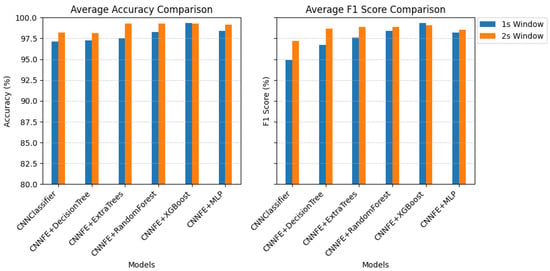
Figure 8.
Average accuracy and F1-score comparison across models using 1 s and 2 s windows of real fault data.
Figure 8 compares the average scores for all models using both window sizes. It shows that most models performed better with the 2 s window input.
Figure 9 compares the model sizes and shows that some models became smaller when using 2 s input windows. For example, the CNNFE+ExtraTrees model dropped from 2119.73 kB with 1 s inputs to 805.92 kB with 2 s inputs. Although the same architectures and hyperparameters were used, model sizes changed due to fewer training samples. This led to smaller models like Decision Trees, ExtraTrees, Random Forest, and XGBoost, which build simpler trees with fewer splits when trained on less data. In contrast, CNNClassifier and MLP have fixed architectures, so their sizes remain unchanged.
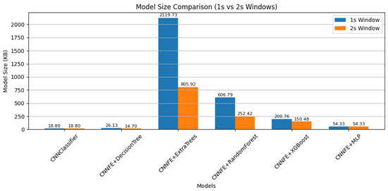
Figure 9.
Model size comparison (in KB) across classifiers using 1 s and 2 s windows of real fault data.
Inference time is shown in Figure 10. All models took slightly longer to make predictions with 2 s inputs. For example, the CNNClassifier’s inference time increased from 3.05 ± 0.48 ms to 5.30 ± 0.69 ms, corresponding to a 73.80% rise. Similarly, CNNFE+MLP went from 2.23 ± 1.46 ms to 4.17 ± 0.95 ms, an 87.00% increase. This is expected because 2 s windows contain 96,000 samples compared to 48,000 in 1 s windows. The larger input size requires more computation during both feature extraction and classification. Therefore, even though the model architecture remains the same, longer inputs result in increased inference time.
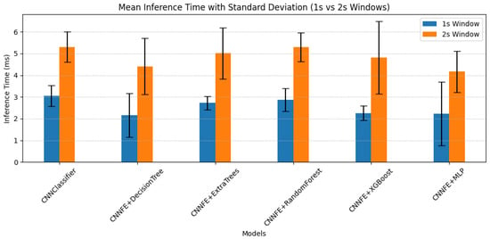
Figure 10.
Mean inference time with standard deviation for each model using 1 s and 2 s windows.
4.2. Experiment 2: Evaluation of Classifiers with Varying Window Sizes on Combined Real and Synthetic Fault Data
In the second experiment, we evaluated the performance of the classification models on a combined dataset that includes both real and synthetically injected faults. The two synthetic fault types we added were bias and drift. This helped us to see how the window length affects model performance when using both real and synthetic data. Table 7 shows how each fault class is divided into training, validation, and test sets based on the number of windows.
Table 7.
Number of windows per class for training (70%), validation (20%), and test (10%) sets using (a) 1 s and (b) 2 s input windows. Each 1 s window contains 48,000 audio samples; each 2 s window contains 96,000 audio samples.
As shown in Figure 11, the models overall performed better when using the 2 s window. This matches what we saw in the first experiment and shows that a longer window helps the models detect and understand the faults more accurately. CNNFE+RandomForest, CNNFE+ExtraTrees and CNNFE+XGBoost achieved over 98% accuracy and over 94% F1-score for bias and spike in both window sizes. Stuck faults reached 100% accuracy in all models, indicating their clear and distinct fault signature.
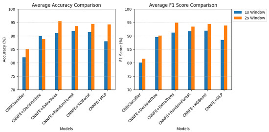
Figure 11.
Average accuracy and F1-score comparison across models using 1 s and 2 s windows of real and synthetic fault data.
The performance of the CNN Classifier for detecting the ”normal” class was quite low compared to other classes, as can be seen in Figure 12. In the 1 s window results, the model reached only 47.74% accuracy and 60.97% F1-score for the normal class. With the 2 s window, the performance dropped even more, to 45.50% accuracy and 59.51% F1-score. These are the lowest results among all classes. One possible reason is that drift faults were sometimes mistaken for normal behavior. Since drift changes slowly over time, it can look similar to normal signals at first. This may have caused the model to confuse the two, leading to poor performance for the normal class. In contrast, the models that used CNN feature extraction followed by ML classifiers (such as Decision Tree, Extra Trees, Random Forest, XGBoost, and MLP) showed much better results for the normal class. Most of these models achieved around 90% or higher accuracy and F1-score for normal classification with both 1 s and 2 s windows. This shows that using feature extraction helps the models better separate normal signals from faults, including difficult cases like drift.
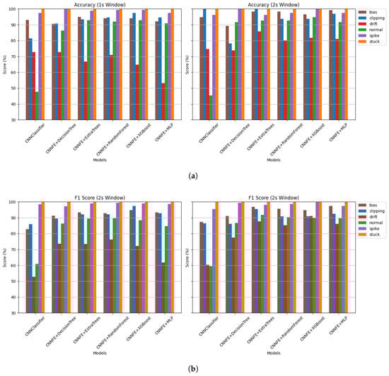
Figure 12.
Performance comparison of classifiers on real and synthetic fault data using different window sizes. (a) Accuracy and F1-score for each fault type (clipping, normal, spike, stuck) using a 1 s sliding window. (b) Accuracy and F1-score using a 2 s sliding window. Models include a standalone CNN classifier and CNN-based feature extractors combined with classical ML classifiers (Decision Tree, Extra Trees, Random Forest, XGBoost, and MLP). Each bar represents the per-class metric score (%), illustrating how both window size and model architecture affect classification performance across different fault types.
Model sizes are shown in Figure 13. Among all models, the CNNClassifier had the smallest size (only 19.30 kB), making it suitable for highly resource-constrained devices. However, this comes at the cost of significantly lower accuracy and F1-score. In contrast, the CNNFE+ExtraTrees model was the largest, with a size of 14,989.96 kB for the 1 s window and 5361.24 kB for the 2 s window. Although this model performed well in terms of classification, its large memory footprint may limit its use in resource-limited systems. Also, as observed in the first experiment, using a 2 s window reduced the model size for all tree-based models. This is mainly because the number of training windows decreased, which led to the construction of simpler trees with fewer splits and, consequently, smaller model sizes.
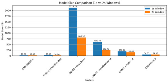
Figure 13.
Model size comparison (in KB) across classifiers using 1 s and 2 s windows of real and synthetic fault data.
Inference times for both window sizes are shown in Figure 14. All models took longer with the 2 s window because the input doubled from 48,000 to 96,000 samples, increasing computation. CNNFE+DecisionTree was the fastest, averaging 2.23 ms for 1 s and 4.07 ms for 2 s windows, which is about an 82.5% increase. CNNFE+ExtraTrees was the slowest, rising from 2.84 ms to 5.45 ms. Although ExtraTrees gave good accuracy, it required significantly higher computation time.
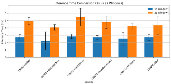
Figure 14.
Mean inference time with standard deviation for each model using 1 s and 2 s windows of real and synthetic fault data.
The comparison between the combined dataset (real + synthetic faults) and the real fault dataset shows that models performed better when trained and tested only on real faults. Accuracy and F1-scores were higher, especially with the 2 s window. For example, CNNFE+ExtraTrees and CNNFE+XGBoost reached about 99% accuracy and F1-score with real faults but dropped to around 95% on the combined dataset. The drop is due to harder faults like drift, which change slowly and look like normal signals. Stuck and spike faults were classified well in all cases. Model size and inference time stayed similar. Overall, models using CNN feature extraction plus classical classifiers outperformed the CNNClassifier, and real fault data gave more accurate results because synthetic faults made classification harder.
4.3. Experiment 3: Performance Evaluation Across Audio Categories
The experimental results in this section show a detailed analysis of how well different models can classify faults in various environmental sound categories using different window sizes. As in the previous experiments, a CNN Feature Extractor was used to get important features from the audio signals. In the figures, only the names of the ML models are written, but all of them used the same CNN features. In this experiment, as in the previous experiments, we used CNN combined with machine learning models such as Decision Tree, Extra Trees, Multi-Layer Perceptron, and XGBoost, but the CNNClassifier was not used. There are two main reasons for this. First, in the earlier experiments, the CNNClassifier gave lower accuracy compared to other models. Second, running CNNClassifier requires higher computational resources, especially during evaluation. Since all evaluations were conducted on a device with limited computing capacity, the use of the CNNClassifier was not efficient. Because of this, we chose to use lighter ML models that are faster and easier to run. Table 8 shows the number of samples per fault type for each sound category, using 1 s and 2 s windows, respectively. In both datasets, each sound category (such as airplane, alarms, applause, birds, etc.) includes six types of signals: normal, drift, stuck, spike, bias, and clipping.
Table 8.
Number of samples per fault type and sound category for (a) 1 s and (b) 2 s window datasets. Each cell shows how many windows belong to a specific fault type (normal, drift, stuck, spike, bias, and clipping) for each environmental sound category. The total number of samples per category is shown in the last row.
Figure 15 shows the classification accuracy and F1 score of the five ML models for each sound category using 1 s and 2 s windows. They achieved reasonably good accuracy overall; however, the MLP model performed noticeably worse in some cases. For example, while most models achieved around 80% accuracy on the “rain” category, the MLP model only reached 68.25%. Similarly, for the “rivers” category, where other models performed around 87%, MLP achieved only 79.84%. This lower performance could be due to the simpler structure of the MLP model, which may not capture complex temporal or frequency patterns as effectively as other tree-based models.
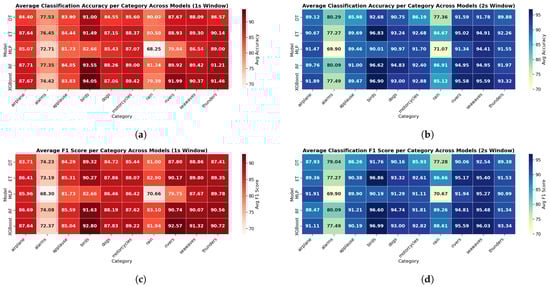
Figure 15.
Average classification accuracy and F1-score per environmental sound category across different models using 1 s and 2 s sliding windows: (a) Average classification accuracy for the 1 s window. (b) Average classification accuracy for the 2 s window. (c) Average F1-score for the 1 s window. (d) Average F1-score for the 2 s window. The results illustrate the classification performance of each model (Decision Tree, Extra Trees, MLP, Random Forest, XGBoost) across various sound categories in 1-s and 2-s window sizes.
Moreover, all models showed lower performance in the “alarms” and “rain” categories compared to others. For example, the MLP model achieved only 68.25% accuracy on “rain” and 72.71% on “alarms”. One possible reason is that the audio signals in “alarms” and “rain” can be more complex and change more quickly. When the window size was increased to 2 s, the accuracy of all models improved across most categories. However, even with this improvement, the accuracy for “alarms” and “rain” still remained lower than for other categories. This suggests that although using longer input windows helps by providing more temporal context, it does not fully overcome the difficulty of detecting faults like alarms and rain. The MLP model also benefited from the longer input window and showed noticeable improvements in several categories. One clear example is the “rivers” category, where its accuracy increased from 79.84% to 91.34%.
Figure 16 analyzes the model performance based on fault types and how their detection accuracy and F1 score change across different sound categories. It shows that for 1 s windows, “stuck” faults are detected with 100% accuracy in all categories, and “spike” faults are also easy to detect, with accuracy above 93.80%. These faults create clear patterns in the signal, which makes them easier for the models to recognize. “Bias” faults also perform well, with accuracy usually above 85%, as they cause a consistent shift in the signal that is easier to learn. In contrast, “clipping” and “drift” faults are more difficult to detect, and their accuracy varies depending on the sound category. For instance, in the “rain” category, clipping accuracy drops to 36.67%, likely due to the small number of available clipping samples. Drift faults also show lower accuracy, ranging from 40.87% to 73.92% across categories. However, it is important to note that clipping faults perform much better in other categories. For example, in “applause” and “birds,” where the number of clipping samples is higher and the fault pattern may be more distinguishable, accuracy reaches much higher levels.
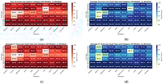
Figure 16.
Average classification accuracy and F1-score per fault type and environmental sound category across all models using 1 s and 2 s sliding windows: (a) Average classification accuracy for 1 s window. (b) Average classification accuracy for 2 s window. (c) Average F1-score for 1 s window. (d) Average F1-score for 2 s window. The results illustrate the classification performance across different fault types (normal, drift, clipping, bias, spike, stuck) and sound categories in 1 s and 2 s window sizes.
In the 2 s window, accuracy and F1 score improved for all fault types. For example, clipping accuracy in “rain” increases from 36.67% to 46.67%, and drift accuracy improves by 5–10% in most categories. In categories like “birds,” “dogs,” and “motorcycles” clipping accuracy reached nearly 100%. Drift F1-score in “alarms” improves from 44.90% to 56.03%, and clipping F1 in “rain” improves from 44.57% to 50.73%. These results show that while longer windows help, they do not fully solve the problem. Faults that develop slowly over time, like drift, or that have very few samples, like clipping, remain challenging.
4.4. Discussion
Experiment 1 showed that using a 2 s window improves model performance across all classifiers by providing more temporal context, especially for detecting spike and stuck faults. Although this increased inference time slightly (e.g., CNNFE+MLP latency rose from 2.23 ms to 4.17 ms), the improvement in accuracy justified the trade-off. The increase in inference time is expected, as longer input windows contain more data, requiring more processing during feature extraction and classification. Tree-based models (Decision Trees, Extra Trees, Random Forest, and XGBoost) had reduced model sizes due to fewer training samples with the larger window. On the other hand, models like CNNClassifier and MLP have a fixed structure and number of parameters, so their model sizes do not change based on the amount of training data.
CNNFE+XGBoost and CNNFE+MLP emerged as strong candidates due to their high accuracy, low inference time, and small model size, making them suitable for embedded deployment. CNNFE+XGBoost achieved up to 99.25% accuracy and 99.07% F1 with only 150.48 kB, while CNNFE+MLP achieved 98.55% F1 with 54.33 kB.
In Experiment 2, adding synthetic faults (drift, bias) made classification harder, especially for subtle faults like drift. Still, the 2 s window improved results. CNNFE+XGBoost achieved a 94.47% F1-score with a model size of only 309.90 kB. CNNFE+ExtraTrees achieved a 95.03% F1-score with a model size of 5361.24 kB. CNNFE+MLP reached a 93.85% F1-score, confirming the robustness of these models even under more complex fault conditions.
Experiment 3 revealed that sound category impacts model performance. Categories like “alarms” and “rain” were more challenging, especially for clipping and drift faults. Clipping detection in “rain” reached only 36.67% accuracy with a 1 s window. Drift detection varied significantly across categories, even when the sample size was constant, suggesting a strong influence of signal characteristics.
Overall, Extra Trees and XGBoost performed especially well. The reason can be that both models handle high-dimensional CNN features very efficiently and can focus on the most important patterns in the extracted representation. Extra trees’ primary parameters are the number of trees, the number of random features taken into account at each node, and the minimum number of samples required for splitting a node. This model does not require a lot of adjustments and naturally balances different types of errors, such as bias and variance. This balance helps the model produce consistent and accurate predictions [5]. XGBoost uses boosted trees that correct errors step by step, allowing it to capture subtle differences in the features. These strengths make both models highly effective at identifying normal behavior in the extracted feature space.
However, CNNFE+XGBoost demonstrated the most consistent and reliable performance across fault types and sound environments, while balancing memory and latency constraints. Despite the promising results, no hyperparameter tuning was applied in this study, and further optimization could enhance model performance and efficiency even more.
5. Conclusions
This study investigated the use of ML for classifying faults in MEMS microphone sensors, focusing on lightweight models for resource-constrained devices. A dataset was developed with both real-world faults (clipping, spike, stuck) and synthetic faults (drift, bias). Various models, including CNNs and traditional ML models like Random Forest, Decision Tree, Extra Trees, XGBoost, and MLP, were tested. A hybrid approach using CNNs as feature extractors achieved strong performance without manual feature engineering for traditional ML models.
The evaluation showed that 2 s windows improved accuracy and F1-scores, though they slightly increased inference time and reduced model sizes, particularly for tree-based models. We also examined how the models performed across various sound categories and observed that different sound categories had a noticeable impact on fault classification accuracy, with some conditions making classification more difficult. The results demonstrate that ML-based fault classification offers reliable performance, with CNNFE+XGBoost being the most suitable for resource-constrained devices. Future research could focus on hyperparameter tuning, real-time testing on embedded devices to assess latency and classification reliability, and expanding the dataset to improve model robustness in real-world conditions.
Author Contributions
Conceptualization, B.T. and B.d.S.; methodology, B.T.; software, B.T.; validation, B.T.; investigation, B.T.; resources, B.T. and B.d.S.; data curation, B.T. and J.V.V.; writing—review and editing, B.T. and B.d.S.; visualization, B.T.; supervision, B.d.S. and J.V.V.; project administration, B.d.S. All authors have read and agreed to the published version of the manuscript.
Funding
This research received no external funding.
Data Availability Statement
The dataset is available in Zenodo 10.5281/zenodo.17641389 and the code is maintained in https://gitlab.com/etrovub/embedded-systems/publications/lightweight-AI-for-sensor-fault-monitoring, all accessed on 26 October 2025.
Conflicts of Interest
The authors declare no conflicts of interest.
References
- Seba, A.M.; Gemeda, K.A.; Ramulu, P.J. Prediction and classification of IoT sensor faults using hybrid deep learning model. Discov. Appl. Sci. 2024, 6, 9. [Google Scholar] [CrossRef]
- Anik, M.T.H.; Fadaeinia, B.; Moradi, A.; Karimi, N. On the impact of aging on power analysis attacks targeting power-equalized cryptographic circuits. In Proceedings of the 26th Asia and South Pacific Design Automation Conference, Tokyo Japan, 18–21 January 2021; pp. 414–420. [Google Scholar]
- Agarwal, A.; Sinha, A.; Das, D. FauDigPro: A Machine Learning based Fault Diagnosis and Prognosis System for Electrocardiogram Sensors. In Proceedings of the 2022 International Conference on Maintenance and Intelligent Asset Management (ICMIAM), Anand, India, 12–15 December 2022; pp. 1–6. [Google Scholar]
- Hasan, M.N.; Jan, S.U.; Koo, I. Sensor Fault Detection and Classification Using Multi-Step-Ahead Prediction with an Long Short-Term Memory (LSTM) Autoencoder. Appl. Sci. 2024, 14, 7717. [Google Scholar] [CrossRef]
- Saeed, U.; Lee, Y.D.; Jan, S.U.; Koo, I. CAFD: Context-aware fault diagnostic scheme towards sensor faults utilizing machine learning. Sensors 2021, 21, 617. [Google Scholar] [CrossRef]
- Saeed, U.; Jan, S.U.; Lee, Y.D.; Koo, I. Fault diagnosis based on extremely randomized trees in wireless sensor networks. Reliab. Eng. Syst. Saf. 2021, 205, 107284. [Google Scholar] [CrossRef]
- Min, H.; Fang, Y.; Wu, X.; Lei, X.; Chen, S.; Teixeira, R.; Zhu, B.; Zhao, X.; Xu, Z. A fault diagnosis framework for autonomous vehicles with sensor self-diagnosis. Expert Syst. Appl. 2023, 224, 120002. [Google Scholar] [CrossRef]
- Zidi, S.; Moulahi, T.; Alaya, B. Fault detection in wireless sensor networks through SVM classifier. IEEE Sensors J. 2017, 18, 340–347. [Google Scholar] [CrossRef]
- Sinha, A.; Das, D. XAI-LCS: Explainable AI-Based Fault Diagnosis of Low-Cost Sensors. IEEE Sensors Lett. 2023, 7, 1–4. [Google Scholar] [CrossRef]
- Novak, A.; Honzík, P. Measurement of nonlinear distortion of MEMS microphones. Appl. Acoust. 2021, 175, 107802. [Google Scholar] [CrossRef]
- Saeed, U.; Jan, S.U.; Lee, Y.D.; Koo, I. Machine learning-based real-time sensor drift fault detection using Raspberry PI. In Proceedings of the 2020 International Conference on Electronics, Information, and Communication (ICEIC), Barcelona, Spain, 19–22 January 2020; pp. 1–7. [Google Scholar]
- Suthaharan, S.; Alzahrani, M.; Rajasegarar, S.; Leckie, C.; Palaniswami, M. Labelled data collection for anomaly detection in wireless sensor networks. In Proceedings of the 2010 Sixth International Conference on Intelligent Sensors, Sensor Networks and Information Processing, Brisbane, QLD, Australia, 7–10 December 2010; pp. 269–274. [Google Scholar]
- Biddle, L.; Fallah, S. A Novel Fault Detection, Identification and Prediction Approach for Autonomous Vehicle Controllers Using SVM. Automot. Innov. 2021, 4, 301–314. [Google Scholar] [CrossRef]
- Noshad, Z.; Javaid, N.; Saba, T.; Wadud, Z.; Saleem, M.Q.; Alzahrani, M.E.; Sheta, O.E. Fault detection in wireless sensor networks through the random forest classifier. Sensors 2019, 19, 1568. [Google Scholar] [CrossRef]
- Jan, S.U.; Lee, Y.D.; Shin, J.; Koo, I. Sensor fault classification based on support vector machine and statistical time-domain features. IEEE Access 2017, 5, 8682–8690. [Google Scholar] [CrossRef]
- Warriach, E.U.; Tei, K. Fault detection in wireless sensor networks: A machine learning approach. In Proceedings of the 2013 IEEE 16th International Conference on Computational Science and Engineering, Sydney, NSW, Australia, 3–5 December 2013; pp. 758–765. [Google Scholar]
- Zhu, M.; Li, J.; Wang, W.; Chen, D. Self-Detection and Self-Diagnosis Methods for Sensors in Intelligent Integrated Sensing System. IEEE Sensors J. 2021, 21, 19247–19254. [Google Scholar] [CrossRef]
- Robinson Luque, C.E. Edge AI for Real-Time Anomaly Classification in Solar Photovoltaic Systems. 2023. Available online: https://scholar.google.com/scholar?hl=es&as_sdt=0%2C5&q=Edge+AI+for+real-time+anomaly+classification+in+solar+photovoltaic+systems&btnG=% (accessed on 26 October 2025).
- Lin, T.H.; Zhang, X.R.; Chen, C.P.; Chen, J.H.; Chen, H.H. Learning to identify malfunctioning sensors in a large-scale sensor network. IEEE Sensors J. 2021, 22, 2582–2590. [Google Scholar] [CrossRef]
- Sinha, A.; Das, D. An explainable deep learning approach for detection and isolation of sensor and machine faults in predictive maintenance paradigm. Meas. Sci. Technol. 2023, 35, 015122. [Google Scholar] [CrossRef]
- Group, M.D. MIT Computer Science and Artificial Intelligence Laboratory (CSAIL) Sensor Data. 2024. Available online: http://db.csail.mit.edu/labdata/labdata.html (accessed on 28 May 2025).
- De Bruijn, B.; Nguyen, T.A.; Bucur, D.; Tei, K. Benchmark datasets for fault detection and classification in sensor data. In Proceedings of the 5th International Confererence on Sensor Networks, Rome, Italy, 19–21 February 2016; pp. 185–195. Available online: https://research.rug.nl/files/128994363/SENSORNETS_2016_14.pdf (accessed on 26 October 2025).
- Poornima, I.G.A.; Paramasivan, B. Anomaly detection in wireless sensor network using machine learning algorithm. Comput. Commun. 2020, 151, 331–337. [Google Scholar] [CrossRef]
- Azzouz, I.; Boussaid, B.; Zouinkhi, A.; Abdelkrim, M.N. Multi-faults classification in WSN: A deep learning approach. In Proceedings of the 2020 20th International Conference on Sciences and Techniques of Automatic Control and Computer Engineering (STA), Sfax, Tunisia, 20–22 December 2020; pp. 343–348. [Google Scholar]
- Jan, S.U.; Lee, Y.D.; Koo, I.S. A distributed sensor-fault detection and diagnosis framework using machine learning. Inf. Sci. 2021, 547, 777–796. [Google Scholar] [CrossRef]
- Bountourakis, V.; Vrysis, L.; Papanikolaou, G. Machine Learning Algorithms for Environmental Sound Recognition: Towards Soundscape Semantics. In Proceedings of the Audio Mostly 2015 on Interaction With Sound, Thessaloniki, Greece, 7–9 October 2015; pp. 1–7. [Google Scholar]
- Bountourakis, V.; Vrysis, L.; Konstantoudakis, K.; Vryzas, N. An Enhanced Temporal Feature Integration Method for Environmental Sound Recognition. Acoustics 2019, 1, 410–422. [Google Scholar] [CrossRef]
- Chang, E. Sensor Failure Detection. 2023. Available online: https://github.com/ethanchang34/sensor-failure-detection (accessed on 15 May 2025).
- Jana, D.; Patil, J.; Herkal, S.; Nagarajaiah, S.; Duenas-Osorio, L. CNN and Convolutional Autoencoder (CAE) based real-time sensor fault detection, localization, and correction. Mech. Syst. Signal Process. 2022, 169, 108723. [Google Scholar] [CrossRef]
- Vandendriessche, J.; Wouters, N.; da Silva, B.; Lamrini, M.; Chkouri, M.Y.; Touhafi, A. Environmental sound recognition on embedded systems: From FPGAs to TPUs. Electronics 2021, 10, 2622. [Google Scholar] [CrossRef]
- Al-Libawy, H. Efficient implementation of a tiny deep learning classifier based on vibration-related fault detection using limited resources. J. Univ. Babylon Eng. Sci. 2025, 88–105. Available online: https://journalofbabylon.com/index.php/JUBES/article/view/5622?articlesBySimilarityPage=3 (accessed on 26 October 2025).
- Abd Elaziz, M.; Fares, I.A.; Aseeri, A.O. Ckan: Convolutional kolmogorov—Arnold networks model for intrusion detection in IoT environment. IEEE Access 2024, 12, 134837–134851. [Google Scholar] [CrossRef]
- Li, X.; Xi, W.; Lin, J. Randomnet: Clustering time series using untrained deep neural networks. Data Min. Knowl. Discov. 2024, 38, 3473–3502. [Google Scholar] [CrossRef]
- Tong, Z.; Tanaka, G. Reservoir computing with untrained convolutional neural networks for image recognition. In Proceedings of the 2018 24th International Conference on Pattern Recognition (ICPR), Beijing, China, 20–24 August 2018; pp. 1289–1294. [Google Scholar]
- Mazibuco, V.A.; Nhung, N.P.; Linh, N.T. Fault detection in wireless sensor networks with deep neural networks. J. Mil. Sci. Technol. 2023, 27–36. [Google Scholar] [CrossRef]
- Lhoest, L.; Lamrini, M.; Vandendriessche, J.; Wouters, N.; da Silva, B.; Chkouri, M.Y.; Touhafi, A. MosAIc: A classical machine learning multi-classifier based approach against deep learning classifiers for embedded sound classification. Appl. Sci. 2021, 11, 8394. [Google Scholar] [CrossRef]
Disclaimer/Publisher’s Note: The statements, opinions and data contained in all publications are solely those of the individual author(s) and contributor(s) and not of MDPI and/or the editor(s). MDPI and/or the editor(s) disclaim responsibility for any injury to people or property resulting from any ideas, methods, instructions or products referred to in the content. |
© 2025 by the authors. Licensee MDPI, Basel, Switzerland. This article is an open access article distributed under the terms and conditions of the Creative Commons Attribution (CC BY) license (https://creativecommons.org/licenses/by/4.0/).