Explainable Optimization of Extreme Value Analysis for Photovoltaic Prediction: Introducing Dynamic Correlation Shifts and Weighted Benchmarking

Abstract

We present an enhanced Extreme Value Analysis (EVA) framework designed to improve the forecasting of extremely low-production events in photovoltaic (PV) systems and to reveal the key inter-variable relationships governing performance under extreme conditions. The proposed Extreme Value Dynamic Benchmarking Method (EVDBM) extends classical EVA by integrating the Dynamic Identification of Significant Correlation (DISC)-thresholding algorithm and explainable AI (XAI) mechanisms, enabling dynamic identification and quantification of correlation shifts during extreme scenarios. Through a combination of grid and Bayesian optimization, EVDBM adaptively fine-tunes variable weights to improve fit, interpretability, and benchmarking consistency. By transforming return values predicted via EVA into dynamic benchmarking scores, EVDBM evolves static tail modeling into a data-driven, explainable benchmarking system capable of identifying critical vulnerabilities and resilience patterns in real time. Applied to real PV production datasets, EVDBM achieved an average improvement of 13.2% in correlation-based $R_{corr}^2$ and demonstrated statistically significant reductions in residual error ($p_t<0.01$) in the João dataset, confirming its robustness and generalizability. Quantile-to-quantile analyses further showed improved alignment between modeled and empirical extremes, validating the method’s stability across distributional tails. Ablation studies revealed cumulative gains in interpretability and predictive stability in the EVA → EVDBM → EVDBM + XAI progression, while computational complexity remained near-linear with respect to input dimensionality. Overall, EVDBM delivers a transparent, statistically validated, and operationally interpretable framework for extreme event modeling. Its explainable benchmarking structure supports actionable insights for risk management, infrastructure resilience, and strategic energy planning, establishing EVDBM as a generalizable approach for understanding and managing extremes across diverse application domains.

1. Introduction

Understanding and managing extreme events is crucial in the energy sector, where fluctuations in supply and demand can lead to severe disruptions. In renewable energy systems, extreme weather events—such as prolonged cloudy periods, intense storms, or heatwaves—can cause significant deviations in power generation and demand and lead to instability in grid management, energy pricing, and infrastructure resilience. Accurate prediction of these extreme events is essential for energy security, economic stability, and optimizing renewable energy integration.

Extreme Value Analysis (EVA) has proven to be an effective statistical tool for modeling rare but high-impact events [1,2]. For instance, EVA has been applied to analyze the impact of infrequent extreme weather events on annual peak electricity demand, revealing their effects on grid stability and consumer response [3]. Similarly, in the evolving landscape of electric mobility, EVA has been employed to extract long-term trends in electric vehicle (EV) charging demand, helping stakeholders anticipate infrastructure needs and policy adjustments [4,5,6,7,8,9,10,11]. The unpredictability of solar energy generation further underscores the importance of robust extreme event forecasting models as variations in photovoltaic (PV) output due to rare extreme weather conditions can significantly impact grid reliability and energy trading strategies [12,13,14,15].

The present study was conceived as an EVA-based optimization and benchmarking approach, focusing on enhancing the interpretability and adaptive calibration of extreme value models. By enhancing EVA with explainable AI (XAI) and optimization techniques, more reliable forecasting and decision-support systems can be developed to anticipate and mitigate the impact of extreme energy fluctuations, thus improving decision making [16]. This paper introduces the Extreme Value Dynamic Benchmarking Method (EVDBM), a novel EVA-based methodology which has been tailored to renewable energy applications. EVDBM is shown to ensure more precise identification of rare (but high-impact) extreme low-production events and, thus, enables better proactive energy management.

While prior EVA-related research has incorporated machine learning or XAI elements primarily to interpret black-box predictors of extreme phenomena, these approaches have not embedded explainability within the EVA process itself. Existing frameworks typically apply post hoc interpretation or feature attribution after model fitting. In contrast, EVDBM integrates explainability [17,18,19,20,21,22,23] at the core of the extreme value modeling process through the Dynamic Identification of Significant Correlation (DISC)-thresholding mechanism. This internal integration allows EVDBM to dynamically quantify and interpret the evolving relationships between variables under extreme conditions, providing not only improved predictive performance but also interpretable causal structure discovery.

More specifically, EVDBM integrates extreme value theory with the innovative Dynamic Identification of Significant Correlation (DISC)-thresholding algorithm. This integration also acts as an explainable artificial intelligence (XAI) layer by dynamically identifying and quantifying the importance of correlations between key variables under extreme conditions. This added interpretability allows decision-makers to better understand the relationships between critical factors during extreme scenarios and to project how these relationships are likely to adjust in the future.

A key feature of EVDBM lies in its use of an optimization mechanism (grid search, Bayesian optimization [24,25,26,27,28,29,30]) to fine-tune weights assigned to related variables, aligning them with the EVA-dependent variable under analysis. This process ensures that EVDBM adapts dynamically to the specific circumstances of each case, maximizing its explanatory power. The result is a significant improvement in model performance compared to standard EVA. Indeed, in our experimental evaluation with real photovoltaic energy production data, a 13.21% increase in $R^2$ is achieved, which clearly demonstrates EVDBM’s enhanced ability to capture variance in extreme scenarios.

Beyond improving predictive accuracy, EVDBM introduces the concept of dynamic benchmarking—a continuously adaptive framework that recalibrates the benchmark itself based on evolving extreme conditions. Unlike static EVA implementations that evaluate models using fixed thresholds or historical baselines, EVDBM dynamically updates its reference structure through the DISC mechanism and weight optimization process. This enables fairer and more context-aware comparisons between different sites, time periods, or operational conditions, particularly in systems affected by non-stationary climatic or operational dynamics. As a result, EVDBM transforms benchmarking from a static evaluation into a learning process that evolves with environmental variability.

Additionally, the EVDBM methodology provides a robust quantitative mechanism for comparing different use cases by generating a final benchmarking score based on weighted performance during extreme events. This scoring system incorporates both the frequency of past extreme events and the predicted severity and likelihood of future occurrences, projecting how related conditions tied to the EVA-dependent variable behave under projected stress. By integrating historical data with probabilistic projections, EVDBM offers a forward-looking performance evaluation and, thus, enables a meaningful comparison of cases under extreme conditions.

Moreover, this scoring framework is highly adaptable and valuable in energy systems, particularly for benchmarking photovoltaic (PV) performance under extreme weather conditions, assessing grid stability during peak demand events, and evaluating renewable energy resilience against climate-induced fluctuations. By extracting and quantifying correlations between critical variables—such as solar irradiance, temperature variations, and energy consumption patterns—and dynamically optimizing their contributions, EVDBM provides actionable insights into the drivers of extreme energy fluctuations. These insights support more informed decision-making in risk management, infrastructure planning, and resource allocation, ensuring greater stability and efficiency in renewable energy integration.

In more detail, the paper is structured as follows: In Section 2, previous works are presented in relation to Extreme Value Analysis with an additional context that focuses on the components of EVDBM. In Section 3, the EVDBM methodology is described and explained in detail. In Section 4, the methodology is applied to PV production data. Lastly, in Section 5, a discussion of results and comparison with relative metrics takes place, limitations are acknowledged and future related works are outlined.

2. Related Work

2.1. Applications of Extreme Value Analysis

EVA has been used in several and diverse data processing/data analytics applications with good and useful results. For example, in [31], the authors used extreme value theory for the estimation of risk in finite-time systems, especially for cases when data collection is either expensive and/or impossible. On another occasion and for the monitoring of rare and damaging consequences of high blood glucose, EVA has been deployed using the block maxima approach [32]. Many more examples of applications of EVT can be found in the recent literature, but here we only report those considered more relevant to our research. As we use photvoltaic production data as a use case of our proposed EVDBM, we review some of the literature on applications of EVA to energy production/consumption data.

Extreme Value Analysis (EVA) is vital in renewable energy for balancing demand and supply. Studies [33,34] have employed the Peaks-Over-Threshold (POT) method to model solar and wind power production, estimating peak frequencies and their size distributions. Clustering methods are used to optimize fit and extended timeframes are essential to capture seasonal effects. This analysis aids in managing the inherent variability and unpredictability of renewable energy sources.

In [35], on the other hand, estimators for the extreme value index and extreme quantiles in a semi-supervised setting were developed, leveraging tail dependence between a target variable and co-variates, with applications to rainfall data in France. In [36], the authors review available software for statistical modeling of extreme events related to climate change. In [37], a novel method is proposed for estimating the probability of extreme events from independent observations, with improved accuracy by minimizing the variance of order-ranked observations and, thus, eliminating the need for subjective user decisions. EVA has also been used in partial coverage inspection (PCI) to estimate the largest expected defect in incomplete datasets, though uncertainties in return level estimations are often underreported [38].

2.2. Theory of Extreme Value Analysis

In this section, the key notions of extreme value theory are highlighted. Specifically, EVA can be approached from two different angles. The first one refers to the block maxima (minima) series: According to block maxima (minima), the annual maximum (minimum) of time series data is extracted, generating an annual maxima (minima) series, simply referred to as AMS. The analysis of the AMS datasets is most frequently based on the results of the Fisher–Tippett–Gnedenko theorem, which leads to the fitting of the generalized extreme value distribution. A wide range of distributions can also be applied. The limiting distributions for the maximum (minimum) of a collection of random variables from the same distribution is the basis of the examined theorem [39].

The second approach to EVA makes use of the Peaks-Over-Threshold (POT) methodology. This constitutes a key approach in EVA which involves identifying and analyzing peak values that surpass a set threshold in a data series. The analysis typically fits two distributions: one for event frequency and another for peak sizes. According to the Pickands–Balkema–De Haan theorem, POT extreme values converge to the Generalized Pareto Distribution, while a Poisson distribution models event counts. In this approach, the return level (R.V.) represents the expected value exceeding the threshold once per time/space interval T with probability $1/T$ [40].

At any given point in the examined space, the probability density function of a continuous random variable can provide the relative likelihood that the random variable is located near the sample space [39]. The shape of the probability distribution is calculated via the L-moments, which represent linear combinations of order statistics (L-statistics) similar to conventional moments. They are used to calculate quantities analogous to standard deviation, skewness and kurtosis, and can, thus, be termed L-scale, L-skewness and L-kurtosis. Therefore, they summarize the shape of the probability distribution and are defined as below:

$L_4={\displaystyle \frac{n\ast \mathsf{\Sigma }{n}_i{(Y_i-\tilde{Y})}^4}{{\left(\mathsf{\Sigma }{n}_i{(Y_i˘\tilde{Y})}^2\right)}^2}}$.

$L_4$ = L-kurtosis.

$Y_i$: ith variable of the distribution.

$\tilde{Y}$: mean of the distribution.

n: number of variables in the distribution.

${\tilde{\mu }}_3={\displaystyle \frac{{\mathsf{\Sigma }}_i^N{(X_i-\tilde{X})}^3}{(N-1)\ast {\sigma }^3}}$.

${\tilde{\mu }}_3$ = L-skewness .

N = number of variables in the distribution.

$X_i$ = random variables.

$\tilde{X}$ = mean of the distribution.

$\sigma$ = standard deviation.

2.3. Pearson Correlation

The Pearson correlation coefficient [41,42,43,44,45], often denoted as r, is a measure of the linear relationship between two variables. The Pearson correlation coefficient quantifies the degree to which two variables, X and Y, are linearly related. It ranges from −1 to 1, where

r = 1 indicates a perfect positive linear relationship (as X increases, Y increases proportionally);

r = −1 indicates a perfect negative linear relationship (as X increases, Y decreases proportionally);

r = 0 indicates no linear relationship between X and Y.

The Pearson correlation coefficient between two variables, X and Y, is calculated as $r={\displaystyle \frac{\mathrm{Cov}(X,Y)}{{\sigma }_X{\sigma }_Y}}$ where

$\mathrm{Cov}(X,Y)$ is the covariance between X and Y;

${\sigma }_X$ and ${\sigma }_Y$ are the standard deviations of X and Y, respectively.

The covariance measures how two variables move together and is defined as $\mathrm{Cov}(X,Y)={\displaystyle \frac{1}{n}}{\sum }_{i=1}^n\left(X_i-{\mu }_X\right)\left(Y_i-{\mu }_Y\right)$ where

n is the number of data points;

$X_i$ and $Y_i$ are the individual values of the variables X and Y;

${\mu }_X$ and ${\mu }_Y$ are the means (averages) of X and Y, respectively.

Lastly, the standard deviation of a variable X is calculated as the measure of how spread out the values of X are and is given by

${\sigma }_X=\sqrt{{\displaystyle \frac{1}{n}}{\sum }_{i=1}^n{\left(X_i-{\mu }_X\right)}^2}$.

$L_4={\displaystyle \frac{n\ast \mathsf{\Sigma }{n}_i{(Y_i-\tilde{Y})}^4}{{\left(\mathsf{\Sigma }{n}_i{(Y_i˘\tilde{Y})}^2\right)}^2}}$.

$L_4$ = L-kurtosis.

$Y_i$: ith variable of the distribution.

$\tilde{Y}$: mean of the distribution.

n: number of variables in the distribution.

${\tilde{\mu }}_3={\displaystyle \frac{{\mathsf{\Sigma }}_i^N{(X_i-\tilde{X})}^3}{(N-1)\ast {\sigma }^3}}$.

${\tilde{\mu }}_3$ = L-skewness.

N = number of variables in the distribution.

$X_i$ = random variables.

$\tilde{X}$ = mean of the distribution.

$\sigma$ = standard deviation.

2.4. Normalization

Normalization refers to the process of scaling variables so that they fit within a common range (e.g., [0, 1] or mean 0 and standard deviation 1). In many applications, normalization preserves the relative differences between variables but still retains their units in some form (although scaled). It is often used in data science, statistics, and machine learning, where the goal is to make variables comparable by bringing them onto the same scale [46,47,48,49]. Common approaches in normalization aiming at transforming the variables into a comparable, dimensionless format are the following:

• Min–Max Normalization (Feature Scaling): Min–max normalization is a rescaling technique where variables are linearly scaled to a specific range, often [0, 1]. The formula is $x_{\mathrm{normalized}}={\displaystyle \frac{x-min\left(X\right)}{max\left(X\right)-min\left(X\right)}}$, where

  –

  x is the original value of the variable.

  –

  $\min \left(X\right)$ and $\max \left(X\right)$ are the minimum and maximum values of the variable X .

• Z-Score Normalization (Standardization): Z-score normalization transforms each variable by subtracting the mean and dividing by the standard deviation. The formula is $x_{\mathrm{standardized}}={\displaystyle \frac{x-{\mu }_X}{{\sigma }_X}}$, where

  –

  x is the original value;

  –

  ${\mu }_X$ is the mean of the variable X;

  –

  ${\sigma }_X$ is the standard deviation of X.

3. The Extreme Value Dynamic Benchmarking Method (EVDBM)

In this section, we describe the expansion of the EVA encapsulated into the proposed EVDBM methodology. Evaluating the circumstances related to extreme values involves an elaborate process focused on identifying, explaining, and expanding on extreme circumstances. This process incorporates weight adjustments and improved $R^2$ metrics to enhance pattern detection and decision-making accuracy.

Process

In Figure 1 we outline the EVA-Driven Weighted Benchmarking Method (EVDBM). It integrates Extreme Value Analysis (EVA), Dynamic Identification of Significant Correlation Changes (DISC) and a weighted benchmarking approach. DISC ensures that significant correlation changes are assessed relative to each farm’s baseline, providing a consistent and comparable framework. The process is iterative, with each step exporting intermediate results in JSON or CSV format to be utilized by the subsequent steps, culminating in an XAI report and benchmarking scores. The process flow is as follows:

• Step 1: Data Synthesis 

• Inputs: Raw data (environmental) in JSON/CSV format.
• Tasks:

  –

  Evaluation: Assess available data to define parameters for analysis.

  –

  Filter by Timeframe: Select relevant time intervals.

  –

  Parameter Definition: Define dependent and related variables.

• Output: Filtered data with defined parameters in JSON/CSV format.

• Step 2: Extreme Value Analysis (EVA) 

• Inputs: Filtered data from Step 1.
• Tasks:

  –

  Threshold Selection: Use the Peaks-Over-Threshold (POT) method.

  –

  Model Fitting: Fit a statistical model (e.g., Generalized Pareto Distribution, Poisson distribution).

  –

  Return Value Calculation: Compute the return level $R_V$, representing the value exceeded on average once every interval T, calculated as

  $$P_j(X>x)={\displaystyle \frac{1}{T_{\mathrm{return}}}}·x{\left(T\right)}^{CI}$$

  (1)

  for

  ∗

  Return Value: $P_j(X>x_0)$ (a);

  ∗

  Lower CI: $P(X>x_{\mathrm{lower}})$ (b);

  ∗

  Upper CI: $P(X>x_{\mathrm{upper}})$ (c).

• Output: EVA results (plots, thresholds, return levels) in JSON/CSV format.

• Step 3: Circumstance Analysis 

• Inputs: EVA results from Step 2 (observed extremes, return values).
• Tasks:

  –

  DISC Algorithm for XAI: Analyze significant correlation changes, where the change in correlation between two variables i and j under extreme conditions is defined as

  $$\mathsf{\Delta }{\rho }_{ij}={\rho }_{ij}^{\mathrm{extreme}}-{\rho }_{ij}$$

  (2)

  where

  ∗

  ${\rho }_{ij}^{\mathrm{extreme}}$ is the Pearson correlation coefficient between variables i and j during extreme scenarios (e.g., extreme low photovoltaic production events).

  ∗

  ${\rho }_{ij}$ is the baseline Pearson correlation between the same variables under normal conditions.

  The value $\mathsf{\Delta }{\rho }_{ij}$ quantifies how the strength and direction of the relationship between two variables shift during extreme conditions.

  Classify changes as

  $$\mathrm{Classified}\left(\mathsf{\Delta }{\rho }_{ij}\right)=\left\{\begin{array}{cc}\mathrm{HPC}(\mathrm{High}\mathrm{Positive}\mathrm{Correlation}),\hfill & \mathsf{\Delta }{\rho }_{ij}>P_{90}\left(\mathsf{\Delta }\rho \right)\hfill \\ \mathrm{HNC}(\mathrm{High}\mathrm{Negative}\mathrm{Correlation}),\hfill & \mathsf{\Delta }{\rho }_{ij}<P_{10}\left(\mathsf{\Delta }\rho \right)\hfill \\ 0(\mathrm{Not}\mathrm{Significant}),\hfill & \mathrm{otherwise}\hfill \end{array}\right.$$

  is the Pearson correlation coefficient between variables i and j during extreme scenarios.
• Empirical $R^2$ Calculation: Compute the $R^2$ for the EVA model:

  $$R^2=1-{\displaystyle \frac{{\mathrm{SS}}_{\mathrm{residual}}}{{\mathrm{SS}}_{\mathrm{total}}}},$$

  (3)

  where

  $${\mathrm{SS}}_{\mathrm{residual}}=\sum _{i=1}^n{\left(y_i-{\widehat{y}}_i\right)}^2,$$

  (4)

  $${\mathrm{SS}}_{\mathrm{total}}=\sum _{i=1}^n{\left(y_i-\overline{y}\right)}^2$$

  (5)
• Grid search and Bayesian optimization for weight adaptation.
  The optimization process within EVDBM was designed to identify the optimal contribution of each correlated variable to the dynamic benchmarking score. Initially, a grid search procedure was implemented across predefined weight intervals $(w_1,w_2,\dots ,w_n)$ to explore all possible combinations within the parameter space. For each weight vector $\mathbf{w}$, the model computed the Sum Weighted Circumstances ($\mathrm{SumWeightedCircumstances}={\sum }_{i=1}^n{w}_i·V_i$)
  where $V_i$ represents the normalized contribution of each correlated driver variable. The objective function optimized during this process was the empirical coefficient of determination ($R^2$) (3)
  with residual and total sums of squares defined in (4) and (5). The optimal weight configuration ${\mathbf{w}}^{\ast }$ was thus determined as

  $${\mathbf{w}}^{\ast }=arg\underset{\mathbf{w}}{max}{R}^2$$

  (6)
  A Bayesian optimization (BO) variant was also implemented. In this formulation, the search for ${\mathbf{w}}^{\ast }$ was guided by a Gaussian Process surrogate model, which iteratively updated the posterior belief of the objective function. This approach adaptively sampled the most promising regions of the weight space (0–1), balancing exploration and exploitation to efficiently approximate the global optimum of $R^2$. Both optimization methods demonstrated stability, with Bayesian optimization achieving comparable performance to the exhaustive grid search at significantly lower computational cost.
• Benchmarking Score (B): The benchmarking score enumerates the final score per examined use case and the highest (or lowest score) suggests that there are better conditions associated to that case. We calculate the benchmarking score per projected year(s) as reported by the EVA, using the associated scaling factor and weighted variables. Calculations are considered for return value and the associated confidence intervals. This allows for visual representation of the process to inform on more accurate judgments and comparisons. The probability of exceeding a threshold $P(X>x\_0)$ accounts for the future risk. To account both for historical occurrences and the associated probabilities, the final scaling factor is the normalized sum of extreme events:

  $$S_j=E_c\times P(X>x)$$

  (7)

  where

  –

  N is the number of extreme events for a case (c);

  –

  ${\sum }_{k=1}^m{N}_k$ is the total number of extreme events across all cases.

  Thus considering (6) and (7) the final score B is calculated as follows:

  $$B_{\mathrm{i}}=S_j\times \sum _{i=1}^{n}b\left(V_i\right)$$

  (8)
• Error Metric Calculation: Compute the mean absolute error (MAE) and Mean Squared Error (MSE) between observed extremes and benchmarking scores to measure increases or decreases in error in prediction:

  $$\mathrm{MAE}={\displaystyle \frac{1}{n}}\sum _{i=1}^n\left|y_i-{\widehat{y}}_i\right|$$

  (9)

  $$\mathrm{MSE}={\displaystyle \frac{1}{n}}\sum _{i=1}^n{\left(y_i-{\widehat{y}}_i\right)}^2$$

  (10)
  These metrics assess the alignment of observed and computed benchmarking scores but are not minimized directly.
• Outputs: Optimized weights, benchmarking results over return periods using a logarithmic scale to enhance clarity, and calculated $R^2$, MAE, and MSE in JSON/CSV format for comparison with baseline metrics.

4. Application and Evaluation of EVDBM

In this section we apply the EVDBM methodology on photovoltaic (PV) data taken from two different PV plants [50,51]. We follow the three-step process outlined, without strictly proposing an optimization strategy but rather outlining a few as an example of applicability. We will also first introduce some “dummy” weights in order to conclude with a final benchmarking score.

In our analysis we considered total production in kwh of the PV production farms. We considered as the time range of interest the peak hours, which occur during midday; thus, a time range of 3 h from 13:00 to 16:00 was examined. The data were taken from [52,53] and acquired from two PV plants situated in various regions of Portugal as provided from the non-profit organization, Coopérnico. More descriptive statistics per plant examined will be provided in the following sections. We analyze and apply EVA to production below the 25th percentile. The variables related to the production to be analyzed are shown in

Table A1. Overview of data columns and pre-set constant.

	Variables	Non-Null Count and Dtype
1	Humidity v1	non-null float64
2	Temperature v2	non-null float64
3	cloudcover v3	non-null float64
4	windspeedKmph v4	non-null float64
5	Solar w/m2 v5	non-null float64
6	Diffuse Solar w/m2 v6	non-null float64
7	Produzida/Production v7	non-null float64
	Constant	Value
-	Time Range	13:00–14:00
-	Percentile	25%
-	EVA method	POT (Peaks-Over-Threshold)
-	Extreme type	Low
-	Negative Significance	<10%
-	Positive Significance	>90%

; for context, the Produzida/Production row, which refers to the dependent variable for the EVA, is provided. We also attach the main analytical manually pre-set constants for reference, as time range and percentile, to be applied in both use cases.

4.1. EVDBM Application Use Case 1: “Zarco” Data

4.1.1. Data Synthesis

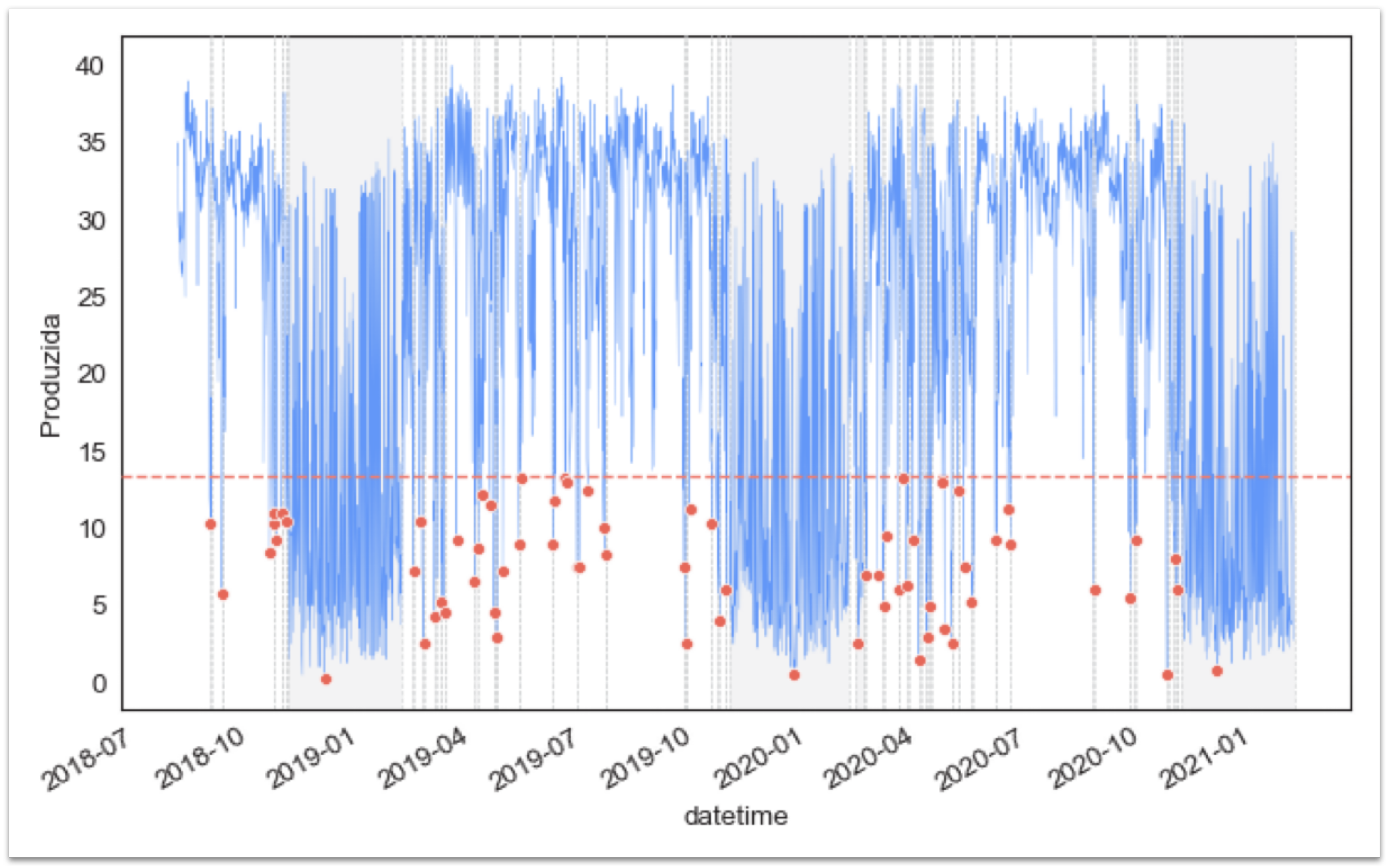
Report: From a total of 21,932 data points, 3656 were related to peak time production. During the peak hours, there are 3656 data points to be analyzed, with a mean production of 23.5 kwh. As suggested, the peak time hours are analyzed; thus, the timeframe ranges between 13:00 and 16:00, when the sun is the highest, below the 25th percentile of the production level. The key parameters (variables to be examined and constants) are shown in Table A1. The analysis of the examined data is described in detail in

Table 1. Descriptive statistics for production—Zarco use case 1.

Statistic	Value
Count	3656.00
Mean	29.22
Standard Deviation (std)	12.84
Minimum (min)	0
25th Percentile	18.25
Median (50%)	33.25
75th Percentile	40.25
Maximum (max)	48.50

and in Figure 2. The 25th percentile corresponds to a production level below 18.25.

4.1.2. EVA

We filtered the data to include only these timeframes. EVA was then applied using the Peaks-Over-Threshold method, focusing on data below our defined threshold. This threshold was set to capture the lowest 25% of production values, determined after statistical analysis of the data. To analyze the extreme value distribution, we fitted the data to a Generalized Pareto Distribution (GPD) model.

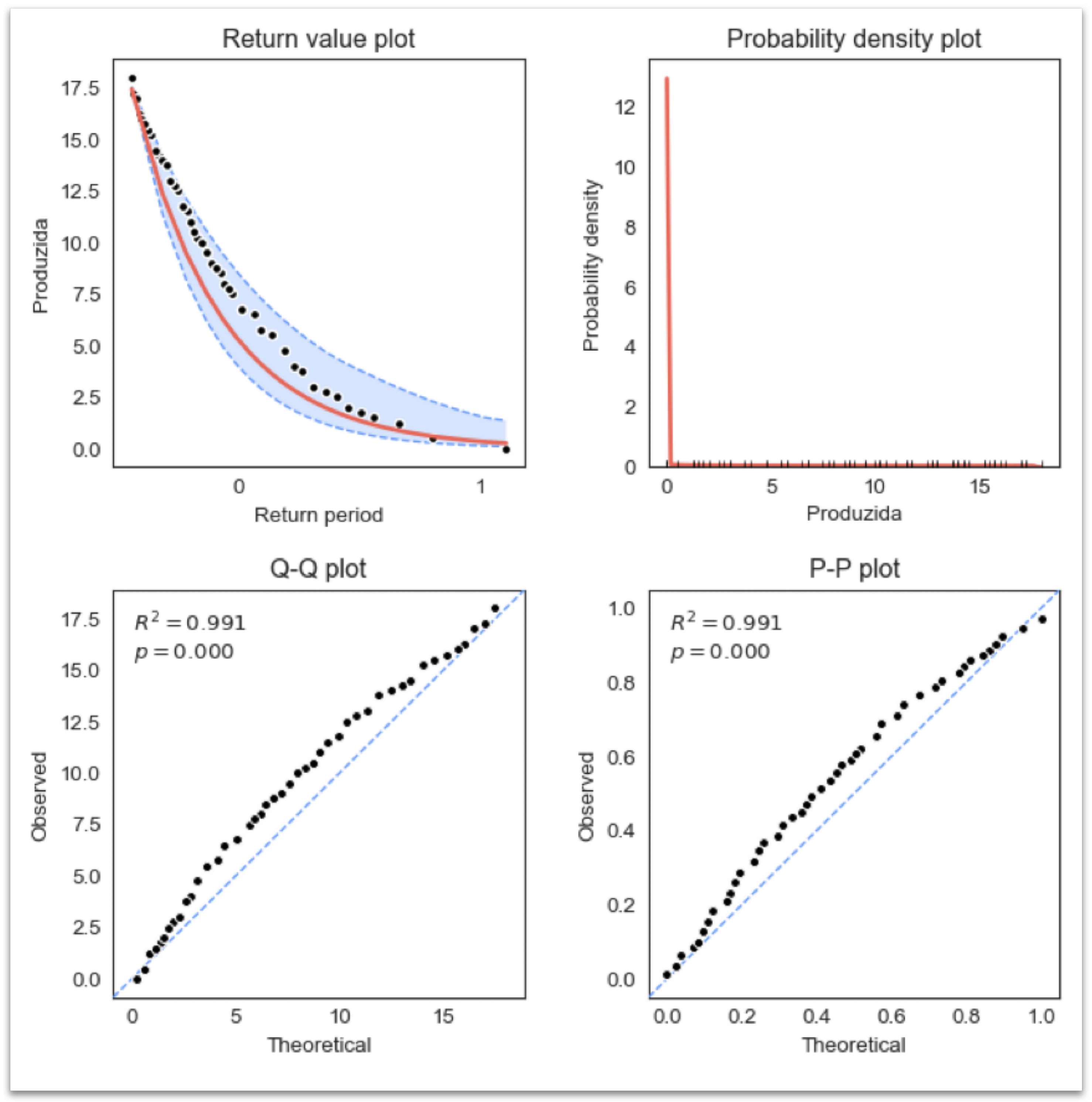
The histogram bars are not visible above the x-axis, which suggests that the observed values are so well-matched to the predicted values that the bars are hidden behind the PDF line. This would indicate an excellent fit if the theoretical model’s PDF line accurately represents the observed histogram. Return periods (in years) can be seen in

Table 2. Return periods and confidence intervals—Zarco use case 1.

Return Period	Return Value	Lower CI	Upper CI
1.00	0.35	1.66	0.11
2.00	0.15	1.31	0.04
5.00	0.05	0.75	0.00
10.00	0.02	0.58	−0.20
25.00	0.01	0.52	−0.36

.

The numbers (1, 2, 5, 10, 25, …) represent how often an event of a certain magnitude is expected to occur. For example, a 100-year-return-period event is something that, on average, we would expect to happen once every 100 years.

The return values represent the estimated magnitude of the event (e.g., production level) for each return period. The fact that these values are mostly negative suggests that we are dealing with a scenario where the focus is on low production levels or deficits. As the return period increases, the return values tend to become more negative, indicating that more extreme deficits are less frequent.

Lower and upper confidence intervals (CI) provide a range around the return value, within which the true value is expected to lie with a certain level of confidence. The confidence intervals become wider as the return period increases, indicating more uncertainty in predicting more extreme events.

One-year return period: The return value is 0.35 with a CI of [ 1.66, 0.11]. This means that in any given year, we can expect an extremely low production level of around 0.35 during peak hours, with a reasonable range of uncertainty between 1.66 and 0.11, and based on our analysis approximating 0 after 5 years.

As can be seen in the return value plot in Figure 3, the data are well fitted within the distribution; thus, the model is more reliable in predicting low production levels, allowing for more confidence in the model’s predictive capabilities.

The theoretical $R^2$ value of 0.997 and p-value of 0.000 confirm the model’s reliability in predicting the cumulative probabilities of low-production events, as shown in the plots in Figure 3, suggesting a good fit.

4.1.3. Circumstance Analysis

Applying the DISC thresholding, we extract the significant differences in correlations between the extremely low production and the normal production in the analyzed sample of peak time ranges (

Table 3. Statistical summary of weather and production data for “Zarco” use case 1.

[Zarco]	v1	v2	v3	v4	v5	v6	v7
Count	−3586.00	−3586.00	−3586.00	−3586.00	−3586.00	−3586.00	−3586.00
Mean	10.02	−1.55	27.84	0.78	−204.85	73.64	−19.82
Min	23.00	5.00	0.00	3.00	32.30	20.64	0.00
25%	9.00	1.00	22.00	1.00	−147.80	63.51	−12.75
50%	6.00	−1.00	50.50	1.00	−237.93	113.13	−23.50
75%	14.00	−3.00	38.75	0.00	−339.21	104.32	−26.25
Max	−4.00	−15.00	0.00	−15.00	−106.84	−11.46	−30.50
Std	−0.81	−2.18	1.71	−0.52	−57.07	8.25	−7.55

).

Following, the relevant information, the extremes are extracted to be used for benchmarking and comparison with a second use case to be analyzed in the next section.

4.2. EVDBM Application Use Case 2: “João” Data

4.2.1. Data Synthesis

Report: From a total of 21,908 data points, 3656 were related to peak time production. During the peak hours, there are 3652 data points to be analyzed, with a mean production of 23.5 kwh (

Table 4. Descriptive statistics for production—“João” use case 2.

Statistic	Value
Count	3652.00
Mean	23.80
Standard Deviation (std)	11.51
Minimum (min)	0.25
25th Percentile	13.43
Median (50%)	28.75
75th Percentile	33.75
Maximum (max)	40.00

). As suggested, the peak time hours are analyzed; thus, the timeframe ranges between 13:00 and 16:00, when the sun is the highest, below the 25th percentile of the production level. The key parameters (variables to be examined and constants) are shown in Table A1. The analysis of the examined data is described in detail in Table 1. The 25th percentile corresponds to a production level below 13.43 (Figure 4).

4.2.2. EVA

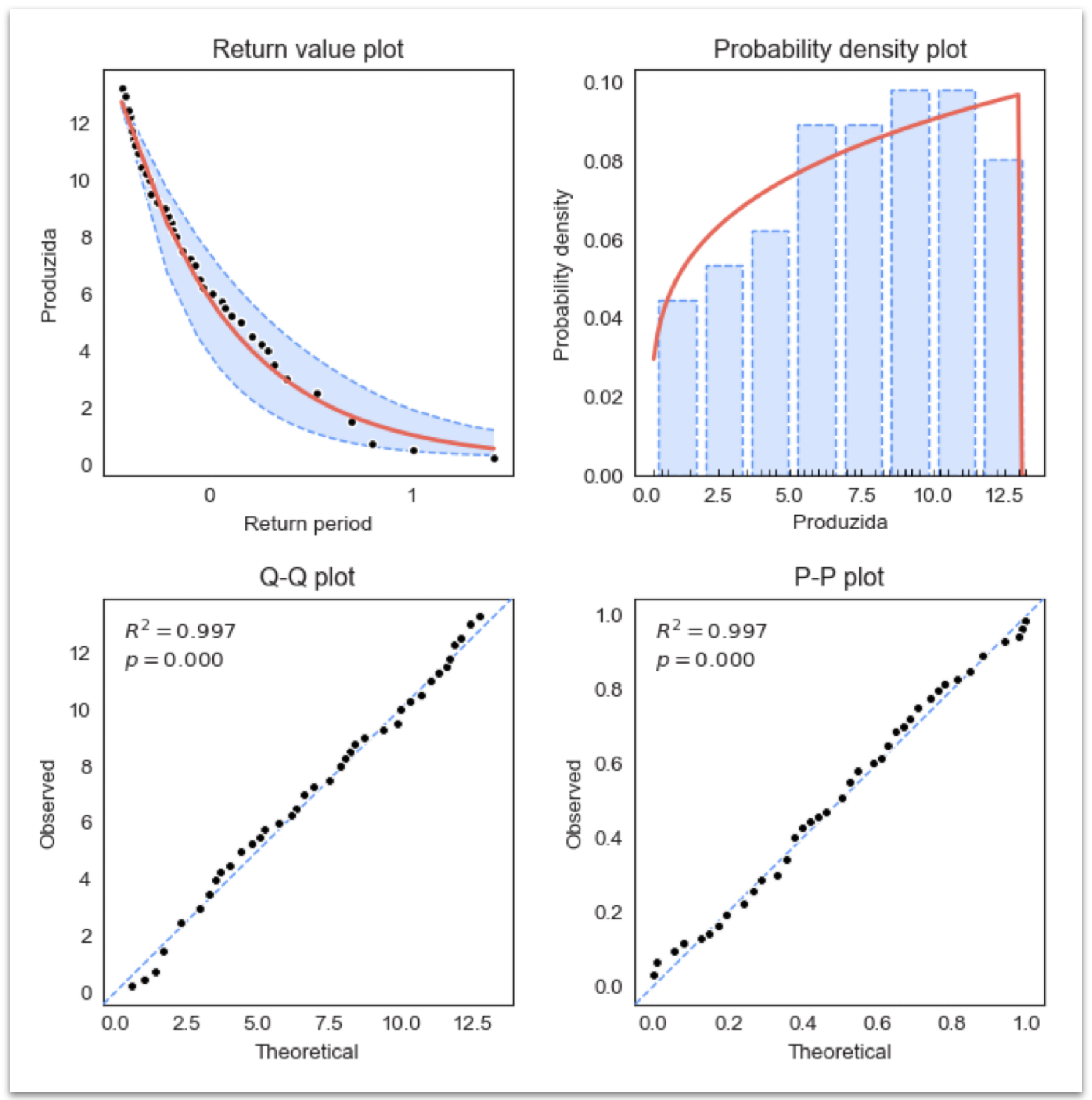
Following the previous approach we filter the data as per the time range under the chosen percentile and apply EVA. As can be seen in the return value plot in Figure 5, the data are well fitted within the distribution; thus, the model is more reliable in predicting low production levels, allowing for more confidence in the model’s predictive capabilities.

Return periods (in years) can be seen in

Table 5. Return periods and confidence intervals—João use case 2.

Return Period	Return Value	Lower CI	Upper CI
1.00	1.05	1.96	0.49
2.00	0.66	1.34	0.35
5.00	0.39	0.91	0.18
10.00	0.28	0.81	−0.06
25.00	0.20	0.72	−0.23

. One-year return period: The return value is 1.05 with a CI of [1.96, 0.49]. This means that in any given year, we can expect an extremely low production level of around 1.05 during peak hours, with a reasonable range of uncertainty, significantly higher than the observed production of use case 1.

4.2.3. Circumstance Analysis

The Statistical summary of weather and production data of the “João” use case can be seen in

Table 6. Statistical summary of weather and production data—“João” use case 2.

[João]	v1	v2	v3	v4	v5	v6	v7
Count	−3583.00	−3583.00	−3583.00	−3583.00	−3583.00	−3583.00	−3583.00
Mean	11.32	−1.81	30.48	0.48	−194.70	50.41	−16.33
Min	23.00	5.00	0.00	4.00	1.19	3.59	0.00
25%	11.00	0.00	27.00	1.00	−100.30	52.25	−8.44
50%	9.00	−1.00	57.00	1.00	−239.32	79.61	−21.25
75%	12.00	−3.00	38.00	−1.00	−342.23	65.87	−23.50
Max	−1.00	−16.00	0.00	−3.00	−86.26	−26.15	−26.75
Std	−1.83	−2.28	0.04	0.35	−52.86	0.52	−7.94

.

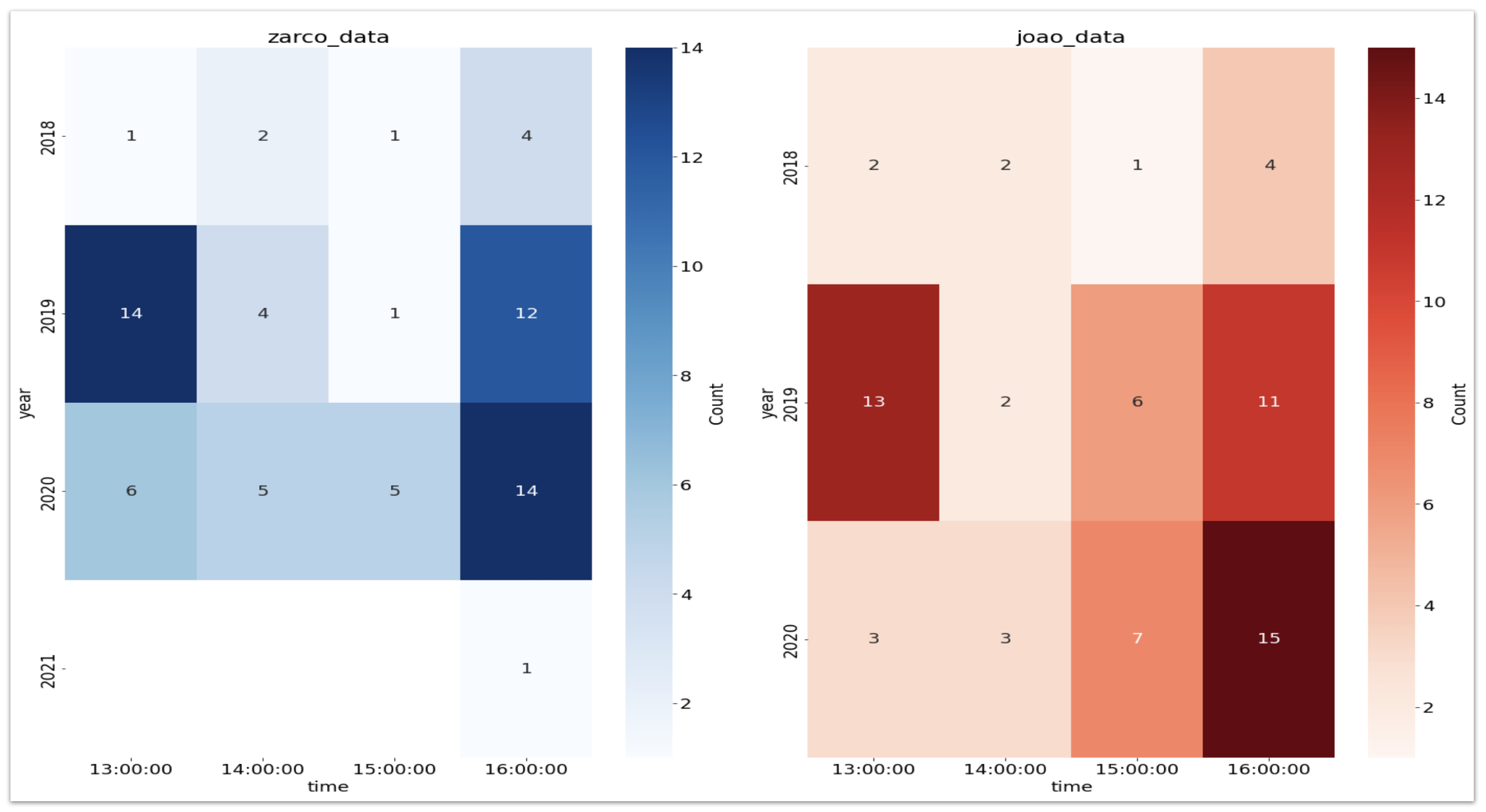
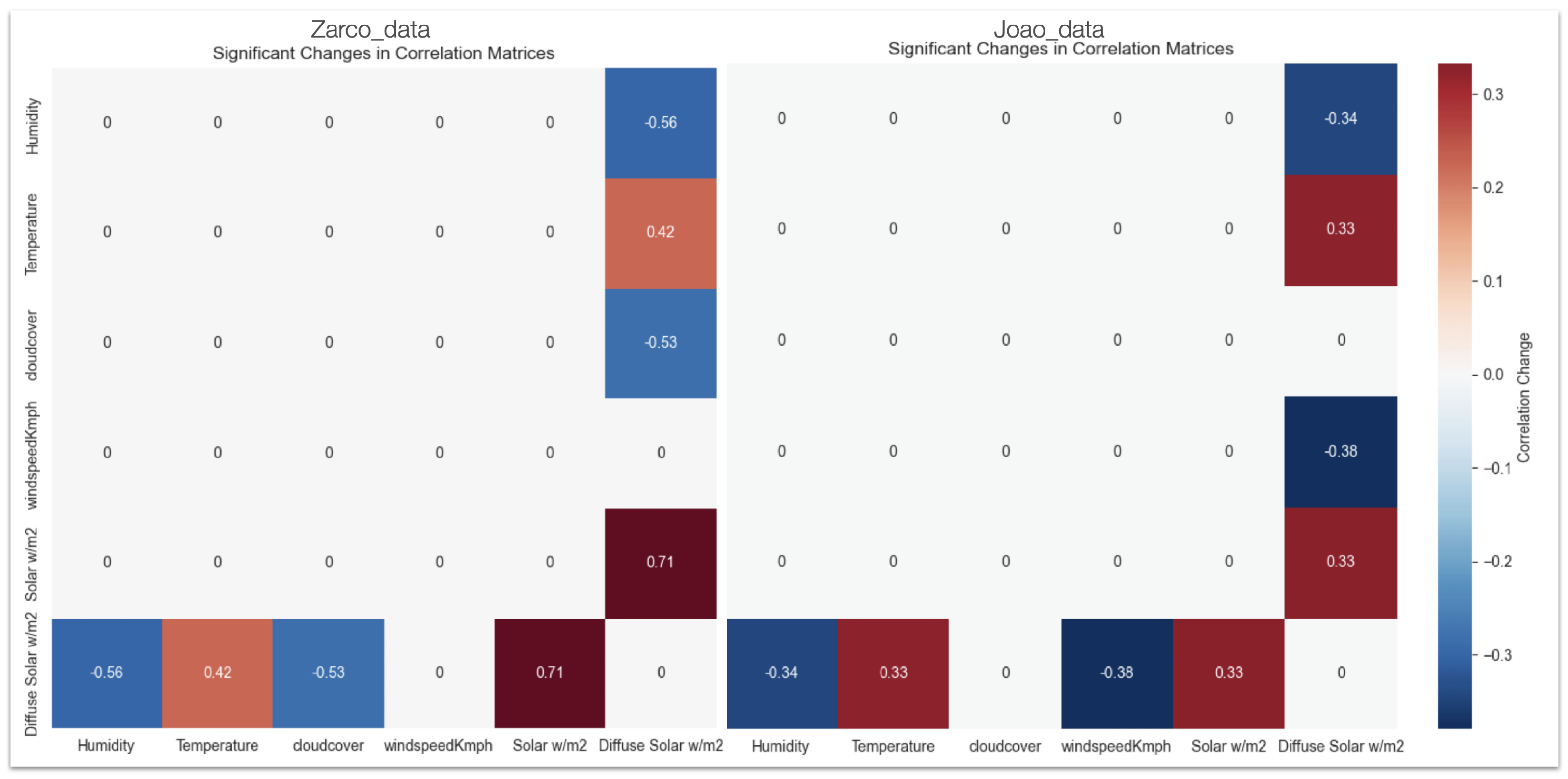
Applying the DISC thresholding, we extract the significant differences in correlations between the extremely low production and the normal production in the analyzed sample of peak time ranges (Table A1). As can be seen in Figure 6, significant differences are identified, for example between humidity and diffuse solar w/m² (HNN), and temperature and diffuse solar (HPC), for $\mathsf{\Delta }{\rho }_{ij}={\rho }_{ij}^{\mathrm{extreme}}-{\rho }_{ij}$. For the Zarco data, a significant positive correlation ($+0.71$) was observed between solar w/m² and diffuse solar w/m². Additionally, there were significant negative correlations of diffuse solar w/m² with humidity ($-0.56$) and cloud cover ($-0.53$).

In the case of the João data, a positive correlation ($+0.33$) was found between solar w/m² and diffuse solar w/m². Furthermore, diffuse solar w/m² showed negative correlations with humidity ($-0.34$) and WindspeedKmph ($-0.38$). The differences in the magnitude of correlations between Zarco and João are evident. For example, “Solar w/m²” and “Diffuse Solar w/m²” have a stronger correlation in Zarco ($+0.71$) than João ($+0.33$). Despite these differences, the DISC-thresholding algorithm isolates significant changes relative to their respective normal scenarios. This ensures that the correlation structure is normalized within each farm’s dataset, making it comparable across farms during the weight shifting optimization process.

Calculated as:

$$\mathsf{\Delta }T=T\left(x\right)-T\left(y\right),\mathsf{\Delta }\overline{v}={\overline{v}}_{\mathrm{extreme}}-{\overline{v}}_{\mathrm{normal}}$$

(11)

4.3. Benchmarking

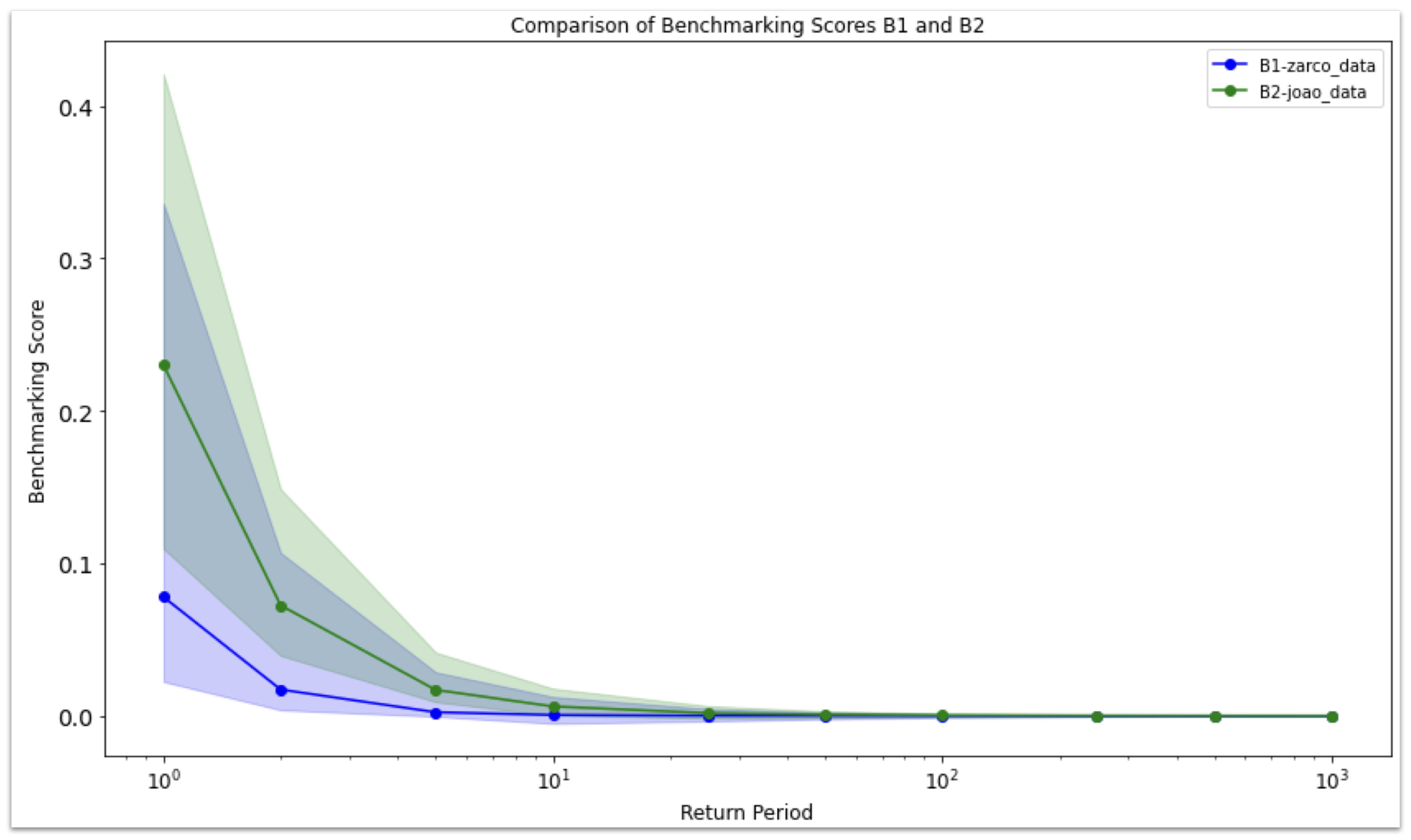
In this section we extract the benchmarking score applying the methodology described in the previous section and plot the results to highlight the differences between the two examined scenarios. Figure 7 shows that for relatively similar cases, distribution per year is about the same using the EVA-Driven Weighted Benchmarking Algorithm.

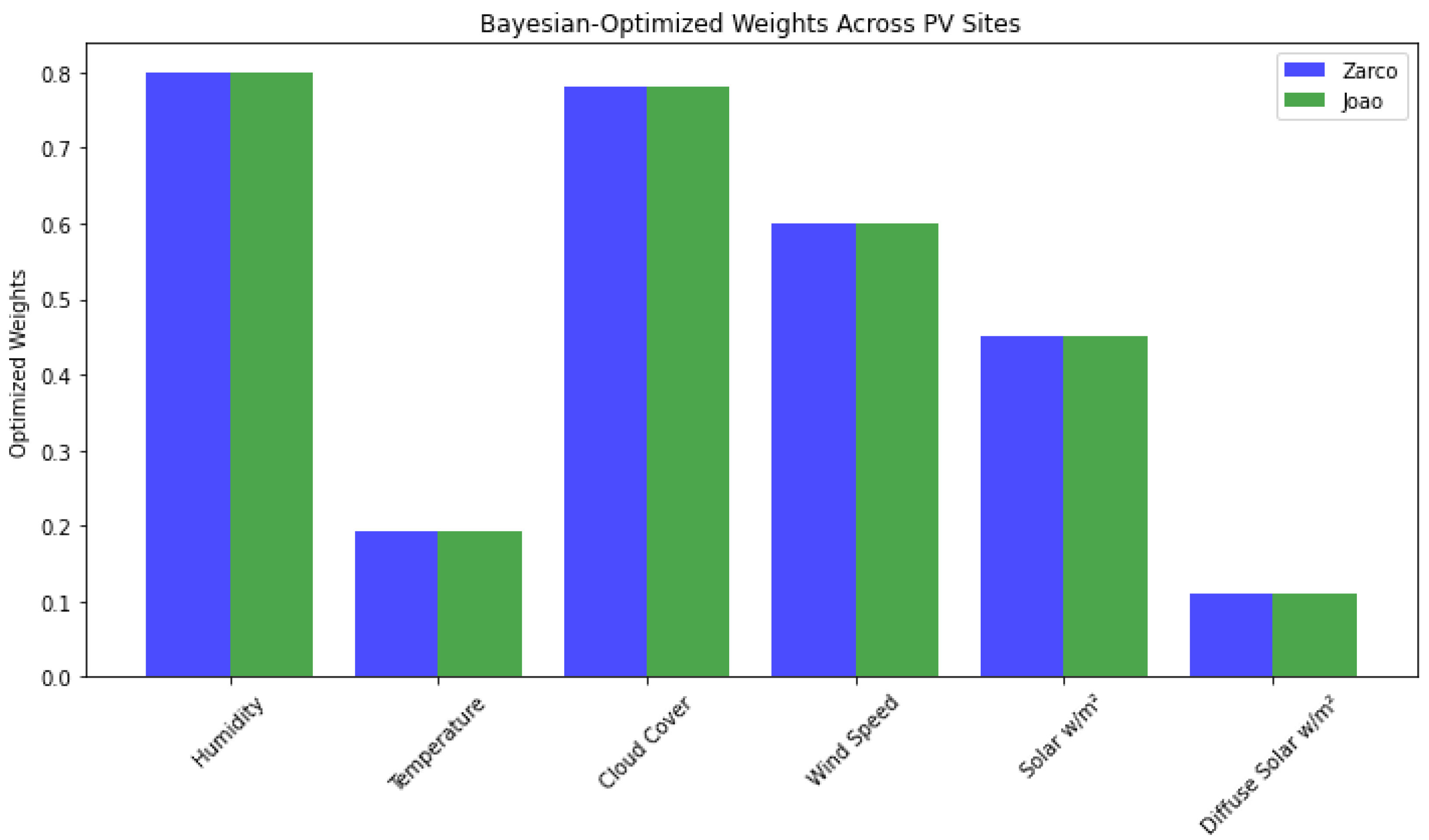
We applied grid-search weight shifting to define the optimal weights for $R^2$, presented in

Table 7. Expertly curated weights for each variable.

Variable	Suggested Weight ${\mathit{w}}_{\mathit{i}}$
Humidity (v1)	$w_1=0.05$
Temperature (v2)	$w_2=0.1$
Cloud Cover (v3)	$w_3=0.1$
Windspeed (v4)	$w_4=0.05$
Solar (Radiation) (v5)	$w_5=0.3$
Diffuse Solar (v6)	$w_6=0.2$

. Solar radiation is given the highest weight because of its dominant influence on PV performance. Cloud cover and diffuse solar radiation are also heavily weighted, reflecting their significant roles, especially during low-production periods. Temperature, windspeed, and humidity have lower weights, as their impacts are secondary but still important to consider. The normalized, weighted and scaled benchmarking scores, following the methods described, are plotted in Figure 8 and Figure 9.

A high benchmarking score suggests that the combination of environmental conditions has a greater impact on driving the system toward extreme low production. A high score implies that the system (PV plant) is more sensitive or vulnerable to these environmental factors under extreme conditions. The higher score indicates that extreme low production is likely to occur when these specific conditions are met, showing a greater dependency on or sensitivity to adverse conditions. Thus, a higher score indicates less resilience to environmental variations.

Since B2 has the highest EVDBM score it is clear that B2 (João plant) is more sensitive to adverse conditions and is less resilient against fluctuations in related circumstances.

4.4. Statistical Validation and Significance Testing

To assess whether the performance gains achieved by the proposed Extreme Value Distribution-Based Model (EVDBM) were statistically significant relative to the baseline Extreme Value Analysis (EVA), a comprehensive statistical validation was conducted.

Three complementary tests were applied: (i) Fisher’s r-to-z transformation to examine correlation structure differences; (ii) paired t-tests on absolute residuals to evaluate average error reductions; and (iii) Kolmogorov–Smirnov (KS) tests to compare the distributional characteristics of model residuals.

• Fisher’s r-to-z transformation compares the correlation coefficients between observed and predicted values to test whether EVDBM modifies the dependency structure captured by EVA.
• Paired t-test on absolute residuals assesses whether EVDBM achieves a statistically significant reduction in average prediction error magnitude compared to EVA.
• Kolmogorov–Smirnov (KS) test evaluates whether the distributional form of residuals differs between models, indicating potential systematic bias or heteroscedasticity.

Each model variant (EVDBM, EVDBM with grid-search weight optimization and EVDBM with Bayesian weighting) was compared against the EVA baseline using these tests across two photovoltaic datasets: Zarco and João. In addition to classical error metrics (MAE, MSE), a correlation-based $R_{corr}^2$ metric was computed as the squared Pearson correlation between standardized observed and predicted extreme values, capturing shape similarity rather than variance alone (

Table 8. Comparative performance and statistical significance of EVA and EVDBM variants for the Zarco and João datasets. Significant p-values (<0.05) from paired t-tests are shown in bold.

Dataset	Model	MAE	MSE	${\mathbf{R}}_{\mathbf{corr}}^2$	${\mathit{r}}_{\mathit{baseline}}$	${\mathit{r}}_{\mathit{model}}$	${\mathit{p}}_{\mathit{Fisher}}$	${\mathit{p}}_{\mathit{t}\text{-}\mathbf{test}}$	${\mathit{p}}_{\mathit{KS}}$	Significant?
Zarco	EVA	1.2031	1.8208	0.0080	0.0896	0.0896	1.0000	–	1.0000	No
	EVDBM	1.1716	1.8320	0.0071	0.0896	0.0840	0.9922	0.1011	1.0000	No
	EVDMBweights	1.1716	1.8320	0.0071	0.0896	0.0840	0.9922	0.1276	1.0000	No
	EVDBMbayes	1.1716	1.8320	0.0071	0.0896	0.0840	0.9922	0.1173	1.0000	No
João	EVA	1.1939	1.8143	0.0086	0.0929	0.0929	1.0000	–	1.0000	No
	EVDBM	1.1884	1.7515	0.0154	0.0929	0.1242	0.9561	0.0013	0.9895	Yes
	EVDMBweights	1.1884	1.7515	0.0154	0.0929	0.1242	0.9561	0.0074	0.9895	Yes
	EVDBMbayes	1.1884	1.7515	0.0154	0.0929	0.1242	0.9561	0.0041	0.9895	Yes

).

For the Zarco dataset, results show that EVDBM achieved marginal improvements in mean absolute error (−2.6%) compared with EVA, although none of the differences were statistically significant ($p>0.1$ across all tests). The correlation structure between observed and modeled extremes remained nearly identical, suggesting that the dataset’s limited tail variability constrains detectable performance differences.

In contrast, for the João dataset, all EVDBM variants consistently reduced prediction errors (MAE and MSE) and achieved higher correlation-based $R_{corr}^2$ values relative to EVA. Paired t-tests indicated statistically significant reductions in absolute error for EVDBM, EVDBMweights, and EVDBMbayes ($p<0.01$), confirming that the improvements are not due to random variation. Fisher’s r-to-z and KS tests yielded non-significant results ($p>0.95$), implying that the improvements stem from lower error magnitudes rather than a change in the correlation or residual distributional structure. These findings support the robustness of EVDBM under datasets exhibiting stronger tail behavior, such as João, where the optimization and weighting mechanisms lead to meaningful predictive gains. The results also emphasize that, while the performance gains may appear modest in absolute terms, their statistical significance indicates enhanced reliability of the model’s predictions under extreme conditions. Consequently, EVDBM can be viewed as a more stable and generalizable framework for extreme photovoltaic event modeling, with performance that scales with the degree of nonlinearity and tail complexity in the data.

To complement the statistical tests of significance, a distributional analysis was performed by comparing the quantile-to-quantile alignment between observed and modeled extremes (Figure 10). This visualization provides an interpretable view of how well each model reproduces the empirical distribution of photovoltaic extremes across quantile levels. The corresponding correlation-based $R_{corr}^2$ values for both datasets are summarized in

Table 9. Distributional alignment measured by $R_{corr}^2$ between empirical and modeled quantile functions.

Model	Zarco	João
EVA	0.900	0.952
EVDBM	0.928	0.976
EVDMBweights	0.928	0.976
EVDBMbayes	0.928	0.976

, confirming the consistency of EVDBM performance across quantiles.

Figure 10 illustrates the empirical–model quantile correspondence for the João and Zarco datasets. The black curve denotes the observed empirical quantiles, while the colored lines correspond to modeled quantiles from EVA and the proposed EVDBM variants. For both datasets, EVDBM and its optimized variants (weighting and Bayesian optimization) demonstrate visibly improved tail alignment relative to EVA, with $R_{corr}^2$ increasing from 0.90 to 0.93 for Zarco and from 0.95 to 0.98 for João (Table 9). This improvement indicates that EVDBM more accurately reproduces the empirical shape of the extreme value distribution, particularly in the upper 5% quantile region.

4.5. Ablation and Computational Complexity Analysis

To contextualize the performance evolution of the proposed framework, a structured ablation comparison was performed. The baseline Extreme Value Analysis (EVA) captures statistical extremes from univariate distributions without contextual weighting or multi-factor consideration. The proposed Extreme Value Distribution-Based Model (EVDBM) introduces multi-variable benchmarking via weighted normalization of related circumstances (e.g., solar irradiance, humidity, windspeed), while the EVDBM + XAI variant extends the model with explainable scoring metrics and correlation heatmaps ($\mathsf{\Delta }{\rho }_{ij}$) to guide model-driven decision support.

The ablation sequence (

Table 10. Naive ablation comparison among baseline EVA, EVDBM, and EVDBM + XAI. The scoring dimension refers to the integration of the benchmarking value for explainable decision-making.

Model Variant	Inputs Considered	Scoring Logic	Explainability Layer	Distribution Fit (${\mathit{R}}_{\mathbf{corr}}^2$)	MAE	Intended Use Case
EVA (Baseline)	Single variable (extremes only)	None	None	0.90 (Zarco), 0.95 (João)	1.20–1.19	Statistical characterization only
EVDBM	Multivariate (physical drivers)	Weighted benchmark	Partial (weights)	0.93 (Zarco), 0.97 (João)	1.17–1.18	Enhanced prediction under multivariate dependence
EVDBM + XAI	Multivariate + Correlation shifts	Benchmark + XAI-driven scoring	Full ($\mathsf{\Delta }{\rho }_{ij}$, feature impact, ABCDE heatmaps)	0.93–0.97 across datasets	1.17–1.18	Decision support and model interpretability

) shows a steady increase in both distributional alignment and interpretability. While EVA provides only statistical tail estimates, EVDBM incorporates contextual dependencies through multivariate weighting, yielding consistent performance improvement in both datasets.

EVDBM + XAI further introduces an interpretable layer that integrates benchmarking scores with correlation-based diagnostics, enabling domain experts to understand the drivers of extreme deviations. The incremental increase in complexity is minimal compared to the added decision-making capacity.

From a computational perspective (

Table 11. Algorithmic and computational complexity comparison of EVA and EVDBM variants. All models were evaluated on identical hardware under identical sampling configurations.

Model	Complexity (Big-O)	Runtime (avg)	Memory Overhead
EVA (Baseline)	$\mathcal{O}\left(n\right)$	1.0x (reference)	Low
EVDBM (Weighted)	$\mathcal{O}(n\times m)$	1.4x	Moderate
EVDBM + GridSearch	$\mathcal{O}(n\times m\times k)$	2.1x	Moderate
EVDBM + Bayesian	$\mathcal{O}(n\times m)$ (optimized)	1.7x	Moderate
EVDBM + XAI (Full)	$\mathcal{O}(n\times m)$ + XAI overhead	2.3x	Slightly higher (visual output)

), the core EVDBM process scales linearly with the number of contextual variables (m) and optimization steps (k) in grid or Bayesian search. Even in the full XAI configuration, runtime remains within approximately 2.3× the baseline EVA, maintaining suitability for real-time or near-real-time applications. The additional interpretability layer introduces only a marginal increase in memory footprint due to correlation mapping and feature attribution visualization.

5. Discussion of Results

Compared to baseline EVA, EVDBM introduces a dynamic weighting and benchmarking mechanism that captures multivariate dependencies among related variables (e.g., irradiance, humidity, temperature, and wind). Through grid search and Bayesian optimization, EVDBM adaptively adjusts variable weights to optimize the alignment between observed and modeled extremes. Across both test sites (Zarco and João), the correlation-based $R_{corr}^2$ rose from 0.90 to 0.93 for Zarco and 0.95 to 0.98 for João (Table 9).

The quantile-to-quantile comparison plots (Figure 10) further highlight this improvement, illustrating how EVDBM and its optimized variants more accurately reproduce empirical tail distributions, particularly in the upper 5% quantile region. These enhancements demonstrate that EVDBM is not merely statistically sound but also distributionally consistent, yielding smoother and more stable projections across extreme-value quantiles.

The EVDBM framework was statistically validated using multiple significance tests (Table 8). For both datasets, Fisher’s r-to-z, paired t-tests, and Kolmogorov–Smirnov (KS) tests were applied to compare EVDBM variants against EVA. In the João dataset, EVDBM variants achieved statistically significant reductions in residual error ($p_t<0.01$), confirming the robustness of the improvement. The Zarco dataset, characterized by smoother and less volatile extremes, showed stable but not statistically significant gains ($p>0.1$), indicating that EVDBM preserves accuracy under more stationary conditions. KS tests confirmed that EVDBM did not distort the underlying distributional structure, maintaining statistical consistency with empirical residuals ($p_{KS}>0.95$ across all variants). These findings reinforce EVDBM’s robustness and generalizability, demonstrating that the model enhances tail fidelity and interpretability without compromising distributional integrity.

Although bootstrapping was initially implemented as part of the statistical validation process, it was later removed due to sampling imbalance between EVA-generated return values and EVDBM benchmarking points. The unequal sampling density introduced bias in the resampling procedure, particularly when aligning extreme quantiles across the two formulations. This limitation was explicitly addressed in the revised discussion, emphasizing that the presented statistical tests (Fisher’s r–to–z, paired t-test, and KS test) provide a more stable and interpretable basis for assessing model significance. Future work will explore bootstrapped cross-validation under equalized sampling conditions to further quantify uncertainty and robustness across multiple extreme value regimes.

The ablation analysis (Table 10) shows that the progression from EVA to EVDBM to EVDBM + XAI yields cumulative gains in interpretability, predictive stability, and decision value. While EVA efficiently estimates univariate extremes, it lacks explanatory capability. EVDBM extends this by introducing weighted benchmarking across correlated drivers, enhancing both accuracy and contextual understanding. The XAI-enhanced variant (EVDBM + XAI) further integrates DISC-based correlation maps ($\mathsf{\Delta }{\rho }_{ij}$) and ABCDE heatmap scoring, offering visual interpretability of the factors driving extreme behavior. Together, these layers allow EVDBM not only to predict extreme events but also to explain and justify their occurrence—an essential capability for informed decision-making in energy systems.

5.1. Conclusions

The DISC-thresholding algorithm identifies and isolates significant shifts in variable correlations between normal and extreme scenarios. This provides interpretability, as it allows domain experts to understand which relationships between variables (e.g., “Solar w/m²” and “Diffuse Solar w/m²”) become more critical under extreme conditions. Also, it provides context-specific insights; by highlighting variable dependencies within each farm, DISC enables the identification of drivers of extreme behavior, even when datasets differ structurally.

Identical weights result from shared structural dependencies (e.g., “Solar w/m²” and “Diffuse Solar w/m²”) highlighted by DISC. This demonstrates that while the magnitude of correlation shifts differs, the underlying variables driving extreme behavior remain consistent. DISC helps explain why the same variables dominate the optimization process across datasets: they exhibit the most significant and meaningful changes under extreme conditions.

Global and Local XAI in EVDBM

• Global Explainability: DISC and grid search explain which variables (e.g., “Solar w/m²” and “Diffuse Solar w/m²”) are critical across all farms, offering insights into general drivers of extreme (low) production levels.
• Local Explainability: Heatmaps from DISC provide farm-specific insights, explaining unique correlation patterns (e.g., the stronger impact of “Humidity” in Zarco compared to João).

DISC ensures transparency by producing intuitive and interpretable outputs, such as heatmaps and correlation shifts, alongside the associated benchmarking scores with optimized weights. These outputs provide clear and actionable explanations for extreme production behaviors, enhancing the overall explainability of the framework. The ability to interpret and trust extreme event predictions is critical for energy grid operators, policymakers, and infrastructure planners. EVDBM ensures that predictions are not only accurate but also interpretable, enabling better real-time responses to energy fluctuations and long-term strategic planning.

The outputs of EVDBM directly align with ongoing EU and national policy frameworks that emphasize resilience assessment, risk-aware planning, and explainable energy analytics. In particular, the framework supports policy objectives outlined in the European Green Deal and the EU Strategy on Adaptation to Climate Change, which call for transparent, data-driven tools capable of quantifying vulnerability and improving system resilience under extreme environmental conditions. By providing interpretable benchmarking indicators—such as DISC-based correlation maps, resilience indices, and dynamic return-level evaluations—EVDBM delivers actionable intelligence for grid operators, regulators, and policymakers. These outputs facilitate compliance with energy resilience directives and assist in defining evidence-based investment strategies, infrastructure priorities, and early-warning thresholds for critical energy assets. In doing so, EVDBM bridges the gap between technical analysis and operational policy needs, promoting a measurable, explainable foundation for risk-informed decision-making in renewable energy systems.

5.2. Limitations and Future Work

The main limitations of this work to be addressed are the following:

• Sensitivity to Data Quality and Availability: The accuracy of EVDBM depends on the quality, frequency, and representativeness of historical data, especially under extreme conditions. Sparse or incomplete recordings of rare events can lead to biased parameter estimation and less reliable benchmarking scores. This limitation is particularly relevant for small-scale or newly commissioned systems, where the empirical tail behavior is still underdeveloped.
• Partial Assumption of Stationarity: While the model accounts for dynamic relationships through the DISC-thresholding and adaptive weighting mechanisms, it still assumes partial stationarity in the long-term behavior of the underlying variables. Structural shifts—such as climate trends, technological upgrades, or policy interventions—can alter the probability and intensity of future extremes, potentially reducing the validity of historical benchmarks.
• Dependence on Model Calibration and Optimization: The performance of EVDBM is influenced by the configuration of its optimization routines (grid or Bayesian search). Inadequate tuning ranges or limited computational budgets may lead to suboptimal weight identification, especially in high-dimensional correlation spaces. Although this is mitigated by the explainable design, calibration sensitivity remains a factor in achieving consistent performance.
• Interpretability–Performance Trade-off: The inclusion of the DISC and XAI layers enhances transparency but increases model complexity and the number of intermediary parameters. In certain scenarios with low variance or weak correlations, these layers may add interpretative noise rather than clear explanatory value.
• Computational Overhead for Real-Time Deployment: Although EVDBM maintains near-linear computational scaling, the additional explainability modules (DISC computation, correlation heatmaps, and ABCDE scoring) introduce extra processing steps. This can be limiting in real-time or embedded energy forecasting systems with strict latency requirements.
• Scope of Validation: The present evaluation focused on two photovoltaic datasets. Broader validation across domains (e.g., hydrology, finance, or climate risk) and larger, higher-resolution datasets is required to confirm generalizability and to refine the sensitivity of the statistical significance tests.

In our future work, we intend to expand the application of EVDBM within the energy sector, particularly in areas where highly specific decision-making can optimize energy management and resilience planning. This includes forecasting extreme fluctuations in renewable energy generation, optimizing grid balancing strategies, and improving predictive maintenance for photovoltaic (PV) systems. Additionally, we are working on integrating the EVDBM algorithm for scenario-based analysis, enabling what-if simulations and advanced risk-management applications in energy trading, storage optimization, and climate impact assessments. By incorporating a more dynamic approach to extreme event prediction, we aim to further enhance adaptive energy strategies and long-term sustainability planning. Future research will extend this framework through comparative evaluations against other predictive and analytical paradigms, including quantile regression, Generalized Pareto and Bayesian hierarchical models, and machine-learning-based extreme value predictors. Additional work will explore the integration of non-stationary EVA formulations, uncertainty propagation through Bayesian updating, and hybrid deep learning–EVA architectures for dynamic forecasting. Moreover, expanding the validation of EVDBM across multi-domain datasets—such as climate risk, hydrology, and financial extremes—will help assess its generalizability and refine its explainability under diverse operational conditions.