Abstract
Indoor localization techniques operate independently of Global Navigation Satellite Systems (GNSSs), which are primarily designed for outdoor environments. However, integrating indoor and outdoor positioning often leads to inconsistent and delayed location estimates, especially at transition zones such as building entrances. This paper develops a probabilistic transition detection algorithm to identify indoor, outdoor, and transition zones, aiming to enhance the continuity and accuracy of positioning. The algorithm leverages multi-source sensor data, including WiFi Received Signal Strength Indicator (RSSI), Bluetooth Low-Energy (BLE) RSSI, and GNSS metrics such as carrier-to-noise ratio. During transitions, the system incorporates Inertial Measurement Unit (IMU)-based tracking to ensure smooth switching between positioning engines. The outdoor engine utilizes a Kalman Filter (KF) to fuse IMU and GNSS data, while the indoor engine employs fingerprinting techniques using WiFi and BLE. This paper presents experimental results using three distinct devices across three separate buildings, demonstrating superior performance compared to both Google’s Fused Location Provider (FLP) algorithm and a GPS.
1. Introduction
Accurate and continuous location tracking has become a fundamental requirement for a wide range of applications, including navigation, asset management, emergency response, and smart city services. While outdoor positioning is largely achieved by satellite-based systems such as GPSs, these signals are often unreliable or unavailable indoors due to signal attenuation and multi-path effects. Conversely, indoor positioning systems relying on technologies such as WiFi, Bluetooth, or inertial sensors typically lack coverage or accuracy once users move outside. This fragmentation creates significant challenges for providing seamless, uninterrupted tracking as users transition between indoor and outdoor environments [1].
Recent advances in sensor fusion, machine learning, and environmental awareness have enabled the development of integrated solutions that aim to bridge this gap. Systems such as IODetector in [2] and SUNS in [3] demonstrate the potential of combining data from multiple sources including GNSS, Wi-Fi, Bluetooth, and inertial sensors to achieve robust, user-friendly, and seamless tracking across diverse environments. However, despite these advances, ensuring high accuracy, low latency, and energy efficiency during indoor–outdoor transitions remains a complex problem, particularly in dynamic or infrastructure-limited settings.
This paper proposes a seamless tracking algorithm specifically designed for Google Android smartphones for the continuous and uninterrupted tracking of a person or object as they move between indoor and outdoor environments, maintaining smooth and continuous trajectory estimation [4,5,6]. The proposed positioning system integrates measurement data from three primary sources: WiFi RSSI and BLE RSSI, inertial sensors (IMUs), and a GNSS. The user’s environmental state, categorized as indoor, transition, or outdoor, is inferred using a combination of RSSI values, GNSS satellite information, and previously estimated positions. For indoor localization, the system employs a hybrid of WiFi-based fingerprinting and AI-augmented IMU tracking [7], with particle filtering applied in the post-processing stage. In contrast, the outdoor localization engine combines GNSS and AI-IMU data through an extended Kalman Filter (EKF) for robust estimation. During transitional phases, where both WiFi and GNSS signals tend to be unreliable, the system switches to AI-IMU tracking with a particle filter, operating without external signal sources.
Accurately detecting the transition zone is crucial for seamless tracking, as the handover strategy, which is responsible for determining whether the device is in an indoor, outdoor, or transition state, significantly impacts overall tracking performance. The classification into these three states is based on RSSI signals, the previously estimated position, and GNSS signals. Notably, the RSSI signal model is derived using a neural network activation function. While machine learning models typically require training data, which are often gathered through supervised methods such as fingerprinting [8], this paper adopts an unsupervised data collection approach. In our method, the device collecting RSSI signals operates freely, without constraints such as being held in a fixed position. An overview of the entire positioning process is illustrated in Figure 1.
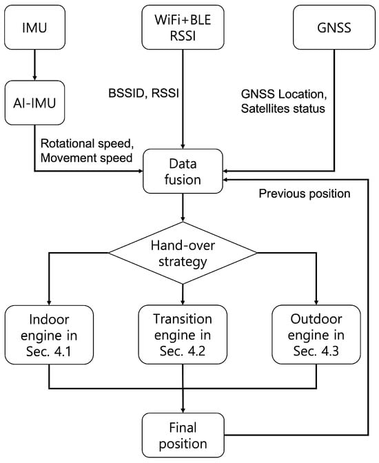
Figure 1.
Overview of the proposed seamless indoor–outdoor localization.
This paper is structured as follows: Section 2 introduces some related works. Section 3 presents the handover strategy. Section 4 describes the separated positioning engines for indoor, transition, and outdoor. The experimental results and real-time verification results of the proposed model are analyzed in Section 5. The research directions and conclusions are proposed in Section 6.
2. Related Works
Recent research on indoor–outdoor seamless tracking has focused on integrating various sensors and positioning systems such as GNSS, Bluetooth, WiFi, and IMU using advanced fusion algorithms such as federated filters and machine learning. Key trends include smooth transitions at indoor–outdoor boundaries, high accuracy, real-time performance, and minimal infrastructure requirements [9,10,11,12,13].
Ref. [14] proposes a method to automatically detect and distinguish indoor, outdoor, and transition zones by analyzing the time series of GNSS error statistics. This helps decision-making process between visual–inertial odometry and GNSS-based trajectory estimation. Ref. [15] presents a hybrid positioning system that fuses Bluetooth Angle of Arrival and GNSS signals, which utilizes commercial tracking devices to simultaneously transmit Bluetooth and receive GNSS signals.
The hidden Markov model and Bayesian inference-based indoor–outdoor transition tracking in [16] overcome the limitations of threshold-based sensor switching by employing hidden Markov models (HMMs) and Bayesian inference for seamless indoor–outdoor tracking. This algorithm takes advantage of the continuous-time nature of HMMs for smooth and accurate localization during transitions.
The adaptive federated filter-based approach in [17] integrates IMU, GNSS, and indoor positioning systems using an adaptive federated filter. It enables multi-target indoor tracking and identification without additional hardware as well as provides stable and smooth tracking throughout the entire indoor–outdoor trajectory.
A navigation system [3] was designed to provide seamless and ubiquitous positioning for users as they move between indoor and outdoor environments. It enhances environmental awareness by integrating multiple sensing technologies, such as GPS, WiFi, and inertial sensors, to accurately detect whether the user is indoors or outdoors. The IODetector in [2] detects whether a mobile device is indoors, semi-outdoor, or outdoors. It combines data from multiple sensors such as GPS, WiFi, Cellular RSS, IMU, proximity, light, and magnetic field sensors. To enable light and magnetism detectors, certain conditions must be met. For instance, the tracked device should be free from the interference caused by external magnetic sources, and the difference in lighting between indoor and outdoor environments should be significant.
Most related works on seamless indoor–outdoor tracking have focused on handover strategies within the transition zones between environments. Unlike other works, this paper proposes unsupervised data collection to detect the transition zone using a softmax activation function as a machine learning approach. Fused data also include multi-sensor as well as previously estimated position information.
3. Handover Strategy Based on Three State Density Functions
The positioning environment is categorized into three distinct states: indoor, transition, and outdoor, as illustrated in Figure 2. The transition state is defined symmetrically around the transitional features such as doors or building entrances that serve as physical boundaries between indoor and outdoor areas. When a state change is detected, a handover strategy is triggered, transferring both the latest estimated position and the corresponding error covariance matrix from the current positioning engine to the next.
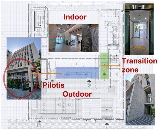
Figure 2.
One of the experimental office buildings. This building has a pilotis structure, and both sides of the exterior entrances are surrounded by walls and obstacles, making seamless tracking more challenging. There is a double-door entrance connecting the indoor and outdoor spaces, and the transition zone was selected as the area between the inner and outer doors.
A state handler continuously evaluates the probabilities for each possible state . The state with the highest probability is selected as the current operating state such that
The state probabilities are derived from three independent estimation models: an RSSI-based model, a position–distribution model, and a GNSS-based distribution model. Each model produces a probabilistic estimate for the current state, reflecting different aspects of the environment. The final state probability is calculated as a weighted sum of these individual model outputs.
The weights assigned to each model are manually tuned through empirical evaluation to achieve optimal state classification performance. This approach is necessary because each building features a unique configuration of WiFi and BLE access points, which affects , and distinct structural characteristics around transition zones, which influence . Therefore, in this paper, the weights are experimentally optimized for each environment.
3.1. RSSI Model
The RSSI model takes the WiFi and BLE scan results as the input and returns the probabilities of states. The data to train the RSSI model are obtained from the RSSI data measured while randomly walking in specific areas. The data were measured for about 3 min for each state area, with 5 s of WiFi and BLE scanning intervals.
The RSSI scan result of the WiFi and BLE accumulated for each time window of 5 s is defined as a vector of size m,
where is the scalar value of the RSSI corresponding to the ith access point (including BLE beacons) at the kth location, which is normalized from ( dBm, 0 dBm) to (0, 1). The measured RSSI values lower than dBm are considered dBm.
The autoencoder function transforms the normalized m-dimensional RSSI vector of WiFi and BLE into a dimensionality-reduced d-dimensional feature vector.
The learning model predicts the state for a given set of inputs. For the output layer, the softmax activation function was used to return estimations in the form of probabilities.
3.2. Position-Based Model
The position-based distribution model takes the estimated position as the input and returns the probabilities of states. The position-based probability of states at the kth location is an arbitrarily designed nonlinear function, which takes as inputs, where is the estimated position at the kth location, and is the position of the transition point nearest to the estimated position, as shown below.
The probability of being in a transition state increases as the estimated position approaches the transition point, reaching a value of 1 when the estimated position coincides with the transition point. The remaining probability, after accounting for the transition state, is equally distributed between the indoor and outdoor states.
3.3. GNSS-Based Model
The GNSS-based distribution model considers the carrier-to-noise density in decibels () and the number of satellites used in fix () to determine the probabilities of each state. The cases are broken into two by checking if is below 4 or not, taking into account that at least 4 satellites are required for an accurate GNSS fix. After considering the number of satellites, it takes the mean of the carrier-to-noise density () for four satellites with the highest value as the input and returns the probabilities of states at the kth location , which is also an arbitrarily designed nonlinear function, as shown below.
For the case where , rises from 0 at and reaches the highest value of 1 at , decreasing back to 1 at . starts to decrease from 1 at and reaches a minimum value of 0 at , where starts to increase from 0 until it reaches a value of 1 at .
4. Positioning Engines
4.1. Indoor Positioning Engine
In indoor environments where GNSS signals are obstructed, wireless-signal-based positioning technologies have gained significant attention. An unsupervised WiFi RSSI positioning model using a particle filter to fuse WiFi and AI-IMU location estimates for trajectory tracking was proposed in our previous work [18]. As an AI-IMU tracking model, we use RoNIN [7] in this paper.
The scanned RSSI data are dimensionality-reduced in a similar manner to Equations (3) and (4) but considering only WiFi results and thus excluding the BLE. The learning model predicts the position at a given RSSI feature vector .
The sensing frequency of the WiFi RSSI is relatively low compared to the IMU. Furthermore, the absolute location is estimated from the WiFi RSSI while the relative location is estimated from the AI-IMU. To address this issue, a particle filter was employed for the sensor fusion.
The state of the particle is defined as below:
The prior for the indoor positioning is set by the existence of a wall.
The transition function from location to k of the ith particle is modeled as below:
where and are the position and angular displacement estimations from the AI-IMU.
The likelihood for particles corresponding to the AI-IMU is defined to measure the distance error of a particle to an average, while the likelihood for the particles corresponding to the WiFi positioning model is defined to measure distance error of a particle to the estimated position from the learning model ,
where the number of particles , , and measurement error variance are manually tuned parameters.
Both AI-IMU and WiFi particles are used for the resampling step of the particle filter to compensate for the bias error of the AI-IMU estimations at the WiFi particle update.
The pseudo-code of the indoor positioning algorithm is shown below in Appendix A.
4.2. Transition Positioning Engine
The transition positioning engine is separately designated to handle areas where both WiFi and GNSS signals are unreliable. Basically, this algorithm is a particle filter with only the AI-IMU particles described earlier, with increasing error covariance for each propagation. The prior function in Equation (18) is not applied for the transition positioning engine (the prior function is always 1) since it can block estimation moving from outdoor to indoor or vice versa when the estimated position is not accurate, worsening the position error. Note that resampling process does not occur since the prior function is always 1.
The pseudo-code of the transition positioning algorithm is shown below in Appendix B.
4.3. Outdoor Positioning Engine
The GNSS fix position (, ) and the confidence interval of the position are received from the Android LocationManager API every 1 s. The AI-IMU returns the estimated moved distance and rotated angle in a 0.25 s interval. The extended Kalman filter (EKF) was used to estimate the position using those measurements in the outdoor environment.
The rotational speed (), direction angle (), movement speed v (), x position (m), and y position (m) were used as state variables, as shown below:
The initial position , is either handed over from the indoor/transition positioning engine or decided from the initial GNSS fix position.
The state-transition function and its Jacobian matrix A from the state at time t to time was modeled as below:
The prediction noise covariance matrix Q was designed as below:
The AI-IMU measurement gives the angular displacement in direction angle () and moved distance (m) for time interval (s), while the GNSS measurement gives latitude (), longitude (), and accuracy (m). The value, obtained from the Android LocationManager API, represents the range within where there is 68% probability that the true position will be found.
The measured states (, ) at time t were derived as below:
where u is a phase unwrapping function, and is an estimated speed from the differentiated GNSS position in the time domain.
The measurement noise covariance matrices and for the AI-IMU and GNSS were designed as below:
where is the accuracy obtained from the android location request, and is a weight function of the predicted speed(), the estimated speed from GNSS fix positions (), and the estimated moved distance from the transition region (), designed to increase the measurement error covariance when the position is close to the transition area or the displacement of the position from the GNSS measurement is too large compared to the estimated movement speed. The aim of this weight function is to suppress the error from the FLP measurements with a small value and a large position error, mostly due to the GNSS multi-path errors in the urban environment.
The threshold value that determines the condition in (31) was set to based on the observation of the moving speed from the AI-IMU when the device was not moving, which showed random values between and .
The noise covariance matrix of the GNSS measurement is based on the assumption that the accuracy value is from a folded normal distribution of a position error . The other coefficients were manually tuned.
The pseudo-code of the outdoor positioning algorithm is shown below in Appendix C.
5. Experimental Results
The test was conducted in three office buildings (indoor area: Maru360—140 , Keumha—220 , and Namsan Green—470 ) with three different kinds of smartphones (Samsung Galaxy S10, S20, and S21). To train the positioning model, 30 min was spent in collecting the unlabelled datasets by two people with two smartphones each (three Samsung Galaxy S21s and one Samsung Galaxy S20). The test trial was conducted by one person, and the same trajectory was repeated for three (Keumha, Namsan Green)/four (Maru360) times. The black line shows the ground truth trajectory, while the green, blue, and red lines each refer to the estimated trajectory from the proposed method, Google’s Fused Location Provider (FLP) algorithm [19], and GPS. For ground truth generation, the initial trajectory was estimated using the AI-IMU method. This trajectory was then refined by interpolating between the designated positions such as the start and end points within the time domain to produce a continuous ground truth path. Figure 3, Figure 4 and Figure 5 show examples of the experimental results compared with Google’s fused location provider API for each building.
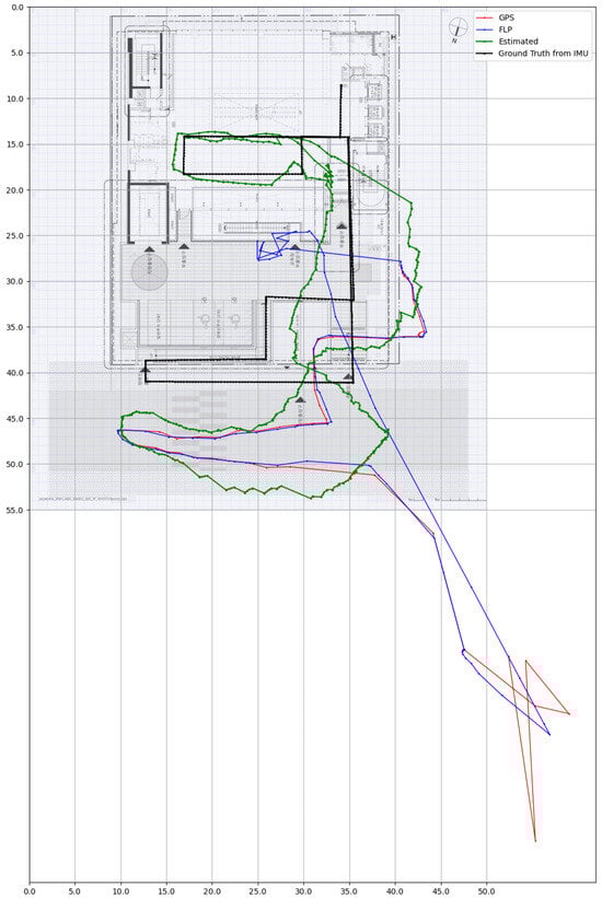
Figure 3.
Estimated trajectories compared to a GPS and Google’s FLP at Maru360.
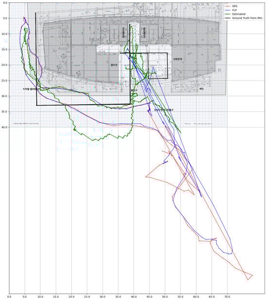
Figure 4.
Estimated trajectories compared to the GPS and Google’s FLP at Keumha.
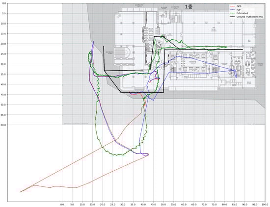
Figure 5.
Estimated trajectories compared to the GPS and Google’s FLP at Namsan Green.
The position errors were compared between the estimated trajectory, FLP, and GPS for each device. The distribution of errors is shown with box plots in Figure 6, Figure 7 and Figure 8, the box plot in the left column shows the distribution of the position errors during all trials, the box plot in the center column shows the errors between the FLP position measurement and the estimated trajectory, and the box plot in the right column shows the errors between the GPS position measurements and the estimated trajectory.
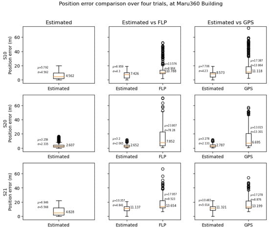
Figure 6.
Position error distribution of the estimated trajectory at Maru360 compared to the GPS and FLP.
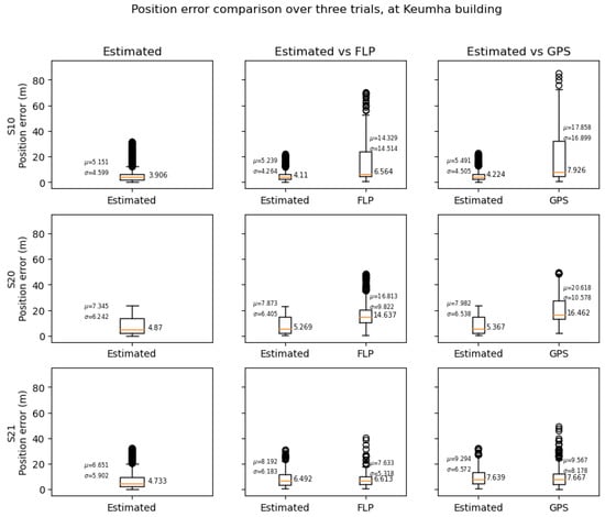
Figure 7.
Position error distribution of the estimated trajectory at Keumha compared to the GPS and FLP.
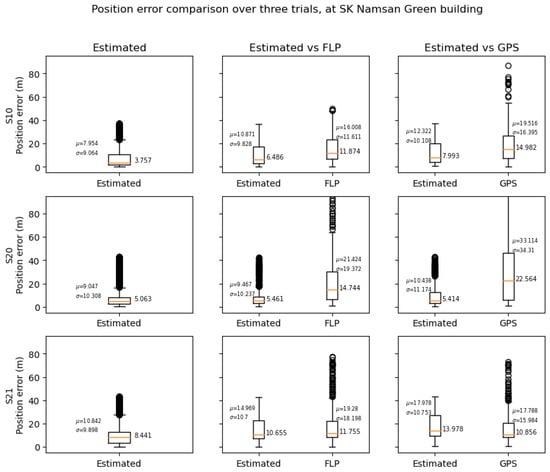
Figure 8.
Position error distribution of the estimated trajectory at Namsan Green compared to the GPS and FLP.
The estimated trajectory’s position error compared to the FLP error was calculated by interpolating the trajectory by the FLP measurement’s timestamp and then comparing it with the ground truth. Similarly, the estimated trajectory’s error compared to the GPS error was calculated by interpolating it with the GPS measurement’s timestamp and then comparing it with the ground truth.
The median, mean, and standard deviation of the errors shown in the plot are also summarized in Table 1, Table 2 and Table 3.

Table 1.
The median, mean and standard deviation of the position estimation errors over four walking scenario tests at Maru360 in meters.
Table 2.
The median, mean, and standard deviation of position estimation errors over four walking scenario tests at Keumha in meters.
Table 3.
The median, mean, and standard deviation of position estimation errors over four walking scenario tests at Namsan Green in meters.
The accuracy of the state classification is shown in Table 4, Table 5 and Table 6. The ground truth of the states was decided by the located region (indoor/transition/outdoor) of the ground truth trajectory. The state classification accuracy of the estimated trajectory was evaluated by comparing the ground truth to the handover strategy’s state detection result, and the FLP’s accuracy was evaluated by comparing the ground truth to the FLP’s located region. The value in the table represents the ratio of the time period to the correct state estimation during the total trial time.
Table 4.
The state estimation accuracy of each trial at Maru360.
Table 5.
The state estimation accuracy of each trial at Keumha.
Table 6.
The state estimation accuracy of each trial at Namsan Green.
The position estimation result from the Maru360 building shows that the proposed positioning method produces better results than Google’s FLP and GPS, with smaller position error means and medians over all three devices.
The results for the Keumha building show that the proposed method produces better results than the FLP and GPS for S10 and S20, while S21 shows a slightly larger mean error compared to the FLP. This was due to the disadvantageous conditions in this building. The indoor positioning engine randomly assumes the initial direction and requires the behavior of the particle filter to correctly estimate the direction. The area of the indoor region was small and had a square shape, having almost no obstacles or structures, which limited the scale of the position estimation difference of the AI-IMU to that of the RSSI, making it hard for the indoor positioning engine to align the direction. The direction error from the indoor positioning engine not only affects the estimations indoors but also affects the estimation in other areas as well. The transition engine is fully affected by the direction error since it only relies on the integration of the AI-IMU measurement to estimate the position and direction. The outdoor engine is also affected since the Kalman Filter requires multiple updates from the GNSS measurement to reduce the direction error. Furthermore, the GNSS measured the position input with significant position error, which can be observed in the example in Figure 7, which also affected the estimation errors.
For the Namsan Green building, the proposed method shows a better result compared to the FLP and GPS for S10 and S20, while S21 shows a slightly larger mean error compared to the GPS. The trials of this building were also affected by the GNSS measurement inputs with large position errors, which can be observed in the example in Figure 8.
All three buildings were surrounded by near buildings, which thus heavily limited the sky view. This led to multi-path errors that significantly affected the accuracy of GNSS position measurements. The effect of multi-path errors in the FLP measurements was not distinguishable from the measurement data, as the accuracy value provided by the LocationManager did not show a significant difference from the location measurements, which was suspected to be heavily influenced by the multi-path error compared to more accurate GNSS measurements. These measurements with large errors updated the Kalman Filter with a smaller measurement error covariance matrix than it should have had, increasing the errors in the direction and position. The direction and position errors caused by those measurements required a certain time until it was reduced, increasing the errors in the estimations during that period. The estimated state shows significantly better results compared to the state estimation based on the FLP location on every device and trial, accurately estimating the state for 82.63% of the trial duration in the worst case.
6. Conclusions
Our proposed method does not require a time-consuming labeling process in training the model for indoor positioning. The outdoor positioning algorithm also does not require any additional GNSS receivers other than the internal GNSS module of an Android smartphone, as it only uses the FLP measurements from Google Android’s LocationManger API.
For three buildings (Maru360, Keumha, and Namsan Green), the accuracy of the estimated position was compared to the FLP and GPS from the Android LocationManager using three different smartphone models (Samsung Galaxy S10, S20, and S21). The accuracy of classifying the current state was also compared between the state estimated using the proposed method and the state estimated based on the FLP location. The result shows a significant enhancement in the indoor/outdoor classification of the proposed method compared to the FLP and GPS. The position estimation accuracy of the proposed method is also better than the FLP and GPS for the S10 and S20. However, the results with the S21 showed the proposed method’s vulnerability to the effect of multi-path errors in GNSS measurement updates.
To address the issue of GNSS multi-path error, we are currently in the process of investigating the utilization of the raw satellite measurements provided by Android for analyzing the multi-path error. Moreover, the manually designed and tuned weight function applied to the GNSS measurement’s error covariance matrix in the outdoor positioning engine needs to be replaced with a more data-driven approach to reduce the effort in tuning parameters for each place, which will be conducted in future studies.
Funding
This work was supported by a Sungshin Women’s University research grant, No. H20220092.
Data Availability Statement
Data are contained within the article.
Conflicts of Interest
The author declares no conflicts of interest.
Appendix A. Indoor Positioning Algorithm
| Algorithm A1 Indoor positioning algorithm. |
|
Appendix B. Transition Positioning Algorithm
| Algorithm A2 Transition positioning algorithm. |
|
Appendix C. Outdoor Positioning Algorithm
| Algorithm A3 Outdoor positioning algorithm. |
|
References
- Asaad, S.M.; Maghdid, H.S. A comprehensive review of indoor/outdoor localization solutions in IoT era: Research challenges and future perspectives. Comput. Netw. 2022, 212, 109041. [Google Scholar] [CrossRef]
- Li, M.; Zhou, P.; Zheng, Y.; Li, Z.; Shen, G. IODetector: A generic service for indoor/outdoor detection. ACM Trans. Sens. Netw. 2014, 11, 1–29. [Google Scholar] [CrossRef]
- Mansour, A.; Chen, W. SUNS: A user-friendly scheme for seamless and ubiquitous navigation based on an enhanced indoor-outdoor environmental awareness approach. Remote Sens. 2022, 14, 5263. [Google Scholar] [CrossRef]
- Yu, Y.; Chen, R.; Chen, L.; Li, W.; Wu, Y.; Zhou, H. A robust seamless localization framework based on Wi-Fi FTM/GNSS and built-in sensors. IEEE Commun. Lett. 2021, 25, 2226–2230. [Google Scholar] [CrossRef]
- Maghdid, H.S.; Lami, I.A.; Ghafoor, K.Z.; Lloret, J. Seamless outdoors-indoors localization solutions on smartphones: Implementation and challenges. ACM Comput. Surv. 2016, 48, 1–34. [Google Scholar] [CrossRef]
- Rizk, H.; Sakr, A.; Ghazal, A.; Hemdan, M.; Shaheen, O.; Sharara, H.; Yamaguchi, H.; Youssef, M. Indoor localization system for seamless tracking across buildings and network configurations. In Proceedings of the GLOBECOM 2023—2023 IEEE Global Communications Conference, Kuala Lumpur, Malaysia, 4–8 December 2023; pp. 776–782. [Google Scholar]
- Herath, S.; Yan, H.; Furukawa, Y. RoNIN: Robust neural inertial navigation in the wild: Benchmark, evaluations, & new methods. In Proceedings of the 2020 IEEE International Conference on Robotics and Automation (ICRA), Paris, France, 31 May–31 August 2020; pp. 3146–3152. [Google Scholar]
- Yoo, J. Wi-Fi Fingerprint Indoor Localization by Semi-Supervised Generative Adversarial Network. Sensors 2024, 24, 5698. [Google Scholar] [CrossRef] [PubMed]
- Li, N.; Guan, L.; Gao, Y.; Liu, Z.; Wang, Y.; Rong, H. A low cost civil vehicular seamless navigation technology based on enhanced RISS/GPS between the outdoors and an underground garage. Electronics 2020, 9, 120. [Google Scholar] [CrossRef]
- Zhu, Y.; Fang, X.; Li, C. Multi-Sensor Information Fusion for Mobile Robot Indoor-Outdoor Localization: A Zonotopic Set-Membership Estimation Approach. Electronics 2025, 14, 867. [Google Scholar] [CrossRef]
- Surojaya, A.; Zhang, N.; Bergado, J.R.; Nex, F. Towards fully autonomous UAV: Damaged building-opening detection for outdoor-indoor transition in urban search and rescue. Electronics 2024, 13, 558. [Google Scholar] [CrossRef]
- Wang, D.; Lu, Y.; Zhang, L.; Jiang, G. Intelligent positioning for a commercial mobile platform in seamless indoor/outdoor scenes based on multi-sensor fusion. Sensors 2019, 19, 1696. [Google Scholar] [CrossRef] [PubMed]
- Zou, H.; Jiang, H.; Luo, Y.; Zhu, J.; Lu, X.; Xie, L. Bluedetect: An ibeacon-enabled scheme for accurate and energy-efficient indoor-outdoor detection and seamless location-based service. Sensors 2016, 16, 268. [Google Scholar] [CrossRef] [PubMed]
- Angelats, E.; Gorreja, A.; Espín-López, P.F.; Parés, M.E.; Malinverni, E.S.; Pierdicca, R. Enhanced seamless indoor–outdoor tracking using time series of gnss positioning errors. Int. J. Geo-Inf. 2024, 13, 72. [Google Scholar] [CrossRef]
- Gamarra, M.V.; Papaharalabos, S.; Rezaei, F.; Bartlett, D.; Karlsson, P. Seamless indoor and outdoor positioning with hybrid bluetooth AOA and GNSS signals. In Proceedings of the 2023 13th International Conference on Indoor Positioning and Indoor Navigation (IPIN), Nuremberg, Germany, 25–28 September 2023. [Google Scholar]
- Cai, X.; Zhou, X.; Chen, Y.; Yang, J.; Guo, F. A Seamless Indoor-Outdoor Positioning Transition Method Based on HMM/Bayesian Inference Using GNSS and Bluetooth. In Proceedings of the 2024 IEEE 100th Vehicular Technology Conference (VTC2024-Fall), Washington, DC, USA, 7–10 October 2024; pp. 1–6. [Google Scholar]
- Liu, Y.; Wang, S.; Zuo, W.; Cen, M. Indoor and outdoor seamless positioning method for open environment. In Proceedings of the 2021 33rd Chinese Control and Decision Conference (CCDC), Kunming, China, 22–24 May 2021; pp. 3206–3211. [Google Scholar]
- Ju, C.; Yoo, Y. Machine Learning for Indoor Localization Without Ground-truth Locations. In Proceedings of the 2023 13th International Conference on Indoor Positioning and Indoor Navigation (IPIN), Nuremberg, Germany, 25–28 September 2023; pp. 1–5. [Google Scholar]
- Available online: https://developers.google.com/location-context/fused-location-provider (accessed on 25 June 2025).
Disclaimer/Publisher’s Note: The statements, opinions and data contained in all publications are solely those of the individual author(s) and contributor(s) and not of MDPI and/or the editor(s). MDPI and/or the editor(s) disclaim responsibility for any injury to people or property resulting from any ideas, methods, instructions or products referred to in the content. |
© 2025 by the author. Licensee MDPI, Basel, Switzerland. This article is an open access article distributed under the terms and conditions of the Creative Commons Attribution (CC BY) license (https://creativecommons.org/licenses/by/4.0/).