Abstract
In order to address the problem of error accumulation in long-duration autonomous navigation using Strapdown Inertial Navigation Systems (SINS), this paper proposes an error prediction and correction method based on Deep Neural Networks (DNN). A 12-dimensional feature vector is constructed using angular increments, velocity increments, and real-time attitude and velocity states from the inertial navigation system, while a 9-dimensional response vector is composed of attitude, velocity, and position errors. The proposed DNN adopts a feedforward architecture with two hidden layers containing 10 and 5 neurons, respectively, using ReLU activation functions and trained with the Levenberg–Marquardt algorithm. The model is trained and validated on a comprehensive dataset comprising 5 × 10³ seconds of real vehicle motion data collected at 100 Hz sampling frequency, totaling 5 × 10⁵ sample points with a 7:3 train-test split. Experimental results demonstrate that the DNN effectively captures the nonlinear propagation characteristics of inertial errors and significantly outperforms traditional SINS and LSTM-based methods across all dimensions. Compared to pure SINS calculations, the proposed method achieves substantial error reductions: yaw angle errors decrease from 2.42 × 10⁻² to 1.10 × 10⁻⁴ radians, eastward velocity errors reduce from 455 to 4.71 m/s, northward velocity errors decrease from 26.8 to 4.16 m/s, latitude errors reduce from 3.83 × 10⁻³ to 7.45 × 10⁻⁴ radians, and longitude errors reduce dramatically from 3.82 × 10⁻² to 1.5 × 10⁻⁴ radians. The method also demonstrates superior performance over LSTM-based approaches, with yaw errors being an order of magnitude smaller and having significantly better trajectory tracking accuracy. The proposed method exhibits strong robustness even in the absence of external signals, showing high potential for engineering applications in complex or GPS-denied environments.
1. Introduction
In an era of increasing reliance on autonomous systems, precise navigation capabilities have become paramount across diverse domains—from unmanned aerial vehicles operating in contested environments to autonomous underwater vehicles exploring ocean depths, and from spacecraft conducting deep-space missions to ground vehicles navigating urban canyons where satellite signals are unreliable or completely unavailable. Strapdown Inertial Navigation Systems (SINS) represent the cornerstone technology for such GPS-denied scenarios, offering unparalleled autonomy, stealth characteristics, and immunity to external interference [1,2,3]. However, this independence comes at a significant cost: the relentless accumulation of systematic errors that progressively degrade positioning accuracy, potentially rendering long-duration missions ineffective or even catastrophic.
The fundamental challenge lies in the nature of inertial navigation itself—numerical integration processes that transform raw sensor measurements into position estimates inevitably amplify measurement errors over time [4]. Traditional solutions have predominantly relied on sensor fusion methodologies, integrating SINS with Global Navigation Satellite Systems (GNSS) [5] or Doppler Velocity Logs (DVL) [6], employing sophisticated filtering techniques such as Kalman filters and their variants [7,8] to constrain error growth. While these approaches demonstrate mathematical rigor and practical validation, they suffer from a critical vulnerability: complete dependence on external reference signals. In GPS-denied environments—whether due to jamming, spoofing, natural obstacles, or operational requirements for stealth—these systems rapidly lose effectiveness, with positioning errors growing unbounded.
Deep Neural Networks (DNN) offer a paradigm shift in addressing this fundamental limitation. Unlike conventional analytical models that rely on predetermined mathematical relationships, DNN excel at discovering complex, nonlinear patterns within data through multi-layered transformations and adaptive learning mechanisms. Their proven success across domains ranging from blockchain security [9] and medical diagnostics [10] to biological modeling [11] demonstrates their versatility in handling intricate, high-dimensional problems. For inertial navigation, this capability translates into the potential to model and predict the subtle, nonlinear error dynamics that conventional approaches struggle to capture.
Recent research has begun exploring the intersection of deep learning and inertial navigation, though with varying degrees of success and scope. Some studies focus on sensor-level error compensation, utilizing neural networks to calibrate inherent biases and noise characteristics of gyroscopes and accelerometers [12,13]. Others attempt system-level error prediction, learning relationships between navigation states and accumulated errors [14,15]. However, critical gaps remain in the existing literature:
Ref. [15] employs an oversimplified feature representation, using only GPS position increments as input while attempting to predict attitude, velocity, and position errors—an approach that fundamentally ignores the strong correlation between inertial sensor measurements and navigation error propagation. Ref. [14] addresses feature selection more appropriately by incorporating angular and velocity increments from inertial sensors, but limits its scope to position prediction alone, neglecting equally critical attitude and velocity errors, particularly the heading angle accuracy that is essential for trajectory maintenance. Furthermore, validation periods remain insufficient—most studies demonstrate effectiveness only over short durations (typically ≤ 200 s), leaving long-term performance characteristics unexplored.
This research addresses these limitations through a comprehensive approach to long-duration autonomous navigation. We develop a sophisticated error prediction framework that leverages the full spectrum of available navigation information: angular and velocity increments directly measured by inertial sensors, combined with real-time attitude and velocity states derived from navigation computations. This 12-dimensional feature vector captures both the immediate sensor characteristics and the accumulated system state, while a 9-dimensional response vector encompasses all critical error components—attitude, velocity, and position deviations. Our feedforward neural network architecture is specifically designed to model the deterministic integration relationships inherent in inertial navigation error propagation, moving beyond generic time-series approaches to capture the underlying physical mechanisms. The practical significance extends far beyond academic interest: successful long-term error prediction and compensation could enable extended autonomous operations in challenging environments, from military applications requiring electronic silence to civilian scenarios involving natural disasters where satellite infrastructure is compromised. Our validation demonstrates sustained accuracy improvements over extended durations, providing a viable path toward truly autonomous navigation systems that maintain precision without external dependencies.
3. Deep Neural Network Architecture and Theory
3.1. Deep Neural Network Overview
DNN is a class of artificial neural networks consisting of multiple layers of neurons stacked on top of each other. Compared with traditional shallow neural networks, DNN have a stronger ability to fit complex relationships and learn abstract features by increasing the number of hidden layers and the number of neurons, enabling the network to capture higher-order features in the data. DNN are able to automatically extract effective features from the original data through multilevel nonlinear transformations, and are therefore widely used in image recognition, speech processing, natural language processing, etc. and are mathematically represented as:
where x is the input vector, y is the output of the network, f(i) denotes the activation function of the ith layer, θi is the parameter (including weight and bias) of the ith layer, and L denotes the number of layers of the network. Each layer performs a linear transformation of the input data followed by a nonlinear transformation through the activation function to extract features layer by layer.
DNN are able to self-optimize and automatically learn meaningful feature representations directly from data. This makes them particularly good on large-scale datasets, and DNN have become the dominant model especially in complex tasks such as computer vision, speech recognition, and natural language processing.
3.2. Forward Propagation and Loss Function
For a DNN with L layers, the input layer receives the original data, which are weighted and biased in each layer, and then nonlinearly transformed by the activation function to finally output the prediction result. Assuming that the input of each layer is a(l−1) (where l denotes the number of the layer and a(0) is the input data), the output of the lth layer, a(l), is denoted as:
where W(l) is the weight matrix of the lth layer, b(l) is the bias vector, and f(l) is the activation function; common activation functions include ReLU (Rectified Linear Unit), Sigmoid function, Tanh function, etc., and in the paper, the ReLU function is used.
At the input layer, the raw data x are passed as an input to the network. Then, the data are computed through each layer and features are abstracted and transformed layer by layer. Finally, the output layer maps the computed features back to the output space to give the final prediction.
Loss Function (Loss Function) is a measure of the gap between the network’s prediction results and the true value. In supervised learning, the loss function is usually a mean square error (MSE) or cross-entropy. For regression problems, the commonly used loss function is the mean square error, which is defined as:
where N is the number of samples, yi is the true value of the ith sample, and is the output of the network prediction.
3.3. Backpropagation and Gradient Updates
The training process of DNN relies on the backpropagation algorithm. Backpropagation calculates the gradient of the loss function with respect to the parameters of each layer by means of the chain rule and updates the network weights by means of gradient descent. Firstly, after the output of the network is obtained from the forward propagation, the loss function is calculated and the loss function is biased with respect to the weights and biases:
The gradients obtained by Equation (14) are computed for weight and bias updating:
where are the first moment estimates of weights and biases, are the second moment estimates (exponential moving average of squared gradients). and are the bias-corrected moment estimates. and are the decay rates of momentum and second moments (typically = 0.9, = 0.999), is a small constant to prevent division by zero (typically g = 10−8). is the learning rate. The Adam algorithm is used in the paper to adaptively update the learning rate; the Adam algorithm combines the advantages of momentum methods and adaptive learning rate methods by accumulating first-order and second-order moments to perform exponential moving average estimates of the gradient’s mean and uncentered second moment, respectively. This dual adaptive mechanism gives Adam the following key advantages in practical applications: The bias correction step effectively addresses the issue of a large bias in moving average estimates during the early stages of training, ensuring stability in the early phase of training. This design allows the algorithm to achieve reasonable parameter updates right from the start of training. Secondly, Adam adjusts the learning step size through the ratio of the gradient mean to the gradient squared mean, enabling it to adaptively set different learning rates for different parameters. This makes Adam perform excellently in complex scenarios such as sparse gradients, non-stationary objective functions, and high-dimensional parameter spaces.
4. Deep Neural Network-Based Error Prediction Implementation
4.1. Network Architecture Design
Although SINS errors are typical time series, they have special physical mechanisms and mathematical models. Their error propagation follows specific navigation error equations rather than simple temporal dependencies. Inertial navigation errors are influenced by various factors, including random errors from gyroscopes and accelerometers, deterministic errors, and initial alignment errors. The influence mechanisms of these error sources are complex and interrelated. While classical time series prediction models like LSTM (Long Short-Term Memory) can capture long-term dependencies, their general gating mechanisms struggle to accurately model the specific error propagation laws and physical constraints in inertial navigation systems. Additionally, the cumulative nature of inertial navigation errors fundamentally differs from the memory mechanism of LSTM. Inertial navigation error accumulation follows integration relationships, where attitude errors affect velocity errors through integration, and velocity errors further affect position errors, forming an error chain. This deterministic error transmission mechanism differs from the long-term memory and vague relationship time series data that LSTM excels at handling. Numerous experiments have shown that feedforward neural networks combined with appropriate feature engineering can achieve better results in capturing these deterministic integration relationships.
When constructing a prediction model for strapdown inertial navigation errors, feature selection directly affects the model’s predictive performance. This study selects angular velocity increments, velocity increments collected by inertial sensors, and the attitude and velocity obtained from the SINS as neural network feature inputs. This choice is based on the following in-depth considerations.
Firstly, the error propagation in SINS systems follows specific physical laws. Fundamentally, system errors originate from measurement errors of the IMU and initial alignment errors. Angular velocity increments and velocity increments are raw data directly measured by the IMU, containing various information errors from gyroscopes and accelerometers. These errors in the raw measurement data are transmitted and accumulated through inertial navigation algorithms, ultimately leading to deviations in attitude, velocity, and position. Secondly, selecting angular velocity increments and velocity increments as features allows the neural network to directly learn the mapping relationship between measurement errors and navigation errors. These raw measurement data contain information such as random noise, bias, and scale factor errors, which are the main sources of navigation errors. The attitude and velocity obtained from the SINS are key state quantities of the system, closely related to navigation errors. Attitude errors affect the projection of specific forces through the coordinate transformation matrix, thereby influencing velocity calculations; velocity errors directly affect position calculations. Therefore, the current attitude and velocity states contain rich error information. In particular, the attitude calculation results reflect the cumulative effect of gyroscope errors, while the velocity calculation results reflect the combined influence of accelerometer errors and attitude errors. The trend and fluctuation characteristics of these state quantities can provide key clues for error prediction. Finally, from a practical application perspective, angular velocity increments, velocity increments, and calculated attitude and velocity are readily available data in SINS, without requiring additional sensors or complex preprocessing. This ensures that the error prediction model can run in real time during actual navigation, meeting the real-time requirements of navigation systems. In contrast, if other variables (such as temperature and vibration characteristics of accelerometers and gyroscopes) are chosen as features, additional sensors may be needed, increasing the system complexity and cost, and these data may be difficult to obtain in certain application scenarios.
In summary, angular velocity increments, velocity increments, inertial navigation calculated attitude, and velocity are selected as a 12-dimensional feature vector input, with attitude, velocity, and position errors as a 9-dimensional response output, to construct the error prediction neural network as shown in Figure 1. The figure reserves interfaces for other features, allowing additional variables to be included as features based on actual conditions in the future, but in this paper, this item is an empty vector.
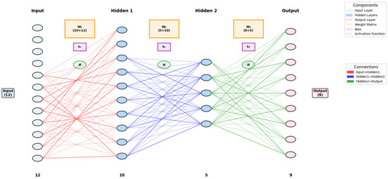
Figure 1.
Error prediction neural network.
The neural network in Figure 1 is configured with only two hidden layers based on the following considerations: A two-layer hidden structure ensures sufficient modeling capability while avoiding an overly complex network architecture. This is particularly suitable for problems like inertial navigation error compensation, which are nonlinear but supported by clear physical models. Theoretically, a network with two hidden layers can approximate most complex nonlinear functions, especially when dealing with attitude, velocity, and position errors in inertial navigation systems, capturing the interactions between different error sources. A two-layer network strikes a balance between training speed and generalization ability, avoiding the risks of overfitting and wasted computational resources due to excessive layers. The setting of the number of nodes in the two hidden layers of the network is based on the following considerations: From the input layer (12 features) to the first hidden layer (10 nodes) to the second hidden layer (5 nodes) and then to the output layer (9 response variables or a single response variable), it reflects the process of information compression and extraction, aligning with the “funnel principle” in neural network design. The first layer with 10 nodes is mainly responsible for extracting basic feature patterns from the original 12-dimensional features, while the second layer with 5 nodes further integrates these features to extract higher-level abstract representations, helping to capture the intrinsic patterns of inertial navigation system errors. The relatively small number of nodes (a total of 15 hidden nodes) helps avoid overly complex networks, especially when using efficient training algorithms such as Bayesian regularization (trainbr) and Levenberg–Marquardt (trainlm), maintaining good generalization ability. In inertial navigation error modeling, the relationship between input data (attitude error, velocity error, etc.) and output has a certain physical significance and correlation, allowing for good fitting results without requiring particularly complex network structures.
Table 1 lists the relevant parameters of the constructed DNN. The numbers of neurons in the input layer, hidden layers, and output layer, as well as the number of hidden layers, are clearly shown in Figure 1, so they are not repeated in the table.

Table 1.
Parameter value or type.
4.2. Network Training and Optimization
This study constructed a complete training dataset based on actual navigation data. The dataset includes angular increments and velocity increments collected by the IMU, as well as attitude and velocity obtained from the SINS as features; with attitude angle errors, velocity errors, and position errors as response variables. The data collection frequency is 100 Hz, and a total of 5 × 10³ s of navigation data were collected, forming 5 × 10⁵ sample points.
To ensure the model’s generalization ability, a standard dataset division strategy was adopted: divided into a training set and test set in a ratio of 7:3. The training set is used for network parameter optimization, and the test set for evaluating the model’s generalization ability. This division method ensures the sufficiency of training data while avoiding the risk of overfitting.
To improve network training efficiency and prediction accuracy, input features and output responses were standardized. The standardization process is based on the statistical characteristics of the training set, calculating the mean and standard deviation of each feature, and then converting all data into a standard normal distribution with a mean of 0 and a standard deviation of 1. This processing helps eliminate the impact of differences in feature dimensions, accelerates network convergence, and improves training stability. Similarly, the response variables were standardized. During the prediction phase, the network output needs to be de-standardized to restore the original dimensions.
Considering the characteristic differences of different types of navigation errors, this study adopted a “one error per network” parallel architecture, training independent neural networks for nine error variables (three attitude angle errors, three velocity errors, three position errors). Each network uses a two-hidden-layer structure, with five neurons in both the first and second hidden layers, and the activation function is ReLU (Rectified Linear Unit). Network training uses the Levenberg–Marquardt (LM) algorithm, which combines the advantages of gradient descent and Gauss–Newton methods, suitable for training small to medium-sized neural networks. The maximum number of training iterations is set to 1000, the target error is set to , and the minimum gradient is set to . These parameter settings ensure sufficient training while avoiding overtraining. To prevent overfitting, this study adopted an early stopping strategy, which terminates the training process early if the performance on the validation set does not improve for 10 consecutive iterations. This method effectively prevents the network from overfitting the training data and improves the model’s generalization ability on unseen data. The model inference time, hardware configuration, and software environment parameters are shown in Table 2.
Table 2.
Model inference-related parameters.
During training, the system automatically records the performance on the validation set after each training iteration and saves the network parameters with optimal performance, ensuring the final model has the best generalization ability. After training is completed, the network performance is comprehensively evaluated using the test set, with mean squared error as the evaluation metric. The specific performance is shown in Figure 2 and Table 3. In addition, we also included the most commonly used time series prediction method—LSTM for comparison. Unlike the DNN, the input and output of the LSTM are both the error states, namely the attitude, velocity, and position errors. In other words, both the features and responses are 9-dimensional vectors.
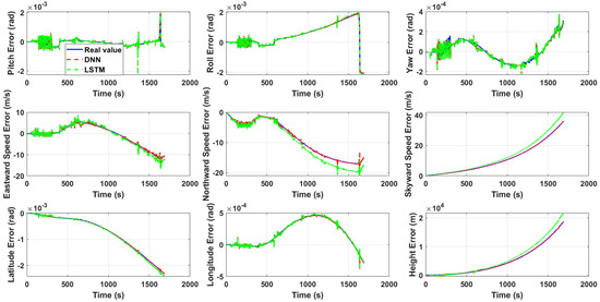
Figure 2.
Test set neural network output.
Table 3.
MSE of response variables for test set.
In Figure 2, the true values (i.e., true errors) are the differences between the attitude, velocity, and position obtained from pure inertial navigation calculations and those obtained from SINS/GPS integrated navigation. In other words, the results of SINS/GPS integrated navigation are regarded as the true state, while the results of pure inertial navigation calculations are regarded as the observed state. The difference between the two is the true error, which is used to learn the nonlinear patterns of errors with a DNN, allowing for prediction and compensation when GPS signals are unavailable.
The test set performance comparison between DNN and LSTM models reveals that the DNN achieves exceptionally high prediction accuracy, with errors for each response variable typically on the order of 10−5 or lower. These results demonstrate both the strong generalization capability of the proposed network architecture and the feasibility of employing DNN for inertial navigation system error prediction. In contrast, the LSTM model maintains reasonable prediction accuracy during the initial phase but progressively deviates from the true error values after 500 s. As shown in Table 3, the MSE values for multiple response variables predicted by the LSTM are orders of magnitude higher than those achieved by the DNN. The inferior performance of LSTM in SINS error prediction can be attributed not only to the factors discussed in Section 4.1, but also potentially to the hyperparameter settings, particularly the time step configuration, which was set to 200 in this study.
5. Experimental Results and Performance Analysis
Using the same set of IMU from chapter 3, the FOG (Fiber Optic Gyroscope) inertial measurement unit (specific information can be found in Figure 3 and Table 4 and Table 5) using IMU-ISA-100C has a sampling frequency of 100 Hz; GPS uses a differential mode with an output frequency of 10 Hz. It first remained stationary for 690 s for self-alignment, then moved with a vehicle outdoors in Xi’an city for approximately 3 h; the slow speed is about 3.5 m/s and the driving range is within 10 km; the equipment layout in the vehicle is shown in Figure 4. The outputs of the gyroscope and accelerometer are shown in Figure 5. Firstly, the SINS/GPS integrated navigation system was used for calculation, and the results were taken as the true values. The attitude, velocity, and position obtained from the SINS, as well as the attitude, velocity, and position predicted and corrected by the DNN trained in Section 4.1, were compared with the true values. Meanwhile, to highlight the predictive advantages of DNN in multi-dimensional features and multi-dimensional responses, we also included the attitude, velocity, and position predicted and corrected by LSTM in the comparison. In other words, the attitude, velocity, and position of the integrated navigation system are the true values, while the attitude, velocity, and position calculated by the SINS, the attitude, velocity, and position predicted and corrected by DNN, and the attitude, velocity, and position predicted and corrected by LSTM are the comparison values. The curves were plotted using Matlab to simulate the actual motion state of the carrier. The comparisons of attitude, velocity, and position are shown in Figure 6, Figure 7, Figure 8 and Figure 9. To more clearly distinguish the accuracy of different methods, the error curves of attitude, velocity, and position are also plotted, as shown in Figure 10. Table 6 lists the MSE of navigation errors for different methods.
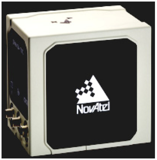
Figure 3.
Inertial measurement unit.
Table 4.
Gyroscope parameters.
Table 5.
Accelerometer parameters.
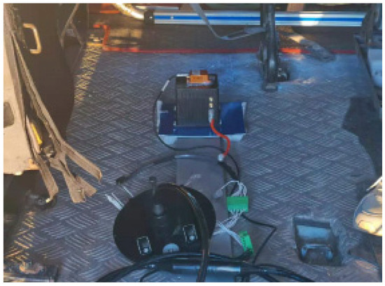
Figure 4.
Equipment layout.
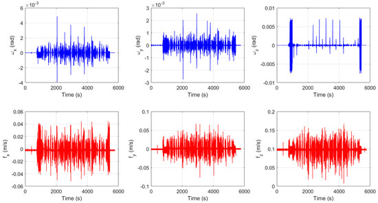
Figure 5.
The outputs of the gyroscope and accelerometer.
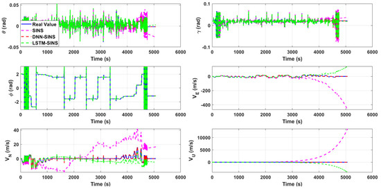
Figure 6.
Comparison of attitude and velocity.
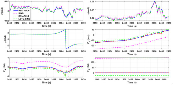
Figure 7.
Attitude and velocity comparison (partial enlargement).
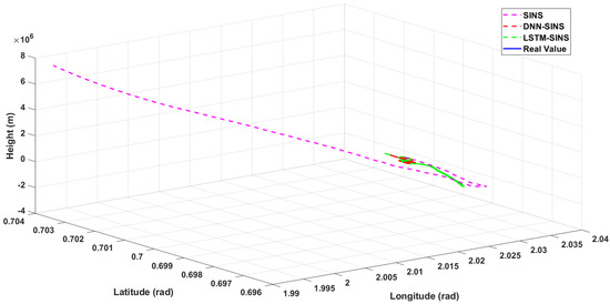
Figure 8.
Three-dimensional position comparison.
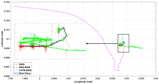
Figure 9.
Plane position comparison.
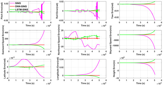
Figure 10.
Error comparison.
Table 6.
MSE of navigation errors for different methods.
Figure 6 and Figure 7 show the comparison of attitude and velocity for the three methods, with a zoomed-in section of approximately 20 s of data. In Figure 6, due to the high accuracy of the IMU used in the experiment and the relatively short sampling time, the differences in attitude among the four methods are not very pronounced, although the attitudes predicted and corrected by DNN and LSTM are obviously closer to the true values than SINS. However, in Figure 7, there are still significant gaps in velocity and position accuracy among the three methods. It can be intuitively observed that the attitude, velocity, and position calculated by SINS have considerable deviations from the true values, with the skyward velocity showing a deviation of hundreds of meters per second. The values predicted and compensated by DNN and LSTM show significantly reduced deviations from the true values, but intuitively, the deviation of DNN from the true values is obviously smaller than that of LSTM. In Figure 8, the three-dimensional trajectory calculated by SINS only coincides with the real trajectory in the initial stage of carrier movement, after which the deviation gradually increases and is particularly pronounced in height performance. After error prediction and correction using DNN and LSTM, the height is essentially at the same level as the real height. For ground-moving carriers, the planar position is of greater concern to us. In Figure 9, the two-dimensional trajectory clearly shows that the planar trajectory predicted and corrected by DNN basically fluctuates around the real trajectory. LSTM prediction also shows a certain effectiveness, but its fluctuation is more pronounced, and the movement direction in the later stage is opposite to the carrier’s true movement direction. In contrast, the planar trajectory calculated by SINS basically cannot describe the carrier’s true movement.
Figure 6, Figure 7, Figure 8 and Figure 9 can only provide qualitative judgment of the differences between different methods, while Figure 10 allows for quantitative analysis of the accuracy of each method. In terms of pitch error, the maximum value of SINS calculation is 2.5 × 10⁻² radians, SINS-LSTM is 3.3 × 10⁻³ radians, and SINS-DNN is 1.07 × 10⁻³ radians. For roll error, the maximum value of SINS calculation is 2.0 × 10⁻² radians, SINS-LSTM is 3.14 × 10⁻³ radians, and SINS-DNN is 4.70 × 10⁻⁴ radians. In terms of yaw error, the maximum value of SINS calculation is 2.42 × 10⁻² radians, SINS-LSTM is 3.86 × 10⁻³ radians, and SINS-DNN is 1.10 × 10⁻⁴ radians. For eastward velocity error, the maximum value of SINS calculation is 455 m/s, SINS-LSTM is 135 m/s, and SINS-DNN is 4.71 m/s. For northward velocity error, the maximum value of SINS calculation is 26.8 m/s, SINS-LSTM is 8.22 m/s, and SINS-DNN is 4.16 m/s. In terms of skyward velocity error, the maximum value of SINS calculation is 1.34 × 10⁴ m/s, SINS-LSTM is 3.74 × 10³ m/s, while SINS-DNN remains stable within 10 m/s. For latitude error, the maximum value of SINS calculation is 3.83 × 10⁻³ radians, SINS-LSTM is 9.68 × 10⁻⁴ radians, and SINS-DNN is 7.45 × 10⁻⁴ radians. In terms of longitude error, the maximum value of SINS calculation is 3.82 × 10⁻² radians, SINS-LSTM is 5.97 × 10⁻³ radians, and SINS-DNN is 1.5 × 10⁻⁴ radians. For height error, the maximum value of SINS calculation is 7.7 × 10⁶ m, SINS-LSTM is 2.2 × 10⁶ m, while SINS-DNN remains within 10 m. From the above analysis, it can be seen that overall, regardless of which method is used for prediction and correction, the accuracy is higher than pure inertial navigation calculation, with attitude, velocity, and position errors all significantly reduced. For carriers with planar motion, heading and position accuracy are of primary concern. Therefore, examining the errors in yaw and latitude/longitude, between SINS-LSTM and SINS-DNN, except for the relatively close latitude error, all other errors differ by an order of magnitude. This leads to the fact that in Figure 8, the motion trajectory of SINS-DNN is more closely aligned with the real trajectory than SINS-LSTM, in other words, SINS-DNN has a higher positioning accuracy.
In terms of height, it is evident from the experimental results that both DNN and LSTM significantly reduce the height error. The underlying reason is that pure inertial navigation tends to diverge rapidly in the height channel, while prediction and compensation using DNN or LSTM essentially introduce height damping, resulting in an immediate improvement. However, for ground or surface vehicles, the height value is not a primary navigation parameter of interest. Therefore, although the error is significantly reduced, we do not discuss it in detail.
6. Conclusions and Prospects
This study proposes a DNN-based method for predicting and correcting the errors of SINS, aiming to address the persistent challenge of long-term error accumulation in inertial navigation. By constructing a prediction model that takes angular and velocity increments, as well as real-time attitude and velocity states as input features, and by using attitude, velocity, and position errors as multidimensional response targets, the method effectively captures the nonlinear, integrated propagation mechanisms of inertial errors. Experimental results based on both simulation and real-world vehicle motion data demonstrate that the proposed DNN approach significantly outperforms traditional SINS- and LSTM-based predictions in terms of accuracy and stability, particularly in maintaining position and heading consistency over extended durations. The method shows robust adaptability in GPS-denied environments, offering a promising alternative or complement to integrated navigation systems dependent on external signals. Nevertheless, the current model’s effectiveness is closely tied to the characteristics of the inertial hardware used during training, which may limit its generalization across different IMU devices. Future research will focus on enhancing cross-device generalization through transfer learning and domain adaptation techniques, as well as exploring lightweight network architectures for real-time onboard deployment in constrained platforms such as UAVs and underwater vehicles.
Of course, this study also has some unresolved issues at present. Among them, a key issue is that the navigation errors predicted using DNN or LSTM in the study represent the total sum of errors including the effects of inertial device errors, temperature errors, as well as vehicle maneuvering and environmental factors. In other words, the study does not involve the estimation and compensation of various types of errors. Therefore, the methods involved in this study would theoretically only have significant effects when using the same IMU, in roughly the same external environment, and when vehicle maneuvering changes are not drastic. This also limits the universality of the method to some extent. However, this does not mean that the research content and results are worthless. In the future, it might be possible to consider incorporating factors such as temperature into the features, implementing adaptive error learning for spatial environment and temperature using multi-layer recurrent neural networks [17,18] composed of LSTM and RNN.
Author Contributions
J.L. was responsible for manuscript writing in this study, T.Z. was responsible for project management and supervision, L.C. undertook funding acquisition, and P.L. was responsible for data analysis. All authors have read and agreed to the published version of the manuscript.
Funding
This work was supported by the National Natural Science Foundation of China (62373367).
Data Availability Statement
In accordance with relevant university regulations, the raw data and programs involved in this study cannot be fully disclosed at present. If there is a genuine need for academic research and communication, please contact the corresponding author (ztr0820@whu.edu.cn) for discussion. However, disclosure without the author’s permission is not permitted.
Conflicts of Interest
The author declares that there are no financial or personal relationships that could have inappropriately influenced the work reported in this thesis. No conflicts of interest exist in relation to this research.
References
- Zhao, H.; Xiong, Z.; Yu, F.; Pan, J.; Sun, Y. An integrated navigation algorithm for Aerospace Vehicle based on extended H ∞ filter. In Proceedings of the 33rd Chinese Control Conference, CCC, Nanjing, China, 28–30 July 2014; pp. 822–826. [Google Scholar]
- Zhang, Z.Y.; Li, Y.; Wang, J.Y.; Liu, Z.; Jiang, G.; Guo, H.; Zhu, W. A hybrid data-driven and learning-based method for denoising low-cost IMU to enhance ship navigation reliability. Ocean Eng. 2024, 299, 117280. [Google Scholar] [CrossRef]
- Skog, I.; Händel, P. In-Car Positioning and Navigation Technologies—A Survey. Intelligent Transportation Systems. IEEE Trans. Intell. Transp. Syst. 2009, 10, 4–21. [Google Scholar] [CrossRef]
- Shen, C.; Zhang, Y.; Tang, J.; Cao, H.; Liu, J. Dual-optimization for a MEMS-INS/GPS system during GPS outages based on the cubature Kalman filter and neural networks. Mech. Syst. Signal Process. 2019, 133, 106222. [Google Scholar] [CrossRef]
- Nourmohammadi, H.; Keighobadi, J. Design and experimental evaluation of indirect centralized and direct decentralized integration scheme for low-cost INS/GNSS system. GPS Solut. 2018, 22, 1–18. [Google Scholar] [CrossRef]
- Yao, Y.Q.; Xu, X.S.; Li, Y.; Zhang, T. A Hybrid IMM Based INS/DVL Integration Solution for Underwater Vehicles. IEEE Trans. Veh. Technol. 2019, 68, 5459–5470. [Google Scholar] [CrossRef]
- Chang, L. Multiplicative extended Kalman filter ignoring initial conditions for attitude estimation using vector observations. J. Navig. 2023, 76, 62–76. [Google Scholar] [CrossRef]
- Alawieh, H.; Sahili, J. A Cascaded kalman filter model-aided inertial navigation system for underwater vehicle. In Proceedings of the2019 7th International Conference on Robotics and Mechatronics (ICRoM), Tehran, Iran, 20–21 November 2019; pp. 104–109. [Google Scholar]
- Shafay, M.; Ahmad, R.W.; Salah, K.; Yaqoob, I.; Jayaraman, R.; Omar, M. Blockchain for deep learning: Review and open challenges. Clust. Comput. 2023, 26, 197–221. [Google Scholar] [CrossRef] [PubMed]
- Ghadarjani, R.; Gharaei, N.K. Implanting deep learning models for burn wound assessment. Burns 2024, 50, 286–287. [Google Scholar] [CrossRef] [PubMed]
- Suh, D.; Lee, J.W.; Choi, S.; Lee, Y. Recent Applications of Deep Learning Methods on Evolution- and Contact-Based Protein Structure Prediction. Int. J. Mol. Sci. 2021, 22, 6032. [Google Scholar] [CrossRef] [PubMed]
- He, Q.Y.; Yu, H.P.; Fang, Y.C. Deep Learning-Based Inertial Navigation Technology for Autonomous Underwater Vehicle Long-Distance Navigation—A Review. Gyroscopy Navig. 2023, 14, 267–275. [Google Scholar]
- Jiang, C.; Chen, Y.; Chen, S.; Bo, Y.; Li, W.; Tian, W.; Guo, J. A Mixed Deep Recurrent Neural Network for MEMS Gyroscope Noise Suppressing. Electronics 2019, 8, 181. [Google Scholar] [CrossRef]
- Wu, F. Optimizing GNSS/INS Integrated Navigation: A Deep Learning Approach for Error Compensation. IEEE Signal Process. Lett. 2024, 31, 3104–3108. [Google Scholar] [CrossRef]
- Liu, Y.; Luo, Q.; Zhou, Y. Deep Learning-Enabled Fusion to Bridge GPS Outages for INS/GPS Integrated Navigation. IEEE Sens. J. 2022, 22, 8974–8985. [Google Scholar] [CrossRef]
- Ma, L.H.; Li, Q.; Chen, Y.F.; Luo, X.; Kai, L.; Zhang, S. Installation angle calibration between the star sensor and gyro unit using the equivalent rotation vector transformation. Meas. Sci. Technol. 2024, 35, 065010. [Google Scholar] [CrossRef]
- Su, H.; Schmirander, Y.; Li, Z.; Zhou, X.; Ferrigno, G.; De Momi, E. Bilateral Teleoperation Control of a Redundant Manipulator with an RCM Kinematic Constraint. In Proceedings of the IEEE International Conference on Robotics and Automation (ICRA), Paris, France, 31 May–31 August 2020; pp. 4477–4482. [Google Scholar]
- Wen, Q.; Ovur, S.E.; Li, Z.; Marzullo, A.; Song, R. Multi-Sensor Guided Hand Gesture Recognition for a Teleoperated Robot Using a Recurrent Neural Network. IEEE Robot. Autom. Lett. 2021, 6, 6039–6045. [Google Scholar]
Disclaimer/Publisher’s Note: The statements, opinions and data contained in all publications are solely those of the individual author(s) and contributor(s) and not of MDPI and/or the editor(s). MDPI and/or the editor(s) disclaim responsibility for any injury to people or property resulting from any ideas, methods, instructions or products referred to in the content. |
© 2025 by the authors. Licensee MDPI, Basel, Switzerland. This article is an open access article distributed under the terms and conditions of the Creative Commons Attribution (CC BY) license (https://creativecommons.org/licenses/by/4.0/).