Three-Dimensional Phase-Space Design and Simulation of a Broadband THz Transmission Line Using Wigner Optics and Ray Tracing

Abstract

Designing a transmission line (TL) for a widely tunable, broadband terahertz radiation source presents substantial challenges due to the complexity of beam dynamics and spectral characteristics. Here, we investigate the propagation of the most significant radiation modes expected to traverse the TL, intended for integration with an advanced particle accelerator currently under construction at the Schlesinger Family Center for Compact Accelerators, Radiation Sources and Applications. The total electromagnetic field at the source output is expressed in the frequency domain via cavity eigenmodes and transformed into an optical field representation using the Wigner distribution function (WDF). This formulation enables physically consistent modeling within the constraints of geometric optics and Wigner formalism of the spatiotemporal evolution of the radiation during propagation. The initial TL design is developed and optimized based on this representation. A 3D space–frequency analysis tool for pulsed radiation, based on the WDF, was implemented to characterize field behavior and guide system development. Complementary ray tracing simulations were conducted using the Zemax Optic Studio platform, supporting the assessment of optical feasibility through simulation and system feasibility.

1. Introduction

1.1. Purpose and General Representation

Recent years have seen significant advances in the study of terahertz (THz) radiation. This spectral range (0.3–3.75 THz) is non-ionizing and therefore considered safe for biological systems [1,2], yet it possesses the ability to penetrate a variety of non-conductive materials such as plastic, cotton, and even certain layers of human skin. These unique characteristics have led to a surge of interest across multiple scientific disciplines, especially in biomedical applications [3]. In medicine, for instance, THz-based imaging techniques have been developed for early cancer detection [4,5], while in security, THz imaging [6] is employed for the detection of concealed weapons. More broadly, THz waves enable non-destructive inspection of hidden internal substances, paving the way for novel techniques in material analysis. As a result, THz research and applications have become increasingly popular and accessible [7,8].

In response to the growing demand for high-intensity THz sources, the Schlesinger Family Center for Compact Accelerators, Radiation Sources & Applications at Ariel University has initiated the development of a dedicated Free Electron Laser (THz-FEL) system [9]. However, the propagation of THz radiation remains a challenging problem, as it exhibits both optical and electromagnetic (EM) wave characteristics [10]. Accurately modeling THz signal transmission from a source thus involves significant complexity. Although the transfer matrix method [11] has shown progress in recent THz applications, traditional EM modeling techniques remain inadequate for generalized solutions, especially for the transmission line (TL) design for a wide tunable broad-spectrum THz radiation source [10]. In the design of the TL, waveguide, or 3D printed mirror surface (antenna, e.g., cast coatings) [12], various mechanical parameters must be considered, as they influence the behavior of the incident pulses. These include effects such as creeping waves [13] caused by surface imperfections in the waveguide walls [14] or the intrinsic material properties of the TL components. This study relies on a previously established model at the waveguide exit, assuming that such effects are already incorporated into the electromagnetic field description and subsequently translated into ray-based propagation methods.

This work focuses on the complexity of beam dynamics and spectral dispersion in a broadband THz FEL system [9] for the design and simulation of a quasi-optical TL that will guide the THz beam from the FEL to a user facility located approximately 10 m from the source. Effective TL design requires a thorough characterization of the EM field along the beam path (or TL). Historically, THz beam analysis has been predominantly physical in nature—that is, problem definitions were based on physical intuition and addressed analytically. Commercial software tools such as CST have proven insufficient for this task, largely due to the difficulty in defining specific boundary conditions and the complexity of the field distributions. Numerical methods are therefore essential, although these too often lack generality and broad applicability [10]. Electromagnetic solvers and algorithms—such as FDTD—typically demand a minimum of 10 spatial samples per wavelength in each dimension. Consequently, the spatial mesh-cell size (Δr) must be on the order of 10 µm. The temporal step size (Δt) is intrinsically linked to the spatial resolution, governed by the relation Δr ≫ c₀Δt, where c₀ denotes the speed of light in vacuum. Based on these constraints, solving the problem would necessitate approximately 10¹⁷ spatial mesh points and around 10⁶ time steps [10].

In this study, we present a comprehensive characterization of THz radiation, particularly in the context of ultra-narrow pulses spanning a broad frequency spectrum. The analysis is aimed at informing the design of the quasi-optical TL required to efficiently transport this complex EM field. The ultimate goal is to achieve maximal energy transfer efficiency through precise modeling of the TL.

An approximate model of the EM beams was first obtained through experimental studies involving an undulator (wiggler). Building upon this, we implemented simulations based on the Wigner distribution function (WDF) [10,15], combining both analytical and numerical methods [16]. The WDF enables a phase-space representation of the EM field in terms of geometrical optics (GO) rays, which can be computed using standard GO rules. This duality significantly simplifies complex field calculations while maintaining accuracy, especially when combined with transfer matrix formalism tailored to specific user requirements.

We introduced a general tool for computing 3D THz beam propagation, utilizing the WDF in combination with ray tracing (RT) methods via the Zemax Optic Studio software (version 13). The primary focus was on the space–frequency representation of the EM field, providing both insight and design parameters. Notably, the contribution of each mode is evaluated individually to assess the TL’s response. This enables estimation of how future TL parameters should be adapted in response to changes in the undulator’s waveguide configuration.

In previous work [10], the EM field analysis was performed using a simplified model involving a flat aperture (7.5 × 5 mm) in place of a waveguide. In contrast, the present study calculates individual mode contributions analytically, using a real waveguide sourced from a commercial catalog, thereby achieving significantly higher accuracy.

The THz-FEL source is driven by a photo-injector RF LINAC gun that produces femtosecond-scale electron bunches. This RF LINAC employs a hybrid structure composed of both standing-wave and traveling-wave sections, yielding broadband electron beams with controlled energy chirps. THz radiation is emitted from a 12 × 6 mm flat aperture, the output of the waveguide (undulator/wiggler), with a spectral bandwidth of approximately 10% around the central resonance frequency. The system offers tunability in the 1–3.5 THz range, with the resulting EM field energy distributed across three distinct waveguide modes [17]. The modal structure in the frequency domain is derived from a space–frequency formulation of ultrawideband interactions in free-electron lasers [18], and it incorporates enhancements from coherent spontaneous emission FELs and prebatched FEL configurations that employ periodically modulated short electron beam pulses [17]. The general layout of the THz FEL is depicted in Figure 1.

1.2. Review of Simulation Methods

Numerous methods exist for calculating EM radiation transmission, spanning both classical and contemporary approaches, and encompassing both analytical and numerical techniques [19]. The present study adopts a hybrid approach, wherein the EM field is transformed into a GO ray set (representation using the WDF). This formulation facilitates integration with the RT technique, which is implemented using the Zemax Optic Studio software—purpose-built for such optical modeling.

Alternative simulation approaches were evaluated but ultimately excluded due to inconsistencies and limitations, as detailed in a prior study [10], thereby obviating the need for extensive discussion here. As previously noted, Zemax is employed in this work to perform high-precision RT simulations, essential for accurate analysis of the radiation’s optical path (or TL).

It is also worth emphasizing that RT is not limited to applications in computer graphics or conventional optical systems; it has been widely adopted in the analysis of EM propagation, including in the millimeter-wave [20] and radio-frequency domains [21]. Given its proven utility in those contexts, its applicability to THz radiation is both reasonable and promising.

1.3. The Main Goal

The simulation developed in this work is intended to support the future design of the TL, with the aim of accurately modeling the propagation of EM fields along the designated optical trajectory. Ultimately, the divergence and spatial distribution of the beams will define focal positions, beam diameters, and optical path lengths.

The radiation emitted from the source will be delivered to the user room via the TL, operating under vacuum conditions. The TL comprises a set of four confocal off-axis parabolic mirrors housed within a 30 cm diameter TL (or beamline), as illustrated in Figure 2. In accordance with classical optical design principles, the initial configuration of the TL is proposed to include a first mirror pair with focal lengths F₁/F₂ = 200/450 mm, followed by a second pair with focal lengths F₃/F₄ = 1550/350 mm.

2. Materials and Methods

2.1. WDF—Wigner Methodology

The WDF, introduced by E. Wigner [22], represents the simplest quantum analogue of the classical phase-space distribution function, enabling the computation of probabilities and expectation values of quantum operators in a form that closely mirrors the classical method. In optics, WDF was first applied over three decades ago [23], and it has since become a powerful tool in various domains.

Today, WDF enjoys widespread application in the theoretical analysis of optical systems—including quasi-optical configurations [24]—as well as in acoustics [25], signal processing [26], wireless communication via radio waves [27], and radar emitter characterization [28]. A majority of studies focus on one-dimensional time-frequency analysis using the WDF framework [29]. However, the present work emphasizes a more general, three-dimensional spatial-frequency approach to EM field analysis, particularly where classical ray descriptions fall short in capturing the complexity of free-space EM wave propagation [30].

While the use of WDF in THz radiation systems has been reported [31], the methodology is general and can be applied to a broad class of radiative systems. Of particular interest is the imaging of partially coherent optical beams and the comprehensive modeling of EM field evolution during propagation. This is achieved via phase-space representations such as mutual intensity (MI), which describe a stochastic field in either the spatial or spatial-frequency domain [32].

The MI characterizes beam evolution through the correlation function.

$\Gamma \left({\mathit{r}}_1,{\mathit{r}}_2\right)=\langle f\left({\mathit{r}}_1\right)f$*$\left({\mathit{r}}_2\right)\rangle$, which depends on two position vectors, r₁ and r₂. Here, $f$*$\left({\mathit{r}}_2\right)$ denotes the complex conjugate of the field, and the angle brackets represent spatial or temporal averaging. For clarity, we refer to this formulation as the Modified Correlation Function (MCF), capturing the coherence between field oscillations at two spatial locations.

The intensity distribution I(r) can be obtained as the diagonal component of the MI:

$$\Gamma \left(r,r\right)=\langle |{f\left(r\right)|}^2\rangle .$$

The Wigner distribution of the EM field, W(r,p), is then defined via the MCF, or alternatively, in terms of the field’s directional spectrum [32,33]. This formulation provides a rich representation of both spatial and angular (momentum) information, thereby facilitating precise modeling of beam propagation in complex THz transmission systems.

$$W(r,p)=\int \Gamma (r+{\displaystyle \frac{\tilde{r}}{2}},r-{\displaystyle \frac{\tilde{r}}{2}})e^{\left(-i2\pi p\tilde{r}\right)}d\tilde{r}$$

(1)

$$W\left(r,p\right)=\int \overline{\Gamma }(p+{\displaystyle \frac{\tilde{p}}{2}},p-{\displaystyle \frac{\tilde{p}}{2}})e^{\left(+i2\pi r\tilde{p}\right)}d\tilde{p}$$

(2)

2.2. Light Field or Ray Concept

It is evident that the space–frequency description corresponds directly to the Light Field (LF) theory [34], where each ray can be characterized by its passage through a point r with a spatial frequency p (i.e., direction q). Let us define a “Ray Concept” whereby each ray is described by its spatial position and direction and is associated with an amplitude W(r,p), which in our context is complex-valued.

In accordance with the LF theory [34], computational imaging principles [35], and the general ray concept [36], EM field propagation from a source point in space can be described using a set of GO rays, derived through the WDF. Below, a 2D scenario is considered, where the EM field propagates in a plane perpendicular to the Z axis within a waveguide. Note that upon exiting the waveguide, the beams expand and propagate in three dimensions. We define a simple monochromatic field distribution at the waveguide output (the aperture), and the WDF is expressed as

$$W_{\left\{x,y\right\}}{\left.\left(x,y,k_x,k_y\right)\right|}_{z_{aperture}}=\iint \left(MCF\right){·e}^{\left(+i{k}_x\tilde{x}\right)}·e^{\left(-i{k}_y\tilde{y}\right)}d\tilde{x}d\tilde{y}$$

(3)

where

$$MCF=E_{\{x,y\}}^{\ast }{\left.\left(x-{\displaystyle \frac{\tilde{x}}{2}},y-{\displaystyle \frac{\tilde{y}}{2}}\right)\right|}_{z_{aperture}}{·E}_{\{x,y\}}{\left.\left(x+{\displaystyle \frac{\tilde{x}}{2}},y+{\displaystyle \frac{\tilde{y}}{2}}\right)\right|}_{z_{aperture}}$$

(4)

Here, $W_{\{x,y\}}$ represents the WDF of the electric field $E_{\{x,y\}}$, with x and y being coordinates on the aperture surface, and $k_x,k_y$ being the Fourier conjugates to these spatial coordinates. By introducing time dependence into the beam transfer process, the WDF’s dimensionality increases from 4D to 6D.

The resulting LF comprises rays emanating from each point (x, y) on the aperture. The wave (number) vector $\mathit{k}={(k}_x,k_y,k_z)$ specifies the 3D direction of each ray, with the third component of propagation in the free space, defined as

$$k_z=\sqrt{{\left({\displaystyle \frac{\omega }{c}}\right)}^2-k_x^2-k_y^2}$$

(5)

Alternatively, the WDF can be expressed in terms of spatial frequency components:

$$k_x={\displaystyle \frac{2\pi }{\lambda }}\cos {\theta }_x\hspace{1em}\hspace{1em}\hspace{1em}{k}_y={\displaystyle \frac{2\pi }{\lambda }} \cos {\theta }_y$$

(6)

where $\cos {\theta }_x$ and $\cos {\theta }_y$ are the projections of the wave front onto the X and Y axes, respectively (angles θ_x and θ_y represent the projections of the wave vector components with respect to the transverse axes, the Z axis, consistent with the 3D wavevector).

The magnitude and polarization of each ray are defined via the WDF as follows:

$$I_x(x,y,k_x,k_y)=W_x(x,y,k_x,k_y)\hspace{1em}{I}_y(x,y,k_x,k_y)=W_y(x,y,k_x,k_y)$$

(7)

Due to the orthogonality condition in uniform media between the ray’s polarization and its wavevector (i.e., $\mathit{I}\perp \mathit{k}$), the z-component of the polarization is given by

$$I_z=\left\{\begin{array}{c}-{\displaystyle \frac{I_x·k_x+I_y·k_y}{k_z}} k_z\ne 0\\ 0 k_z=0\end{array}\right.$$

(8)

Therefore, the LF is effectively described as the GO ray set, each uniquely defined by its initial position (x, y) at the aperture, the field amplitude I$(x,y,k_x,k_y$), and its directional vector ${(k}_x,k_y,k_z)$. The propagation of any signal through space then adheres to the rules of GO ray theory [33].

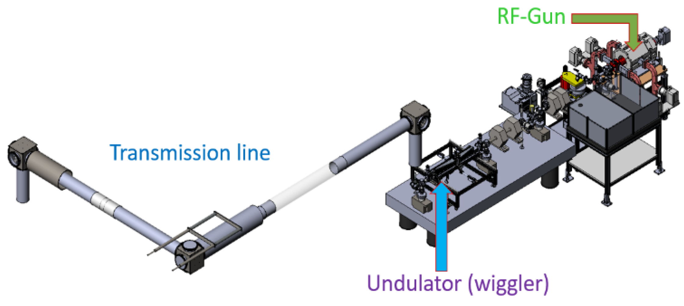
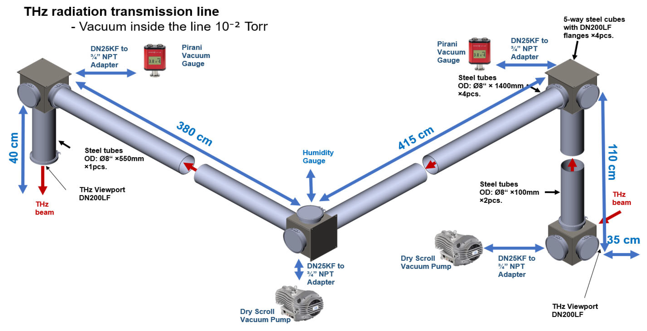
2.3. Simulation Preparation: System Planning and Construction

To perform the radiation transfer simulations, Matlab files must be prepared in a format compatible with the Zemax simulator. Concurrently, a model of the TL was developed, based on a previously simplified and optimized version. This included, for example, replacing mirrors with equivalent thin lens models, aligning the system, and simplifying the common transfer matrix for confocal mirrors. The comprehensive design and optimization of the transmission line (TL)—including the selection of construction materials, vacuum level, associated pumping systems, mirror coatings, and related components—are beyond the scope of the present study.

The simulation method proposed here for THz beam propagation represents a compromise between linear optics and full analytical solutions of Maxwell’s equations. While linear optics offers simplicity, it lacks the accuracy required to capture spatial beam evolution at THz frequencies. On the other hand, solving Maxwell’s equations analytically is often complex and computationally intensive.

Our approach employs the WDF, transitioning from a continuous field distribution to a discrete set of rays that can be treated within classical optics. This technique is specifically adapted for the THz frequency domain. Initially, the electric field’s WDF is computed analytically. A ray array is then generated, with each ray defined by a specific position, angle, and intensity according to the WDF. These rays are propagated through the optical system, and the WDF is reconstructed at the output. If necessary, the EM field can be recovered from the WDF. However, since the WDF is not a dual function, its inverse transformation is nontrivial.

Several approximation methods exist for reconstructing the EM field, though some may introduce singularities at the origin. For the purposes of this study—and potentially for future TL designs—EM field reconstruction is not required. In fact, characterizing the EM field using GO rays (or LF) representations is often more practical, especially when using the Zemax simulator.

The algorithm is capable of simulating any TEmn or TMmn mode. However, this study focuses on three dominant modes in the FEL system: TE_01x, TE_21x, and TE_23x (as illustrated in Figure 3). These modes contribute significantly to the total energy—approximately 33% for TE₀₁, 22% for TE₂₁, and 30% for TE₂₃ [37]—as also depicted in Figure 3.

2.4. Analytical Calculation of the WDF

We focus on the transverse distribution of the electric field within the waveguide, perpendicular to the beam’s direction of propagation. Specifically, we consider the spatial components of the electric field (E-field) in the TE mode [3], described as follows:

$${\mathrm{E}}_x\left(x,y\right)=A_{mn}{\displaystyle \frac{-i{2\pi c\mu }_0{k}_{o_y}}{k_{⏊}^2\lambda }}\mathit{cos}\left(k_{o_x}x\right)\mathit{sin}\left(k_{o_y}y\right)$$

(9)

$${\mathrm{E}}_y\left(x,y\right)=A_{mn}{\displaystyle \frac{-i{2\pi c\mu }_0{k}_{o_x}}{k_{⏊}^2\lambda }}\mathit{sin}\left(k_{o_x}x\right)\mathit{cos}\left(k_{o_y}y\right)$$

(10)

The field modes are defined within the spatial bounds X ∈ [0, a] and Y ∈ [0, b] where

• λ: Beam wavelength;
• $A_{mn}:\mathrm{T}\mathrm{h}\mathrm{e} \mathrm{a}\mathrm{m}\mathrm{p}\mathrm{l}\mathrm{i}\mathrm{t}\mathrm{u}\mathrm{d}\mathrm{e} \mathrm{o}\mathrm{f} \mathrm{t}\mathrm{h}\mathrm{e}{ TE}_{mn} \mathrm{m}\mathrm{o}\mathrm{d}\mathrm{e}$;
• c: Speed of light in vacuum;
• μ₀: Permeability of free space;
• a, b: Waveguide dimensions;
• m, n: Mode indices (numbers).

The transverse wave number k⊥ (transverse wavevector component) is given by

$$k_{⏊}^2={k_{o_x}}^2+{k_{o_y}}^2\hspace{1em}\hspace{1em}\hspace{1em}{k}_o\equiv {\displaystyle \frac{2\pi }{\lambda }}$$

(11)

$$k_{o_x}={\displaystyle \frac{m\pi }{a}} k_{o_y}={\displaystyle \frac{n\pi }{b}}\hspace{1em}\hspace{1em}\hspace{1em}\hspace{1em}\hspace{1em}{k}_{o_z}=\sqrt{{\left({\displaystyle \frac{2\pi }{\lambda }}\right)}^2-k_{⏊}^2}$$

(12)

We shift the coordinate system to center it around zero, i.e., X ∈ [−a/2, a/2] and Y ∈ [−b/2, b/2], allowing the EM field to be redefined over this symmetric range. This translation ensures the WDF is computed in the original domain of X ∈ [0, a] and y ∈ [0, b], while retaining flexibility in axis placement.

As a result, the integration limits for the WDF are bound as follows:

• For the X axis:

$$\left\{\begin{array}{c}-{\displaystyle \frac{a}{2}}<x-{\displaystyle \frac{\tilde{x}}{2}}<{\displaystyle \frac{a}{2}}\\ -{\displaystyle \frac{a}{2}}<x+{\displaystyle \frac{\tilde{x}}{2}}<{\displaystyle \frac{a}{2}}\end{array}\right. \to -2\left({\displaystyle \frac{a}{2}}-\left|x\right|\right)<\tilde{x}<2\left({\displaystyle \frac{a}{2}}-\left|x\right|\right)$$

(13)

• For the Y axis:

$$-2\left({\displaystyle \frac{b}{2}}-\left|y\right|\right)<\tilde{y}<2\left({\displaystyle \frac{b}{2}}-\left|y\right|\right)$$

(14)

Substituting the expressions and solving analytically (focusing on the xx-component of the E-field), the WDF becomes

$$\begin{gathered} W_x\left(x,y,k_x,k_y\right)=\underset{-2\left({\displaystyle \frac{a}{2}}-\left|x\right|\right)}{\overset{2\left({\displaystyle \frac{a}{2}}-\left|x\right|\right)}{\int }}\underset{-2\left({\displaystyle \frac{b}{2}}-\left|y\right|\right)}{\overset{2\left({\displaystyle \frac{b}{2}}-\left|y\right|\right)}{\int }}{E}_x\left(\left(x+{\displaystyle \frac{a}{2}}\right)-{\displaystyle \frac{\tilde{x}}{2}},\left(y+{\displaystyle \frac{b}{2}}\right)-{\displaystyle \frac{\tilde{y}}{2}}\right){E_x}^{\ast }\left(\left(x+{\displaystyle \frac{a}{2}}\right) \\ +{\displaystyle \frac{\tilde{x}}{2}},\left(y+{\displaystyle \frac{b}{2}}\right)+{\displaystyle \frac{\tilde{y}}{2}}\right)e^{-i\left(k_x\tilde{x}+k_y\tilde{y}\right)}d\tilde{y}d\tilde{x} \end{gathered}$$

(15)

This expression can be separated into two independent integrals, yielding

$$W_x{\left(x,y,k_x,k_y\right)}_{mn}={\left[{\left(A_{mn}{\displaystyle \frac{2\pi c{\mu }_0{k}_{o_y}}{k_{⏊}^2\lambda }}\right)}^2·Fc\left(x\right)Fs\left(y\right)\right]}_{mn}$$

(16)

where the components Fc(x) and Fs(y) are

$$\begin{gathered} Fc\left(x\right)\equiv {\int }_{-2\left({\displaystyle \frac{a}{2}}-\left|x\right|\right)}^{2\left({\displaystyle \frac{a}{2}}-\left|x\right|\right)}\mathit{cos}\left(k_{o_x}\left(\left(x+{\displaystyle \frac{a}{2}}\right)-{\displaystyle \frac{\tilde{x}}{2}}\right)\right)\mathit{cos}\left(k_{o_x}\left(\left(x+{\displaystyle \frac{a}{2}}\right)+{\displaystyle \frac{\tilde{x}}{2}}\right)\right)e^{-i{k}_x\tilde{x}}d\tilde{x} \\ =\left({\displaystyle \frac{a}{2}}-\left|x\right|\right)\left[2\mathit{cos}\left(2k_{o_x}\left(x+{\displaystyle \frac{a}{2}}\right)\right)sinc\left(2\left({\displaystyle \frac{a}{2}}-\left|x\right|\right)k_x\right) \\ +sinc\left(2\left({\displaystyle \frac{a}{2}}-\left|x\right|\right)\left(k_x{+k}_{o_x}\right)\right)+sinc\left(2\left({\displaystyle \frac{a}{2}}-\left|x\right|\right)\left(k_x{-k}_{o_x}\right)\right)\right] \end{gathered}$$

(17)

$$\begin{gathered} Fs\left(y\right)\equiv {\int }_{-2\left({\displaystyle \frac{b}{2}}-\left|y\right|\right)}^{2\left({\displaystyle \frac{b}{2}}-\left|y\right|\right)}\mathit{sin}\left(k_{o_y}\left(\left(y+{\displaystyle \frac{b}{2}}\right)-{\displaystyle \frac{\tilde{y}}{2}}\right)\right)\sin \left(k_{o_y}\left(\left(y+{\displaystyle \frac{b}{2}}\right)+{\displaystyle \frac{\tilde{y}}{2}}\right)\right)e^{-i{k}_y\tilde{y}}d\tilde{y} \\ =\left({\displaystyle \frac{b}{2}}-\left|y\right|\right)\left[2\mathit{cos}\left(2k_{o_y}\left(y+{\displaystyle \frac{b}{2}}\right)\right)sinc\left(2\left({\displaystyle \frac{b}{2}}-\left|y\right|\right)k_y\right) \\ -sinc\left(2\left({\displaystyle \frac{b}{2}}-\left|y\right|\right)\left(k_y{+k}_{o_y}\right)\right)-sinc\left(2\left({\displaystyle \frac{b}{2}}-\left|y\right|\right)\left(k_y{-k}_{o_y}\right)\right)\right] \end{gathered}$$

(18)

To avoid potential confusion, we would like to clarify once more that k_x and k_y represent the wave numbers (i.e., components of the wave vector) and are also the conjugate variables in the Fourier domain. Specifically, ko_x and ko_y correspond to the transverse components of the wave vector, determined by the waveguide dimensions.

Additionally, it should be emphasized that the original electromagnetic field was spatially shifted by ±a/2 and ±b/2, effectively centering the aperture coordinates at (0,0) to simplify the WDF calculation. This spatial translation must be considered during the inverse transformation process, as it defines the reference frame for evaluating the field distribution.

2.5. Transition to Discrete Rays

Following the analytical derivation, we now possess a continuous WDF. The next step is to transition from this continuous distribution to a discrete representation composed of individual rays. The key concept behind this transition is that each unique combination of coordinates $x,y,k_x,k_y$ in the WDF corresponds to a GO ray. Each ray is characterized by a specific position x, y and propagation angle, derived from $k_x,k_y$.

Within the WDF framework, each of these rays carries an associated “Wigner value” representing the field’s energy density at that specific phase space point. Crucially, this Wigner value is preserved along the ray’s trajectory through the quasi-optical TL, assuming negligible absorption or scattering. Physically, this transition represents a shift in interpretation—from a continuous EM field description to a discrete, ray-based (or photon-like) representation of radiation.

The calculated WDF is inherently finite in both spatial coordinates and angular (momentum) space. Spatially, the WDF is bound by the waveguide dimensions (a, b), due to the imposed boundary conditions of the system. In the angular domain, the bounds are determined by the diffraction limit, which defines the extent of the beam’s angular spread.

As an order-of-magnitude estimate, the diffraction-limited angular spread is given by θ_Diff = λ/b = 50 mrad ≈ 3° [38].

This implies that rays propagating at angles significantly larger than this limit—e.g., more than 10 times larger (approximately 30°)—will correspond to negligible values in the WDF. Therefore, such extreme-angle rays can be excluded from further analysis. In this work, a maximum angular spread of ±15° was chosen as the practical upper limit.

The mapping between spatial coordinates and angular components for ray initialization is further defined by Equation (21), which calculates the angular domain based on the system’s physical parameters.

2.6. Loading and Importing Data into the Simulator

To implement the simulation, a Matlab script was developed based on the analytical WDF calculations. This script generates a matrix of rays, representing the discretized beam. The input parameters include the mode indices (M, N), the wavelength (λ = 0.3 mm), and the waveguide dimensions—a = 12 mm along the X axis and b = 6 mm along the Y axis.

The spatial distribution comprises the number of different points and angles ($\mathrm{N}\mathrm{x}\times \mathrm{N}\mathrm{y}\times \mathrm{l}\times \mathrm{m}=80\times 40\times 50\times 50=8·{10}^6$) where the rest of l, m, and n are the angles with the X, Y and Z axes, respectively.

The angular components of each ray are defined in terms of their direction cosines with respect to the coordinate axes. The wave vector components k_x and k_y are given by

$$k_x={\displaystyle \frac{2\pi }{\lambda }}l k_y={\displaystyle \frac{2\pi }{\lambda }} m$$

(19)

The total wave vector satisfies the dispersion relation:

$${k_x}^2+{k_y}^2+{k_z}^2={\left({\displaystyle \frac{2\pi }{\lambda }}\right)}^2$$

(20)

The corresponding normalized direction cosines l, m, and n (with respect to the X, Y, and Z axes, respectively) obey the relation:

$$l^2+m^2+n^2=1$$

(21)

In other words, the simulator receives a structured dataset where each ray is defined by its spatial origin and propagation angles. For every point on the 40 × 80 XY grid, 2500 rays are initialized, providing a comprehensive and high-resolution representation of the beam propagation through the optical system.

2.7. Beam Transmission Through the Optical System

The ray data generated in the previous section was imported into an optical system modeled in Zemax, simulating the TL. As described earlier, the TL is designed to guide THz radiation from the accelerator to the experimental laboratory.

The optical system comprises four off-axis parabolic mirrors and is structured based on the principles of a Gaussian beam telescope [39]. Under the paraxial approximation, the system exhibits no dependence on wavelength, which allows it to handle a broad frequency spectrum rather than a single frequency. This configuration also enables beams of different wavelengths to be focused at approximately the same location.

Each mode was input into Zemax individually. For each ray, the simulation yields its final X, Y position, directional cosines l, m, and total optical path length through the system.

A supplementary Matlab algorithm was developed to extract relevant data from Zemax output files (“.ZRD” format). The extracted data are then saved in Matlab format for subsequent analysis.

2.8. Physical and Engineering Significance, Which Is Also Measurable

A sum of the WDF on the spatial frequency obtains the distribution of power by location and vice versa: ∣E(x, y)∣² is the spatial intensity distribution (in W/m²) and ∣E(kx, ky)∣² is the angular (spatial-frequency) power distribution.

$${\left|E\left(x,y\right)\right|}^2=\iint W\left(x,k_x,y,k_y\right)d{k}_{x}d{k}_y$$

(22)

$${\left|E\left(k_x,k_y\right)\right|}^2=\iint W\left(x,k_x,y,k_y\right)dxdy$$

(23)

∣E(x, y)∣² is the spatial intensity distribution (usually in W/m²) and ∣E(kx, ky)∣² is the angular (spatial-frequency) power distribution.

2.9. Inverse WDF and Field Reconstruction

It is also possible to reconstruct the spatial field distribution E(x, y) from the WDF. Since the WDF is effectively the Fourier transform of the Mutual Coherence Function (MCF), applying an inverse Fourier transform to the WDF allows the retrieval of the field product:

$$E^{\ast }\left(x-{\displaystyle \frac{\tilde{x}}{2}},y-{\displaystyle \frac{\tilde{y}}{2}}\right)E\left(x+{\displaystyle \frac{\tilde{x}}{2}},y+{\displaystyle \frac{\tilde{y}}{2}}\right)=MCF=\iint W\left(x,k_x,y,k_y\right)e^{i{\tilde{x}k}_x+i{\tilde{y}k}_y}d{k}_{x}d{k}_y$$

(24)

By evaluating the field at $x={\displaystyle \frac{\tilde{x}}{2}},y={\displaystyle \frac{\tilde{y}}{2}}$, the original electric field E(x, y) can be reconstructed:

$$E\left(x,y\right)={\displaystyle \frac{1}{E^{\ast }\left(\mathrm{0,0}\right)}}\iint W\left({\displaystyle \frac{x}{2}},k_x;{\displaystyle \frac{y}{2}},k_y\right)e^{i{xk}_x+i{yk}_y}d{k}_{x}d{k}_y$$

(25)

Alternatively, this can be expressed in the following normalized form, introducing an undetermined global phase ϕ:

$$E\left(x,y\right)={\displaystyle \frac{e^{i\phi }}{\left|E\left(\mathrm{0,0}\right)\right|}}\iint W\left({\displaystyle \frac{x}{2}},k_x;{\displaystyle \frac{y}{2}},k_y\right)e^{i{xk}_x+i{yk}_y}d{k}_{x}d{k}_y$$

(26)

Here, |E(0, 0)| can be computed from the field normalization (e.g., Equation (22)), but the absolute phase ϕ cannot be retrieved directly from the WDF, which means the reconstructed field is correct up to a constant phase factor. Also, for the inversion to be valid, the field at the origin must not vanish: $E^{\ast }\left(\mathrm{0,0}\right)\ne 0$.

Additional Properties of the WDF:

• Real-valued but not always positive:
  The WDF is a real-valued function (see [9] for a brief proof), but unlike classical energy distributions, it can assume negative values. Therefore, while it provides insight into energy localization in phase space, it is not a true energy density function.
• Bound support:
  The WDF is non-zero only within the spatial and spatial-frequency domains in which the field E(x, y) is also defined. In this case, both are confined by the waveguide dimensions and paraxial approximation bounds for k_x and k_y.
• Shift invariance:
  Translating the field function in either position or spatial frequency results in the same translation of the WDF. This makes the WDF particularly useful for optical systems where shifts in beam position or angle need to be analyzed.

3. Results

All figures representing the propagation of rays through the TL have been processed using a smoothing function. Specifically, a local averaging was applied over a 3 × 3 pixel window (kernel matrix) in both the X and Y axes.

This smoothing approach was adopted to enhance the visual clarity of the results; the smoothing was applied post-simulation for visualization only and has no bearing on the numerical ray tracing results or performance analysis. Rather than displaying individual discrete rays—each represented as a solitary point—the smoothed representation provides a clearer depiction of the beam envelope and propagation boundaries. This is particularly important for understanding the overall behavior of the beam and for evaluating the performance and design parameters of the TL.

The smoothed figures allow for better estimation of the following:

• Beam divergence and spatial extent;
• Beam focusing and overlap regions;
• Regions of optical loss or clipping;
• Alignment tolerance for optical elements (e.g., mirrors).

This visualization approach supports engineering decisions in the design and optimization of future TL systems, enabling more accurate predictions of beam confinement and focusing within the quasi-optical setup.

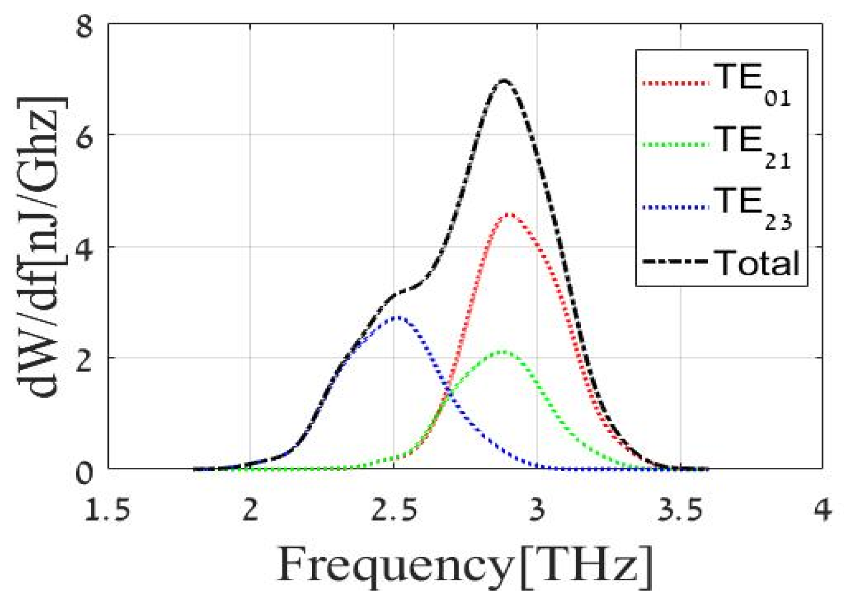
3.1. The EM Field Representation by Eigenmodes

As previously mentioned, the EM pulse consists of many modes, of which the most energetic modes (as shown in Figure 3 above) directly affect the nature and dimensions of the TL. The size and location of the mirrors are directly affected by the propagation of these modes. In this study, the propagation effect of each mode was distinguished separately in a TL of meters (Figure 4).

3.2. The Modes Propagation in Terms of Rays

3.2.1. The TE₀₁ Mode Propagation

The TE₀₁ mode is reminiscent in shape of a rectangular slot (as shown in Figure 5); hence, it is expected that the shape of the interference will be similar to the rectangular slot [40]:

$$\mathrm{I}\left(x,y\right)=I_0{sinc}^2{\displaystyle \frac{D_{x}x\pi }{\lambda z}}{sinc}^2{\displaystyle \frac{D_{y}y\pi }{\lambda z}}$$

(27)

where D_x, D_y is a slot size. According to Equation (27), one can see a “sinc behavior” of the $\pm \left|E\right|=\sqrt{I}$. The greater the length of the slot parameter (D_x, D_y) causes greater decay in this particular axis. Fourier transform of rectangular field apertures and highlighted that this serves as a first-order approximation consistent with the field structure in the TE₀₁ mode.

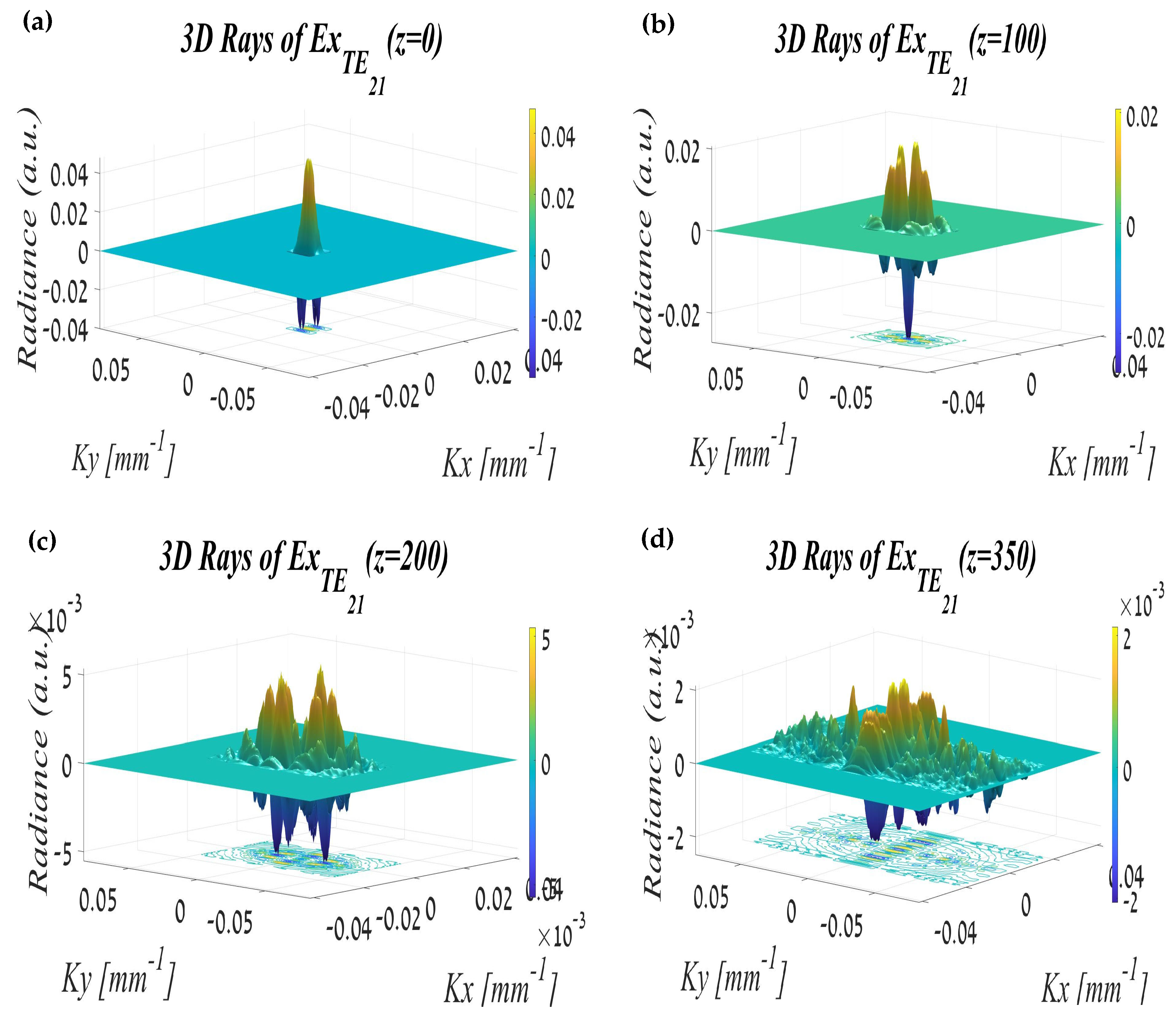
3.2.2. The TE₂₁ Mode Propagation

Propagation in free space of the TE₂₁ mode in Figure 6 resembles in its form the interference of three sources, and the propagation is almost identical in both directions.

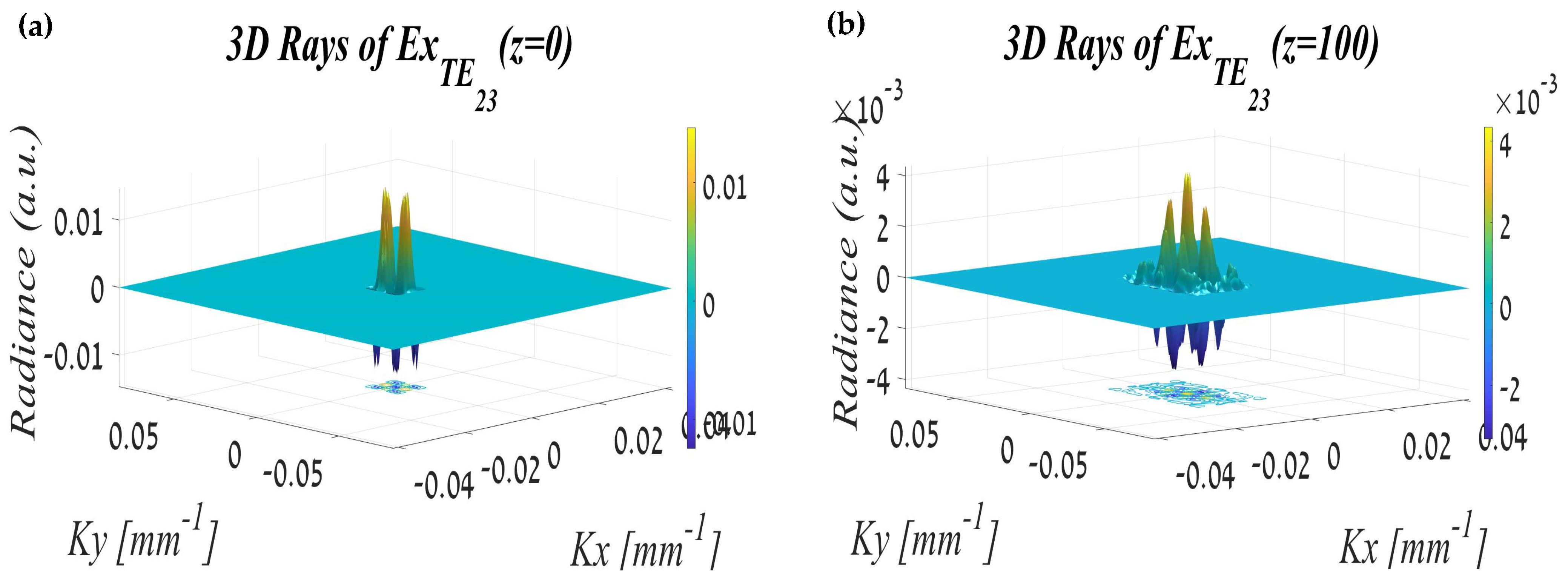
3.2.3. The TE₂₃ Mode Propagation

In Figure 7 it can be clearly seen that TE₂₃ is the most influential mode in terms of the dispersion propagation. This is reflected in a wide angular spread (as can be seen in Figure 7d).

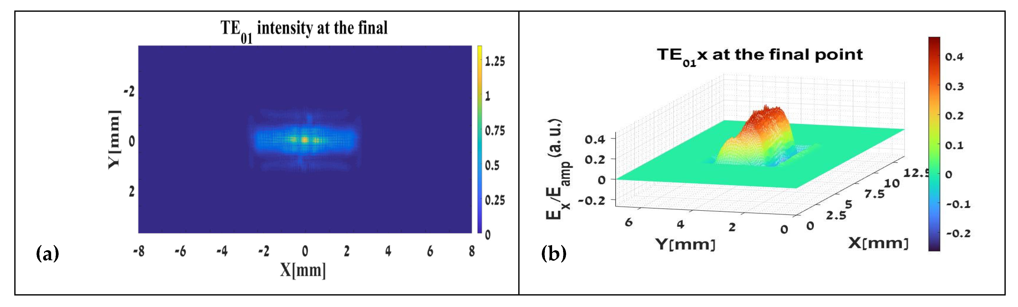
3.3. The Modes’ Reconstruction from Rays at Target Point

Figure 8b,d,f present the results at the end of the TL. In other words, they illustrate the expected field distribution at the user end—on the experimental table of the THz-FEL system. The spatial profiles bear some resemblance to their respective sources, particularly in the TE₀₁ and TE₂₁ modes. Notably, the reconstructed field distributions appear more tightly focused. However, for a direct comparison with the analytical Gaussian beam calculations, we refer to the intensity distributions shown in Figure 8a,c,e.

In all three modes, the beam diameter at the optical path’s exit is approximately one-third of its initial diameter (i.e., reduced from 12 mm to ~4 mm). It should be emphasized that the intensity values have been normalized to the initial peak intensity. Consequently, in the TE₀₁ and TE₂₁ modes, the peak intensity is approximately 1.3 times higher than the initial maximum, reflecting enhanced focusing. In contrast, the TE₂₃ mode reaches only about 70% of its initial peak, a result attributed to the substantial divergence of this mode. Specifically, while 2500 rays were initially launched from each XY coordinate, the most focused pixel at the end of the optical path collected only 1188 rays—demonstrating the broader spatial dispersion of TE₂₃.

4. Discussion

In this work, the TL for a THz Free Electron Laser (FEL) was analyzed through computational modeling using Zemax and Matlab. The analysis focused on three dominant TE modes that carry the majority of the beam’s energy. Using this approach, we studied the electric field distribution and corresponding intensity (power) for each mode.

The simulation results reveal a significant optical divergence: after every 100 mm, the beam’s cross-sectional area is approximately doubled. By 350 mm from the waveguide exit, the rays extend beyond the original aperture. This highlights a key engineering constraint—radiation must be refocused before 350 mm. Consequently, the installation of a focusing mirror at this point becomes imperative. This is the first critical design parameter from which subsequent confocal distances and beam path points can be derived.

The selected method of beam propagation via WDF and discrete rays proved effective. It allowed us to visualize beam direction, intensity, shape, and spatial boundaries clearly. Since the WDF preserves the structure of the original field, it serves as a powerful and reliable tool for optical path planning, particularly in designing quasi-optical systems such as the TL.

Although the detailed design of the TL falls beyond the scope of this work, we can affirm that the conceptual design—based on analytical equations and modeling—has proven valid. The critical focusing point was clearly observed, confirming the accuracy and utility of the RT approach.

The study will proceed by defining the optical and mechanical boundaries of the TL. This involves balancing technical and economic constraints:

• Mirror diameter: Smaller mirrors are more cost-effective and easier to fabricate, especially for THz frequencies. However, the longer propagation distances required for focusing impose larger beam diameters, which can increase both the cost and complexity.
• Pipe dimensions: The vacuum pipes enclosing the TL must endure pressure, adding another layer of engineering constraints.

Each significant mode was analyzed independently to determine scattering limits. This is because reconstructing the full field through the WDF involves cross-terms and interference effects between modes, which are more complex to interpret. A mode-by-mode analysis enables clearer identification of propagation boundaries and design thresholds.

Key findings from this work:

• A TL for THz FEL radiation was conceptually designed and tested based on its dominant TE modes.
• The focal lengths of four parabolic off-axis mirrors were determined. The resulting input/output beam size ratio was approximately 1:4.
• Beam imaging using Matlab and Zemax validated the spatial electric field and power distribution.
• The system design strongly depends on the technical constraints.
• The initial waist radius ω ≈ 3.5 mm is a preliminary estimate. Once the FEL is operational, this parameter must be re-evaluated to finalize the system design.
• The modeled system is largely wavelength-independent under the paraxial approximation, as the ABCD matrix method assumes small angular deviations. However, rays with larger initial angles will show greater wavelength dependence. These rays, however, exhibit lower intensity in the WDF, and thus have a minimal effect on the overall system performance.

5. Conclusions

This study demonstrated the successful simulation of field and intensity distributions for various TE modes propagating through a quasi-optical TL designed for a THz Free Electron Laser (FEL). The approach—combining WDF analysis with ray tracing in Zemax and Matlab—proved effective in evaluating both the optical performance and the physical constraints of the system. The method is generalizable and suitable for a wide range of broadband THz sources, particularly multi-mode, tunable FELs. The use of the Wigner distribution function combined with ray tracing offers a universal phase-space approach to characterize field propagation in any quasi-optical system, independent of specific geometry or mode content. The method is particularly useful for pulsed and coherent THz radiation.

Key achievements include the following:

• Design and Modeling: A TL consisting of four off-axis parabolic mirrors was designed. The focal lengths and relative spacing were optimized to achieve an input/output beam size ratio of approximately 1:4. This configuration facilitates effective mode transmission across a range of wavelengths under paraxial approximation.
• Field Visualization: Simulation of three dominant TE modes (carrying most of the beam’s energy) provided detailed insight into electric field and intensity (power) distributions. The WDF-based representation preserved the spatial structure of the field, enabling robust evaluation of beam behavior throughout the optical system.
• Design Validation: The modeling indicated that the beam diverges significantly after 350 mm, necessitating a focusing mirror within that range. This finding was critical for validating the initial analytical design and establishing design parameters for future iterations.
• Engineering Trade-offs: The optimization is closely linked to physical constraints, such as mirror and pipe diameters, which affect both cost and performance. For instance, increasing mirror diameter improves focusing, but at the expense of fabrication complexity and system footprint.
• Wavelength Independence: While the TL was modeled under the paraxial approximation (using ABCD matrices), the approach remains largely wavelength-independent for small-angle rays. High-angle rays, more sensitive to wavelength, contribute less to the overall field due to their lower intensity in the WDF framework.

This work also highlights the potential for future development:

• Integrated Software Toolchain: A fully automated software framework could be developed to streamline the workflow. Such a tool would take input parameters (mode type and wavelength), interface Matlab and Zemax for beam propagation simulation, and return processed results—significantly improving design efficiency and repeatability.
• Next Steps: After further refinement of the TL design and upon completion of the FEL assembly, it will be essential to repeat the simulations using updated parameters. This includes reassessing the initial waist radius (ω ≈ 3.5 mm), which significantly impacts beam evolution and focusing accuracy.

In summary, the method presented here provides a robust simulation framework for analyzing and designing quasi-optical systems for THz applications. It enables the accurate prediction of beam propagation characteristics and offers a valuable foundation for the continued development of high-performance THz beamlines.

References

1. Dalzell, D.R.; Mcquade, J.; Vincelette, R.; Ibey, B.; Payne, J.; Roach, W.P.; Roth, C.L.; Wilmink, G.J. Damage thresholds for terahertz radiation. In Optical Interactions with Tissues and Cells XXI; SPIE: San Francisco, CA, USA, 2014. [Google Scholar]
2. Siegel, P.H. Terahertz Technology in Biology and Medicine. IEEE Trans. Microw. Theory Tech. 2004, 52, 2438–2447. [Google Scholar] [CrossRef]
3. Sun, Q.; He, Y.; Liu, K.; Fan, S.; Parrott, E.P.J.; Pickwell-MacPherson, E. Recent advances in terahertz technology for biomedical applications. Quant. Imaging Med. Surg. 2017, 7, 345–355. [Google Scholar] [CrossRef] [PubMed]
4. Fitzgerald, A.J.; Wallace, V.P.; Jimenez-Linan, M.; Bobrow, L.; Pye, R.J.; Purushotham, A.D.; Arnone, D.D. Terahertz Pulsed Imaging of Human Breast Tumors. Radiology 2006, 239, 533–540. [Google Scholar] [CrossRef] [PubMed]
5. Yu, C.; Fan, S.; Sun, Y.; Pickwell-Macpherson, E. The potential of terahertz imaging for cancer diagnosis: A review of investigations to date. Quant. Imaging Med. Surg. 2012, 2, 33–45. [Google Scholar]
6. Dieing, T.; Hollricher, O.; Toporski, J. Confocal Raman Microscopy; Springer Series in Optical Sciences: Preface; Springer: Berlin/Heidelberg, Germany, 2010; Volume 158. [Google Scholar]
7. Chamberlain, M.; Jones, B.; Wilke, I.; Williams, G.; Parks, B.; Heinz, T.; Siegel, P. Opportunities in THz Science. Science 2004, 80, 123. [Google Scholar]
8. Tripathi, S.R.; Miyata, E.; Ishai, P.B.; Kawase, K. Morphology of human sweat ducts observed by optical coherence tomography and their frequency of resonance in the terahertz frequency region. Sci. Rep. 2015, 5, 9071. [Google Scholar] [CrossRef]
9. Friedman, A.; Balal, N.; Bratman, V.; Dyunin, E.; Lurie, Y.; Magory, E.; Gover, A. Configuration and status of the israeli THz free electron laser. In Proceedings of the 36th International Free Electron Laser Conference FEL, Basel, Switzerland, 25–29 August 2014; pp. 553–555. [Google Scholar]
10. Gerasimov, M.; Dyunin, E.; Gerasimov, J.; Ciplis, J.; Friedman, A. Application of wigner distribution function for THz propagation analysis. Sensors 2022, 22, 240. [Google Scholar] [CrossRef]
11. Guo, S.; Hu, C.; Zhang, H. Unidirectional ultrabroadband and wide-angle absorption in graphene-embedded photonic crystals with the cascading structure comprising the Octonacci sequence. J. Opt. Soc. Am. B 2020, 37, 2678. [Google Scholar] [CrossRef]
12. Burtsev, V.D.; Vosheva, T.S.; Khudykin, A.A.; Ginzburg, P.; Filonov, D.S. Simple low-cost 3D metal printing via plastic skeleton burning. Sci. Rep. 2022, 12, 7963. [Google Scholar] [CrossRef]
13. Mikhailovskaya, A.; Vovchuk, D.; Grotov, K.; Kolchanov, D.S.; Dobrykh, D.; Ladutenko, K.; Bobrovs, V.; Powell, A.; Belov, P.; Ginzburg, P. Coronavirus-like all-angle all-polarization broadband scatterer. Commun. Eng. 2023, 2, 76. [Google Scholar] [CrossRef]
14. Filonov, D.; Barhom, H.; Shmidt, A.; Sverdlov, Y.; Shacham-Diamand, Y.; Boag, A.; Ginzburg, P. Flexible metalized tubes for electromagnetic waveguiding. J. Quant. Spectrosc. Radiat. Transf. 2019, 232, 152–155. [Google Scholar] [CrossRef]
15. Alonso, M.A. Wigner functions in optics: Describing beams as ray bundles and pulses as particle ensembles. Adv. Opt. Photonics 2011, 3, 272. [Google Scholar] [CrossRef]
16. Gerasimov, M.; Yahya, A.H.; Nave, V.P.; Dyunin, E.; Gerasimov, J.; Friedman, A. Analysis and 3D Imaging of Multidimensional Complex THz Fields and 3D Diagnostics Using 3D Visualization via Light Field. Computation 2023, 11, 160. [Google Scholar] [CrossRef]
17. Lurie, Y.; Friedman, A.; Pinhasi, Y. Single pass, THz spectral range free-electron laser driven by a photocathode hybrid rf linear accelerator. Phys. Rev. Spec. Top. Accel. Beams 2015, 18, 1–9. [Google Scholar] [CrossRef]
18. Pinhasi, Y.; Lurie, Y.; Yahalom, A. Space-frequency model of ultrawide-band interactions in free-electron lasers. Phys. Rev. Spec. Top. Accel. Beams 2005, 8, 1–8. [Google Scholar] [CrossRef]
19. Sumithra, P.; Thiripurasundari, D. A review on Computational Electromagnetics Methods. Adv. Electromagn. 2017, 6. [Google Scholar] [CrossRef]
20. Samad, M.A.; Choi, S.W.; Kim, C.S.; Choi, K. Wave Propagation Modeling Techniques in Tunnel Environments: A Survey. IEEE Access 2023, 11, 2199–2225. [Google Scholar] [CrossRef]
21. Gerasimov, J.; Balal, N.; Liokumovitch, E.; Richter, Y.; Gerasimov, M.; Bamani, E.; Pinhasi, G.A.; Pinhasi, Y. Scaled modeling and measurement for studying radio wave propagation in tunnels. Electronics 2021, 10, 53. [Google Scholar] [CrossRef]
22. Wigner, E. On the quantum correction for thermodynamic equilibrium. Phys. Rev. 1932, 40, 749–759. [Google Scholar] [CrossRef]
23. Bastiaans, M.J. The Wigner distribution function applied to optical signals and systems. Opt. Commun. 1978, 25, 26–30. [Google Scholar] [CrossRef]
24. Shabtay, G.; Mendlovic, D.; Zalevsky, Z. Proposal for optical implementation of the Wigner distribution function. Appl. Opt. 1998, 37, 2–4. [Google Scholar] [CrossRef] [PubMed]
25. Tanner, G.; Ramapriya, D.M.; Gradoni, G.; Creagh, S.C.; Moers, E.; Lopéz Arteaga, I. A Wigner function approach to near-field acoustic holography—Theory and experiments. In Proceedings of the Inter-Noise 2019 Madrid—48th International Congress and Exposition on Noise Control Engineering, Madrid, Spain, 16–19 June 2019. [Google Scholar]
26. Dragoman, D. Applications of the Wigner Distribution Function. EURASIP J. Adv. Signal Process. 2005, 2005, 1520–1534. [Google Scholar] [CrossRef]
27. Orovi, I.; Stankovi, S.; Dragani, A. Time-frequency based analysis of wireless signals. In Proceedings of the 2012 Mediterranean Conference on Embedded Computing, Bar, Montenegro, 19–21 June 2012. [Google Scholar]
28. Yang, Z.; Qiu, W.; Sun, H.; Nallanathan, A. Robust radar emitter recognition based on the three-dimensional distribution feature and transfer learning. Sensors 2016, 16, 289. [Google Scholar] [CrossRef]
29. Sun, K.; Jin, T.; Yang, D. An improved time-frequency analysis method in interference detection for GNSS receivers. Sensors 2015, 15, 9404–9426. [Google Scholar] [CrossRef]
30. Alonso, M. Exact description of free electromagnetic wave fields in terms of rays. Opt. Express 2003, 11, 3128. [Google Scholar] [CrossRef]
31. Jepsen, P.U.; Cooke, D.G.; Koch, M. Terahertz spectroscopy and imaging—Modern techniques and applications. Laser Photonics Rev. 2011, 166, 124–166. [Google Scholar] [CrossRef]
32. Lakshminarayan, V.; Calvo, M.L.; Alieva, T. Mathematical Optics: Classical, Quantum, and Computational Methods; CRC Press: Boca Raton, FL, USA, 2012; pp. 13–51. [Google Scholar]
33. Torre, A. Linear Ray and Wave Optics in Phase Space: Bridging Ray and Wave Optics via the Wigner Phase-Space Picture; Elsevier: Amsterdam, The Netherlands, 2005. [Google Scholar]
34. Gershun, A. The Light Field. J. Math. Phys. 1939, 18, 51–151. [Google Scholar] [CrossRef]
35. Levoy, M. Light fields and computational imaging. Computer 2006, 39, 46–55. [Google Scholar] [CrossRef]
36. Dragoman, D.; Peiponen, K.-E. (Eds.) Terahertz Spectroscopy and Imaging; Springer Series in Optical Sciences 171; Springer: Berlin/Heidelberg, Germany, 2013. [Google Scholar]
37. Kapilevich, B.; Lurie, Y.; Perutski, B.; Litvak, B.; Etinger, A.; Friedman, A. Radiation Fields of THz Free Electron Laser: 3D EM Simulation and Experimental Study. In Proceedings of the 2014 IEEE 28th Convention of Electrical & Electronics Engineers in Israel, Eilat, Israel, 3–5 December 2014; pp. 28–31. [Google Scholar]
38. Gerasimov, M.; Perutski, B.; Dyunin, E.; Gerasimov, J.; Friedman, A. Visualization of an Ultra-Short THz Beams with a Radiation Propagation Analysis of the Novel Israeli Free Electron Laser. Computation 2022, 10, 193. [Google Scholar] [CrossRef]
39. Horowits, O.; Gerasimov, M.; Lurie, Y.; Friedman, A. Study of the transmission line for Israeli THz free-electron radiation source. Phys. Plasmas 2022, 29, 113301. [Google Scholar] [CrossRef]
40. Saleh, B.E.A.; Teich, M.C. Fundamentals of Photonics, 3rd ed.; John Wiley & Sons, Inc.: Hoboken, NJ, USA, 2019. [Google Scholar]
Figure 1. THz FEL setup at the Schlesinger Center.
Electronics 14 02506 g001
Figure 2. THz transmission line.
Electronics 14 02506 g002
Figure 3. Output amplitude radiation spectrum of Israeli free-electron THz source.
Electronics 14 02506 g003
Figure 4. The EM field at the waveguide output: (a) TE01 mode; (b) TE21, and (c) TE23 modes.
Electronics 14 02506 g004
Figure 5. The TE01 mode propagation in terms of the rays: (a) at the out of the waveguide, (b) after passing 100 mm, (c) after passing 200 mm, and (d) after passing 350 mm.
Electronics 14 02506 g005
Figure 6. The TE21 mode propagation in terms of the rays: (a) at the out of the waveguide, (b) after passing 100 mm, (c) after passing 200 mm, and (d) after passing 350 mm.
Electronics 14 02506 g006
Figure 7. The TE23 mode propagation in terms of the rays: (a) at the out of the waveguide, (b) after passing 100 mm, (c) after passing 200 mm, and (d) after passing 350 mm.
Electronics 14 02506 g007aElectronics 14 02506 g007b
Figure 8. The modes’ intensity and pattern (shape), respectively: (a,b) TE01, (c,d) TE21, and (e,f) TE23 at the TL’s end from the ray reconstruction (inverse WDF).
Electronics 14 02506 g008aElectronics 14 02506 g008b
Disclaimer/Publisher’s Note: The statements, opinions and data contained in all publications are solely those of the individual author(s) and contributor(s) and not of MDPI and/or the editor(s). MDPI and/or the editor(s) disclaim responsibility for any injury to people or property resulting from any ideas, methods, instructions or products referred to in the content.