Low-Cost Robust Detection Method of Interturn Short-Circuit Fault for Distribution Transformer Based on ΔU-I Locus Characteristic

Abstract

Winding interturn short-circuit (ISCF) fault is a common problem which occurs in distribution transformers due to multiple internal and external factors. Unfortunately, the variations in electric parameters under a slight fault are tiny and hardly used as effective characteristics for the detection and protection system. To address this issue, a low-cost robust detection method of ISCF based on the port voltage–current (ΔU-I) locus characteristic is presented in this paper. The mathematical model of the three-phase distribution transformer with ISCF is first established. Then, the ΔU-I locus function and relevant characteristic parameters are analyzed, respectively, which can reflect the healthy and faulty conditions. The axis length ratio between the major axis length and the minor axis length in the ΔU-I ellipse curve is defined as the fault indicator for the sensitivity and robustness of fault diagnosis. Moreover, this method can reduce the number of sensors and has strong robustness against load fluctuations. In the end, the theoretical analysis and simulation results verify the effectiveness of the ΔU-I locus characteristic.

1. Introduction

Distribution transformer is a kind of critical and numerous equipment in electricity grids, which plays a key role in the field of power transmission and voltage conversion [1,2,3]. Once the power supply is interrupted due to a transformer fault, it may cause an outage, safety accidents, and a series of serious consequences [4]. During the operation of the transformer, overvoltage, poor heat dissipation of the winding, incomplete impregnation of insulating paper, or water mixed in the oil will lead to the deterioration of the insulation performance between turns of the winding. Then, the interturn short-circuit fault might be formed, which will contribute to complete insulation breakdown and interphase short-circuit fault in serious cases [5,6].

ISCF is a common fault type of oil-immersed power transformer, and the main cause of interturn fault is the aging or deterioration of insulation [7]. Historical statistics indicate that the probability of ISCF accounts for a large proportion of transformer winding faults [8]. For the initially slight ISCF, the interturn insulation has not broken down, and the interturn insulation resistance still has a high resistance value, which makes the change in winding current not obvious. Although it may not cause an accident immediately, it will bring about the degradation of the health state of the transformer winding, and then reduce the reliability of the operation [9,10]. Consequently, it is necessary to adopt preventative measures to monitor the actual state of power transformers and identify hidden faults.

Existing techniques to identify winding faults of distribution transformers are mainly divided into offline detection methods and online monitoring methods [11]. The traditional offline detection methods for winding fault diagnosis include short-circuit impedance (SCI) [12], low-voltage impulse [13], and sweep frequency response analysis (SFRA) [14,15]. Among these detection techniques, the prominent problem is that they are all offline in nature and call for the disconnection of the transformer for testing. Nonetheless, the randomness and rapid progression of ISCF in transformer windings usually render conventional offline inspections ineffective for failure prevention, due to limited temporal resolution in fault detection [16].

For the necessity of continuously monitoring the winding status, a growing number of scholars have been devoted to exploring online detection methods of winding faults. Present schemes of online monitoring transformer winding ISCF can be roughly divided into online FRA [15,17], inference by vibration (IV) [18,19], embedded sensors (ES) [20,21], and port voltage–current characteristics (ΔU-I) [22,23]. The online FRA method can detect most winding faults in real time, but the measured signals are often influenced by various factors such as load level, stray capacitance, and bushing characteristics [24]. Ref. [25] shows that the diagnostic accuracy of the IV method depends on the precision of the sensor and the installation position because vibration sensors need to be installed on the surface of the transformer. Furthermore, the ES method is an invasive scheme, which requires customizing special transformers and increases overall cost [26]. As an online and noninvasive technique, the ΔU-I locus characteristics method is proposed, and it utilizes the existing metering devices attached to power transformers, which do not demand additional equipment or sensors [27]. However, there are relatively few studies on this part. In [23,27], the slant angle or eccentricity of the ΔU-I ellipse curve is considered as the single fault indicator, which is easily disturbed by load fluctuations and is not sensitive enough to detect slight ISCF. The changes in the fault indicators before and after the ISCF are slight, making it difficult to set an appropriate threshold. Furthermore, it is necessary to collect data on high voltage and large current in the above method.

In addition to the methods mentioned above, the use of artificial intelligence (AI) in power transformer monitoring is another emerging scheme. Ref. [28] proposes a boundary wavelet coefficient energy of the differential and restraining currents to detect the fault. In [29], it uses the actual value obtained from the terminal measurements to compare with the healthy transformer model to detect the presence of ISCF [30]. Innovatively utilizes advanced metaheuristic algorithms to determine the optimal angles that yield the best distribution of samples, offering a more reliable tool for fault diagnosis in oil-immersed transformers. However, the methods based on AI rely on complex algorithms and a large amount of historical operational data. It is challenging and inconvenient for online real-time monitoring.

In this article, a low-cost, robust detection method is proposed to diagnose ISCF for the distribution transformer, which depends on the axis length ratio of the ΔU-I locus characteristic. The calculation of the axis length ratio requires the primary winding voltage, which is estimated instead of measured. Therefore, the system cost can be reduced, which is the first contribution of this article. Meanwhile, the proposed method is robust to load fluctuations, which is the second contribution of this article. The rest of this article is organized as follows. The mathematical model and ΔU-I locus curve are given in Section 2. Section 3 outlines the ΔU-I locus curve characteristics and construction of the fault indicator, then assesses its sensitivity and reliability. Section 4 presents the simulation verification with different fault severities and load levels to verify the effectiveness of the proposed method. Finally, the conclusion is drawn in Section 5.

2. Theoretical Analysis

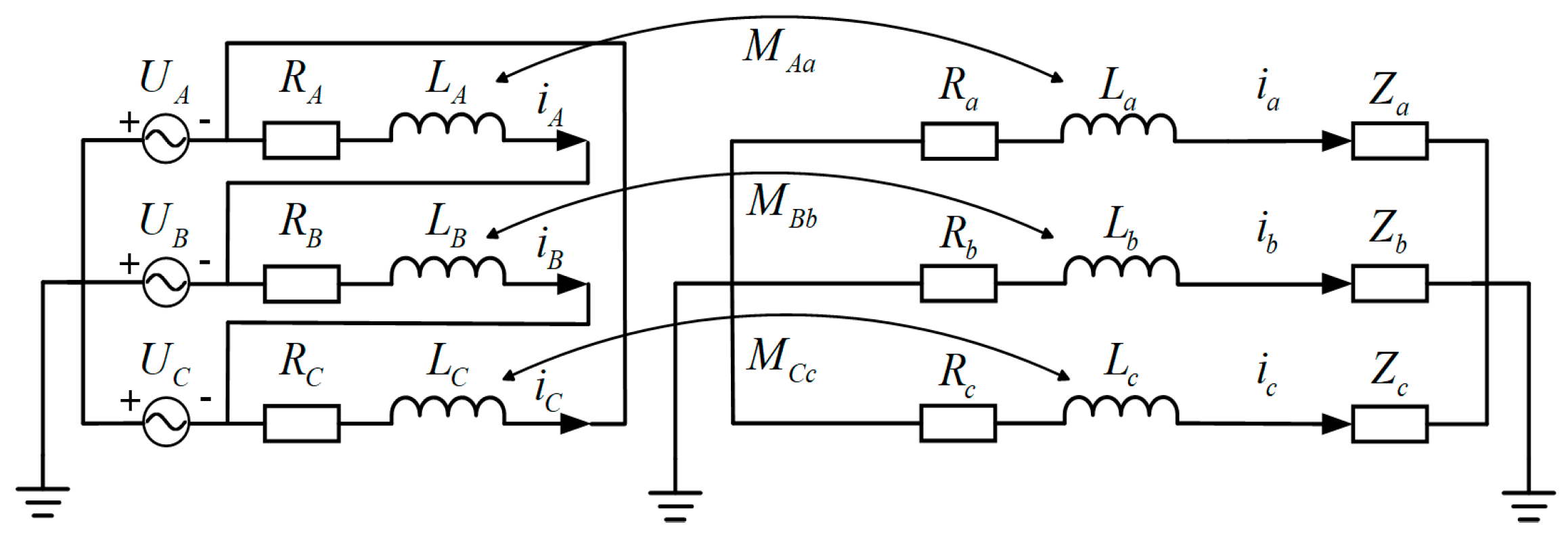
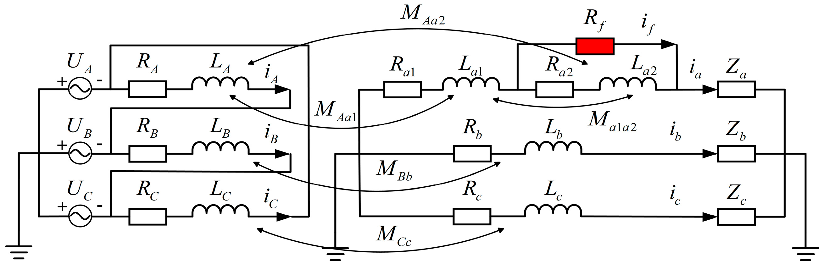
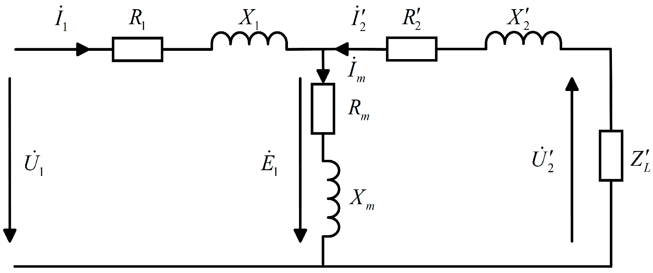
2.1. The ISCF Model of Three-Phase Transformer

In this section, the 10/0.4 kV distribution transformer commonly used in the power distribution network is selected as the main research object. The equivalent circuit model of the transformer under healthy conditions is shown in Figure 1. The primary winding of the transformer is connected in a triangular configuration, while the secondary winding is connected in a star configuration. R represents the resistance of the winding, L represents the leakage inductance, and Z represents the load impedance. As seen in Figure 1, the winding connection group symbol of the three-phase transformer model is Dyn11, in which the capitalized subscript “_X” represents the phase-X of the primary winding and the lowercase subscript “_x” corresponds to the phase-x of the secondary winding.

According to Figure 1, the expression of the transformer state space can be deduced as

$${\displaystyle \frac{di}{dt}}=A_{s}i(t)+B_{s}U(t)$$

(1)

where i = [i_A, i_B, i_C, i_a, i_b, i_c]^T is composed of the winding current of each phase, U = [U_A, U_B, U_C, 0, 0, 0]^T is the voltage vector. A_s and B_s are state matrices and input matrices of the transformer under different operating conditions and can be represented as

$$\left\{\begin{array}{l}{A}_s={\left[\begin{array}{cc}{L}_{11}\hfill & \hfill L_{12}\hfill \\ L_{21}\hfill & \hfill L_{22}+L_{load}\hfill \end{array}\right]}^{-1}\left[\begin{array}{cc}-R_{11}\hfill & \hfill 0\hfill \\ \hspace{0.17em}\hspace{0.17em}0\hfill & \hfill -R_{22}-R_{load}\hfill \end{array}\right]\hfill \\ B_s={\left[\begin{array}{cc}{L}_{11}\hfill & \hfill L_{12}\hfill \\ L_{21}\hfill & \hfill L_{22}+L_{load}\hfill \end{array}\right]}^{-1}\hfill \end{array}\right.$$

(2)

where R_load and L_load∈R^{3 × 3} consist of load impedance, R₁₁ and R₂₂∈R^{3 × 3} are diagonal matrices composed of the resistance of each phase on the primary winding and secondary winding, respectively, and L₁₁, L₂₂, L₁₂, and L₂₁∈R^{3 × 3} are the block array of inductance matrix including self-inductance and mutual inductance between the primary winding and secondary winding.

Figure 2 displays the equivalent circuit model in which the ISCF is assumed to be in the secondary winding of phase-a. In this model, the leakage impedance of each phase and the mutual inductance between the primary winding and the secondary windings are taken into account. The ISCF of winding can be modeled by adding an additional circuit, including contact resistance R_f to the faulty turns in phase-a, which simulates the degree of insulation deterioration. Otherwise, i_f is used to describe the circulating current of short-circuit turns. The original secondary winding is divided into a healthy part and a faulty part, which are, respectively, denoted by subscripts ‘’₁” and “₂”. The resistance matrix is extended to a fourth-order diagonal matrix as follows:

$$R_{22}=\mathrm{diag}(R_{a1},R_{a2},R_b,R_c)$$

(3)

where R_a1 and R_a2 are the resistance of the healthy part and the faulty part. At the same time, the inductance matrix is extended to 7 × 7 order, and the voltage matrix is extended to U = [U_A, 0, U_B, U_C, 0, 0, 0]^T.

Because the ISCF is introduced to the secondary phase-a winding, the resistance and leakage inductance of this phase winding are bound to change, thus affecting the amplitude and phase of the port voltage and current. In most cases, the mutual inductance between different phases of a power transformer is tiny and can be ignored. Hence, the ISCF in one phase generally does not significantly affect the port voltages and currents of the other two phases.

2.2. ΔU-I Locus Function

In this section, the ΔU-I locus function is introduced in detail. It is acknowledged that a normally operating power transformer usually has the property of three-phase symmetry [31]. Without loss of generality, it is acceptable to research only one phase of the distribution transformer. The simplified T-type equivalent circuit of a single-phase transformer is presented in Figure 3. For the normal operation with load, the parameters of the secondary windings can be converted to the primary side as follows:

$$\left\{\begin{array}{c}{\dot{U}}_2^{\prime }=k{\dot{U}}_2\\ {\dot{I}}_2^{\prime }={\dot{I}}_2/k\\ Z_L^{\prime }=k^2{Z}_L\end{array}\right.$$

(4)

where k is the ratio of the voltage of the primary winding to that of the secondary winding.

Assuming that load impedance Z_L = R_L + jX_L is a resistive-inductive load, it can be concluded that the initial phase of the input current lags behind that of the input voltage, while the initial phase of the output current lags behind the output voltage. Therefore, the vector diagram corresponding to the single-phase equivalent circuit diagram can be obtained and presented in Figure 4.

According to Figure 4, the initial phase of the primary winding voltage can be set to θ_u1. The initial phase difference between the voltage of the secondary winding and that of the primary winding is α, and that between the current of the secondary winding and the voltage of the primary winding is β. Next, the mathematical expressions of port voltage and current after normalization are as follows:

$$\left\{\begin{array}{l}{u}_1^{*}(t)=u_1(t)/U_{1N}=U_1^{*}\sin (\omega t+{\theta }_{u1})\hfill \\ u_2^{*}(t)=u_2(t)/U_{2N}=U_2^{*}\sin (\omega t+{\theta }_{u1}-\alpha )\hfill \\ i_2^{*}(t)=i_2(t)/I_{2N}=I_2^{*}\sin (\omega t+{\theta }_{u1}-\beta )\hfill \end{array}\right.$$

(5)

where the superscript “$*$” refers to per-unit values to omit the transformer turns ratio, while the subscript “_N” represents the rated value, the subscript “₁” indicates the primary winding, and “₂” represents the secondary winding. Otherwise, these port data are the phase voltage or phase current of the transformer winding.

The ΔU-I method proposes the construction of a locus diagram between the instantaneous values of $\left(u_1^{*}-u_2^{*}\right)$ and $i_2^{*}$. At the same time, the voltage difference between the input voltage and the output voltage can be simplified and combined by mathematical methods, so these parameters can be rewritten as

$$\left\{\begin{array}{l}{u}_1^{\ast }(t)-u_2^{\ast }(t)=\Delta u^{\ast }\left(t\right)=\Delta U_p^{\ast }\sin \left(\omega t+{\theta }_1\right)\hfill \\ {i_2}^{\ast }(t)=I_p^{\ast }\sin \left(\omega t+{\theta }_2\right)\hfill \end{array}\right.$$

(6)

where symbols θ₁ and θ₂ are adopted to represent the initial phase of the voltage difference and the output current, respectively, for consistency, subscript “_p” represents the peak value.

The variable ωt can be omitted in the following way:

$$\begin{array}{c}\omega t=\arcsin \left({\displaystyle \frac{\Delta u^{*}}{\Delta U_p^{*}}}\right)-{\theta }_1=\arcsin \left({\displaystyle \frac{i_2^{*}}{I_p^{*}}}\right)-{\theta }_2\\ \Rightarrow \arcsin \left({\displaystyle \frac{\Delta u^{*}}{\Delta U_p^{*}}}\right)=\arcsin \left({\displaystyle \frac{i_2^{*}}{I_p^{*}}}\right)+{\theta }_1-{\theta }_2\end{array}$$

(7)

Finally, the ΔU-I locus function in this paper can be derived from (7) and derivation is shown in the Appendix A.

$${\displaystyle \frac{\Delta u^{*2}}{\Delta U_p^{*2}}}-{\displaystyle \frac{2\cos ({\theta }_1-{\theta }_2)\Delta u^{*}{i}_2^{*}}{\Delta U_p^{*}{I}_p^{*}}}+{\displaystyle \frac{i_2^{*2}}{I_p^{*2}}}-{\sin }^2\left({\theta }_1-{\theta }_2\right)=0$$

(8)

where $\Delta u^{*}$ and $i_2^{*}$ are variables in the Formula (8), and the other parameters are all constant coefficients under certain operating conditions. In order to make the (8) look more concise and convenient, the letters A, B, C, and D are used to replace the four coefficients in the formula as follows:

$$\left\{\begin{array}{l}A={\displaystyle \frac{1}{\Delta U_p^{*2}}}\hfill \\ B=-{\displaystyle \frac{2\cos ({\theta }_1-{\theta }_2)}{\Delta U_p^{*}{I}_p^{*}}}\hfill \\ C={\displaystyle \frac{1}{I_p^{*2}}}\hfill \\ D=-{\sin }^2\left({\theta }_1-{\theta }_2\right)\hfill \end{array}\right.$$

(9)

Based on the above coefficients, the Formula (8) can be concisely expressed as

$$A\Delta u^{*2}+B\Delta u^{*}{i}_2^{*}+C{i}_2^{*}+D=0$$

(10)

Further, the following (11) holds true for all cases, thus the relationship between $\Delta u^{*}$ and $i_2^{*}$ represents an ellipse locus.

$$B^2-4AC={\displaystyle \frac{4}{\Delta U_p^{*2}{I}_p^{*2}}}\left[{\cos }^2({\theta }_1-{\theta }_2)-1\right]<0$$

(11)

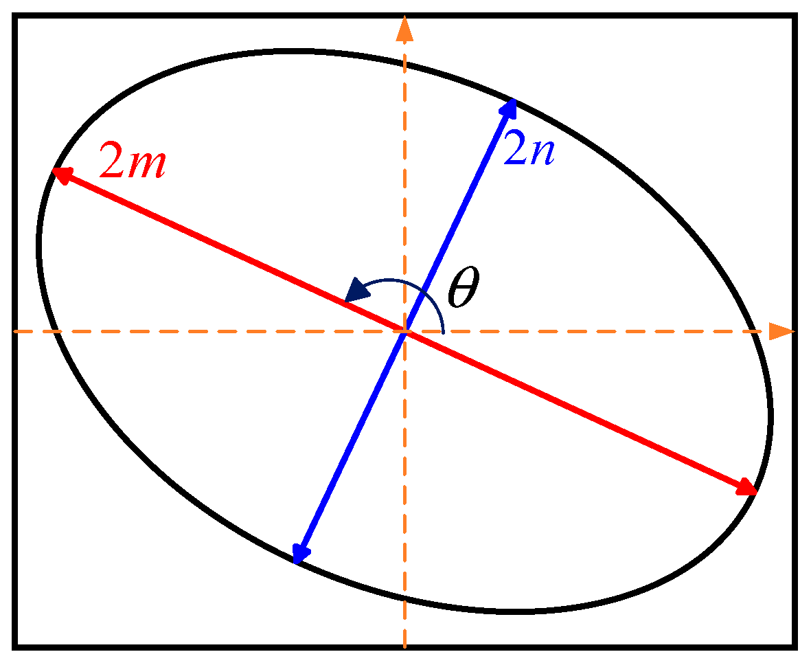
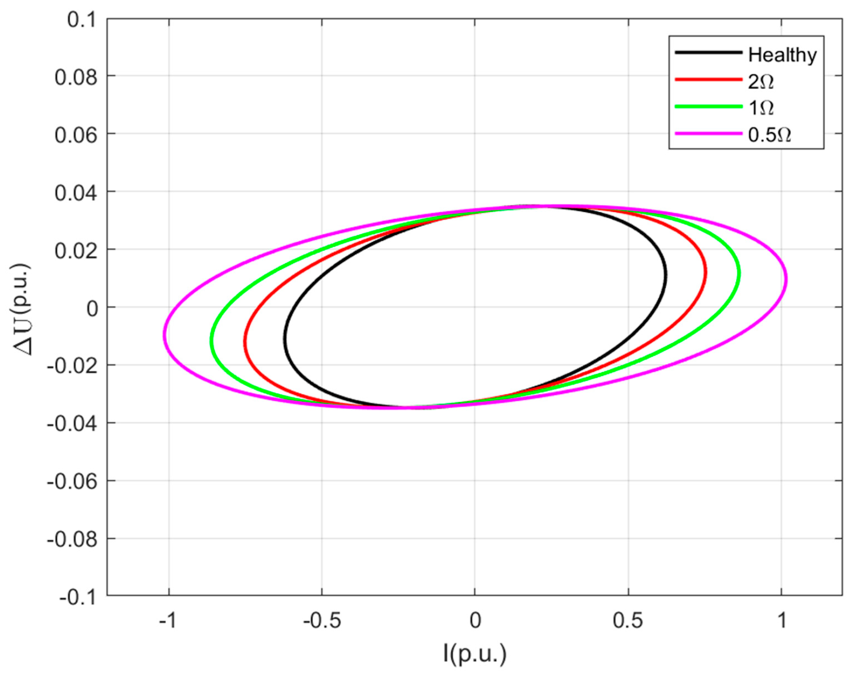
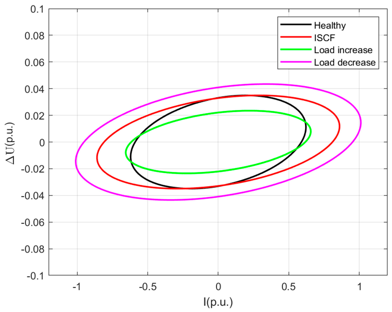
2.3. Ellipse Curve Characteristics

The ellipse curve characteristics for fault diagnosis will be presented in this section. Figure 5 presents the ellipse slant angle (θ), major axis length (m), and minor axis length (n), all of which are characteristic parameters of the ΔU-I ellipse curve. Furthermore, the eccentricity is also one of the prominent parameters of an ellipse. They can be deduced from (10) as follows:

$$\theta =\arctan ({\displaystyle \frac{B}{A-C}})/2$$

(12)

$$m=\sqrt{-2D/\left[A+C-\sqrt{B^2+{(A-C)}^2}\right]}$$

(13)

$$n=\sqrt{-2D/\left[A+C+\sqrt{B^2+{(A-C)}^2}\right]}$$

(14)

$$e=\sqrt{1-n^2/m^2}$$

(15)

If the ISCF occurs in the one-phase winding of a transformer, the coefficients in (9) will change, thereby causing these characteristic parameters (12)–(15) to differ from the healthy operation condition. Theoretically, it is possible to diagnose whether ISCF has occurred or not by setting an appropriate threshold.

3. Proposed Detection Method

3.1. Fault Indicator

The T-type equivalent circuit diagram presented in Figure 3 is commonly used to analyze the one-phase transformer operation. In fact, the magnetizing current of a power transformer under healthy and normal operation is tiny and would not affect the overall analysis process. Hence, it is reasonable to remove the magnetizing branch from Figure 3. The equivalent circuit diagram after further simplification is shown in Figure 6.

According to Figure 6, the parameters in the Formula (9) can be obtained as

$$\left\{\begin{array}{l}{\dot{U}}_1-{\dot{U}}_2^{\prime }={\dot{I}}_1{Z}_k={\dot{I}}_2^{\prime }{Z}_k\hfill \\ \Delta U_p^{*}=I_p^{*}\times \left|Z_k\right|\hfill \\ {\theta }_1-{\theta }_2=\arg (Z_k)\hfill \end{array}\right.$$

(16)

From (9) and (16), the characteristic parameters of the ΔU-I ellipse curve can be represented as

$$\left\{\begin{array}{l}\theta ={\displaystyle \frac{1}{2}}\arctan \left[2\left|Z_k\right|\cos (\arg (Z_k))/({\left|Z_k\right|}^2-1)\right]\hfill \\ m={\displaystyle \frac{{\left|Z_k\right|}^2{I}_p^{*2}}{1+2\left|Z_k\right|\cos (\arg (Z_k))\tan \theta +{\left|Z_k\right|}^2\tan \theta }}\hfill \\ n={\displaystyle \frac{{\left|Z_k\right|}^2{I}_p^{*2}}{{\left|Z_k\right|}^2+2\left|Z_k\right|\cos (\arg (Z_k))\tan \theta +\tan \theta }}\hfill \end{array}\right.$$

(17)

Equation (17) indicates that the ellipse slant angle (θ) is independent of the load fluctuations, but the major axis length (m) and minor axis length (n) will be affected. Because the amplitude of the secondary winding current is determined by the load level. In previous research, the ellipse slant angle or eccentricity is used for ISCF diagnosis. In this article, the ratio of m to n is defined as the fault indicator, which has better diagnostic sensitivity than θ under a slight ISCF condition. The subsequent simulation results will also illustrate this conclusion. In the meantime, the fault indicator will not be interrupted by load fluctuations due to the fact that the division operation eliminates the current.

$$FI={\displaystyle \frac{m}{n}}={\displaystyle \frac{{\left|Z_k\right|}^2+2\left|Z_k\right|\cos (\arg (Z_k))\tan \theta +\tan \theta }{1+2\left|Z_k\right|\cos (\arg (Z_k))\tan \theta +{\left|Z_k\right|}^2\tan \theta }}$$

(18)

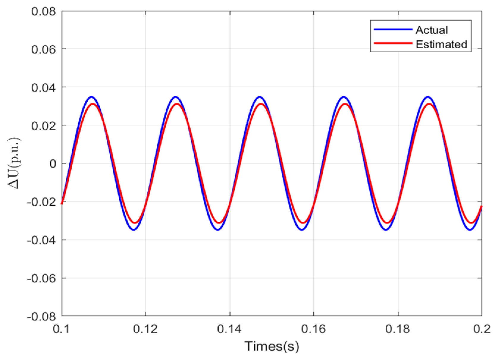
3.2. Low-Cost Phase Voltage Estimator

According to Formula (5), there are three types of data that need to be collected, including the primary winding voltage, primary winding current, and secondary winding voltage. In general, the amplitudes of the primary winding current and the secondary winding voltage are smaller than the primary winding voltage. Therefore, it is easier to collect and convert them into signals that the controller can handle. For distribution transformers, the primary winding voltages are all in the range of several tens of kilovolts, which are pretty difficult to measure in practice. This section will introduce how to reduce three types of data into two types, that is, only the primary winding current and the secondary winding voltage.

In the previous section, it was mentioned that during healthy and normal operation, the magnetizing current ${\dot{I}}_m$ and magnetizing branch of the transformer can be disregarded. When ${\dot{I}}_m$ is equal to 0, ${\dot{I}}_1$ can be equivalent to ${\dot{I}}_2^{\prime }$, and Δ is also equal to β in Figure 4. Hence, the phase difference between ${\dot{U}}_2^{\prime }$ and ${\dot{I}}_1$(${\dot{I}}_2^{\prime }$) is just caused by the load impedance, while the phase difference between ${\dot{U}}_1$ and ${\dot{I}}_1$ is jointly determined by the equivalent impedance of the load and the windings. If Z_k and Z’_L are known, the phase difference between the primary winding voltage and the current can be derived by

$$\delta =\arctan {\displaystyle \frac{R_k+R_L^{\prime }}{X_k+X_L^{\prime }}}=\arctan {\displaystyle \frac{R_k+k^2{R}_L}{X_k+k^2{X}_L}}$$

(19)

where $R_k=R_1+R_2^{\prime }=R_1+k^2{R}_2$ is the equivalent resistance of the transformer winding, $X_k=X_1+X_2^{\prime }=X_1+k^2{X}_2$ is the equivalent reactance. They can be calculated as

$$Z_k={\displaystyle \frac{U_k}{I_k}}={\displaystyle \frac{U_k\%\times U_{1N}}{I_{1N}}}$$

(20)

$$R_k={\displaystyle \frac{P_k/3}{I_k^2}}={\displaystyle \frac{P_k}{3I_{1N}^2}}$$

(21)

$$X_k=\sqrt{Z_k^2-R_k^2}$$

(22)

where U_k% is short-circuit impedance voltage percentage and P_k is load loss. They were measured through short-circuit experiments and the results will be given in the name plate of the transformer. U_1N and I_1N are rated values and can be calculated from the rated capacity, thus they are also known parameters.

Based on Figure 6, the state equation of a single-phase transformer in load operation is

$${\dot{U}}_2={\dot{I}}_2{Z}_L$$

(23)

In the meantime, it can be approximately viewed that the phase angles of ${\dot{I}}_1$ and ${\dot{I}}_2$ are the same when the magnetizing current ${\dot{I}}_m$ is ignored. After obtaining the data of the primary winding current, it is multiplied by the transformation ratio k of the transformer to obtain the current of the secondary winding is feasible. The equivalent impedance of the load can be expressed as

$$Z_L={\displaystyle \frac{U_2}{I_2}}={\displaystyle \frac{U_2}{k{I}_1}}$$

(24)

$$R_L=Z_L\times \cos ({\theta }_{u2}-{\theta }_{i2})\approx Z_L\times \cos ({\theta }_{u2}-{\theta }_{i1})$$

(25)

$$X_L=Z_L\times \sin ({\theta }_{u2}-{\theta }_{i2})\approx Z_L\times \sin ({\theta }_{u2}-{\theta }_{i1})$$

(26)

It should be noted that when calculating the equivalent impedance of the windings and the load mentioned, the amplitude or the effective value should be uniformly adopted. So far, all the parameters required for calculating the Δ in (19) have been obtained.

In addition, it is known that the primary windings of the transformer are directly connected to the power grid [32], while the secondary windings are connected to the users. In large power grid systems, voltage fluctuations are relatively small, so it can be considered that the voltage of the primary windings remains near the rated value. As a result, the amplitude of $u_1^{*}(t)$ in (5) is equal to 1, and the phase is the sum of Δ and the phase of the primary winding current.

Through the above analysis, we only need to acquire the data of the primary winding current and the secondary winding voltage to calculate the fault indicator because the primary winding voltage can be derived from the primary winding current.

4. Simulation Validation and Performance Analysis

To verify the effectiveness of the proposed detection method, its performances are compared with that of the conventional detection method [23,27]. For the conventional detection method, it is usually necessary to use a potential transformer and a voltage sensor together to collect the primary winding voltage, and the primary wingding current and secondary wingding voltage can be obtained from common sensors. Then, these three types of data are used to calculate the ellipse slant angle online. However, in this article, only the primary winding current and the secondary winding voltage are required to calculate the axis length ratio. The schematic diagram of the proposed monitoring method framework is shown in Figure 7.

The following simulation results are performed based on the simulation platform MATLAB/Simulink 2021a, and the main parameters of the transformer are listed in

Table 1. Name plate parameters of the transformer.

Parameter	Value
Model number	S13-M-400
Number of phases	3
Connection group symbol	Dyn11
Rated capacity	400 kVA
Rated frequency	50 Hz
Rated voltage	10/0.4 kV
No-load power loss	200 W
Load power loss	4520 W
No-load current	0.5%
Short-circuit impedance voltage	4.0%

. In order to describe the severity of ISCF, the shorted turn ratio and fault resistance are introduced in this paper. The subsequent results are all based on the assumption that ISCF is introduced to the middle position of the primary winding in phase-b of the transformer. Otherwise, the module called Multi-Winding Transformer in Simulink is adopted, the time step is set to 0.0001 s, and the solver used is ode45. During the signal acquisition process, a low-pass filter is used in the simulation model to remove high-frequency noise signals, and the interference has become very minimal.

In Figure 8, the simulation results of the voltage difference ΔU waveform are presented. The blue waveform represents the one drawn using the actual primary winding voltage, while the red waveform is obtained by utilizing the phase voltage estimator. It is proven that the performance of the phase voltage estimator is great, which can estimate the actual primary winding voltage.

Figure 9 presents the comparison of the ΔU-I locus curve between the conventional detection method and the proposed method. The two trajectory curves are almost completely overlapping. Under healthy and normal operation, the proposed method for reducing sensors has the same effect as the conventional method.

Figure 10 presents the ΔU-I locus curve under different shorted turn ratios, in which the fault resistance is always equal to 2Ω. The corresponding shorted turn ratio for a healthy transformer is zero. With the increase in shorted turn ratio, the ΔU-I ellipse curve rotates clockwise, and the slant angle θ decreases simultaneously. Meanwhile, the shape of the ellipse has changed significantly, and the length of its major axis has increased. The comparison results of slant angle θ and fault indicator FI versus different shorted turn ratios have been presented in

Table 2. Comparison of fault diagnosis indexes versus different shorted turn ratios.

Method	Healthy	4%	8%	12%
Conventional method θ	1.0227°	0.9287°	0.6305°	0.3824°
Proposed method FI	18.7716	22.9750	33.7263	48.4405

. It is observed that variation in FI is greater than that of θ, which has a better diagnostic performance by setting a suitable threshold value.

In Figure 11, the fault resistance is reduced from 2 Ω to 0.5 Ω while the shorted turn ratio remains 4%. Similarly,

Table 3. Comparison of fault diagnosis indexes versus different fault resistances.

Method	Healthy	2 Ω	1 Ω	0.5 Ω
Conventional method θ	1.0226°	0.9294°	0.7823°	0.5493°
Proposed method FI	18.7716	22.9639	26.1650	30.2084

lists the comparison results of θ and FI with diverse fault resistances. The data in Table 3 also shows that the fault indicator in this paper is more sensitive than the slant angle under the same fault severity.

In addition, based on the data in Table 2 and Table 3, it can be seen that under the same level of fault severity, the absolute value and relative percentage of the change in the proposed fault indicator FI are both greater than those of the conventional method θ. Therefore, the proposed method is more sensitive.

To prove the fault indicator is reliable under load fluctuations, Figure 12 presents the simulation results when the load of the transformer in a healthy condition increases and decreases. The ΔU-I ellipse curve is completely distinct from ISCF, which appears to have been proportionally enlarged or condensed. The relevant fault diagnosis indexes are given in

Table 4. Comparison of fault diagnosis indexes under load fluctuation.

Method	Healthy	Load Increase	Load Decrease
Conventional method θ	1.0229°	1.0225°	1.0226°
Proposed method FI	18.7716	18.7718	18.7716

. However, the FI is slightly varied when the load fluctuates, indicating that the proposed detection method is robust to most operating conditions.

Figure 13 is intended to demonstrate that the load changes after ISCF have little effect on fault diagnosis results. Therefore, the simulation was carried out to simulate the situations where the load increases and decreases after the occurrence of ISCF. The θ and FI under different operating conditions have been provided in

Table 5. Comparison of fault diagnosis indexes after ISCF with load fluctuation.

Method	Healthy	Faulty	Load Increase	Load Decrease
Conventional method θ	1.0229°	0.7845°	0.6960°	0.8263°
Proposed method FI	18.7716	26.1320	26.7113	25.6996

. Although the load keeps changing, FI still not be influenced by the result of fault diagnosis.

5. Conclusions

This paper proposed a low-cost, robust method for ISCF of the distribution transformer. In the proposed method, the changes in the ΔU-I locus are analyzed before and after ISCF occurs in the primary winding. The robustness of various characteristic Mparameters of the ellipse locus is compared and discussed in detail. Then, the axis length ratio is defined as the fault indicator, taking into account the sensitivity and robustness. Moreover, the proposed method can reduce the number of sensors and has strong robustness against load fluctuations. Finally, the effectiveness of the proposed detection method is verified by simulation results. It is worth noting that the changes in the transformer’s own parameters and non-sinusoidal loads require further investigation in the future.

References

1. Amoiralis, E.I.; Tsili, M.A.; Kladas, A.G. Power Transformer Economic Evaluation in Decentralized Electricity Markets. IEEE Trans. Ind. Electron. 2012, 59, 2329–2341. [Google Scholar] [CrossRef]
2. Meira, M.; Bossio, G.R.; Ruschetti, C.R.; Verucchi, C.J. Inter-Turn Short-Circuit Detection Through Differential Admittance Monitoring in Transformers. IEEE Trans. Instrum. Meas. 2024, 73, 3519508. [Google Scholar]
3. Liu, D.; Wang, Y.; Liu, C.; Yuan, X.; Yang, C.; Gui, W. Data Mode Related Interpretable Transformer Network for Predictive Modeling and Key Sample Analysis in Industrial Processes. IEEE Trans. Ind. Inform. 2023, 19, 9325–9336. [Google Scholar] [CrossRef]
4. Kumar, A.; Bhalja, B.R.; Kumbhar, G.B. Approach for Identification of Inter-Turn Fault Location in Transformer Windings Using Sweep Frequency Response Analysis. IEEE Trans. Power. Del. 2022, 66, 1539–1548. [Google Scholar] [CrossRef]
5. Moradzadeh, A.; Pourhossein, K.; Mohammadi-Ivatloo, B.; Mohammadi, F. Locating Inter-Turn Faults in Transformer Windings Using Isometric Feature Mapping of Frequency Response Traces. IEEE Trans. Ind. Inform. 2021, 17, 6962–6970. [Google Scholar] [CrossRef]
6. Farzin, N.; Vakilian, M.; Hajipour, E. Transformer Turn-to-Turn Fault Protection Based on Fault-Related Incremental Currents. IEEE Trans. Power. Del. 2019, 34, 700–709. [Google Scholar] [CrossRef]
7. Ahmadi, S.-A.; Sanaye-Pasand, M.; Abedini, M.; Samimi, M.H. Online Sensitive Turn-to-Turn Fault Detection in Power Transformers. IEEE Trans. Ind. Electron. 2022, 69, 13555–13564. [Google Scholar] [CrossRef]
8. Bagheri, S.; Moravej, Z.; Gharehpetian, G.B. Classification and Discrimination Among Winding Mechanical Defects, Internal and External Electrical Faults, and Inrush Current of Transformer. IEEE Trans. Ind. Inform. 2018, 14, 484–493. [Google Scholar] [CrossRef]
9. Zhao, Z.; Yao, C.; Li, C.; Islam, S. Detection of Power Transformer Winding Deformation Using Improved FRA Based on Binary Morphology and Extreme Point Variation. IEEE Trans. Ind. Electron. 2018, 65, 3509–3519. [Google Scholar] [CrossRef]
10. Zheng, J.; Huang, H.; Pan, J. Detection of Winding Faults Based on a Characterization of the Nonlinear Dynamics of Transformers. IEEE Trans. Instrum. Meas. 2019, 68, 206–214. [Google Scholar] [CrossRef]
11. Luo, B.; Wang, H.; Liu, H.; Li, B.; Peng, F. Early Fault Detection of Machine Tools Based on Deep Learning and Dynamic Identification. IEEE Trans. Ind. Electron. 2016, 23, 509–518. [Google Scholar] [CrossRef]
12. Masoum, A.S.; Hashemnia, N.; Abu-Siada, A.; Masoum, M.A.S.; Islam, S.M. Online Transformer Internal Fault Detection Based on Instantaneous Voltage and Current Measurements Considering Impact of Harmonics. IEEE Trans. Power Del. 2017, 32, 587–598. [Google Scholar] [CrossRef]
13. Lavrinovich, V.A.; Mytnikov, A.V. Development of pulsed method for diagnostics of transformer windings based on short probe impulse. IEEE Trans. Dielect. Elect. Insul. 2015, 22, 2041–2045. [Google Scholar] [CrossRef]
14. Pham, D.A.K.; Gockenbach, E. Analysis of physical transformer circuits for frequency response interpretation and mechanical failure diagnosis. IEEE Trans. Dielect. Elect. Insul. 2019, 68, 1491–1499. [Google Scholar] [CrossRef]
15. Akhmetov, Y.; Nurmanova, V.; Bagheri, M.; Zollanvari, A.; Gharehpetian, G.B. A New Diagnostic Technique for Reliable Decision-Making on Transformer FRA Data in Interturn Short-Circuit Condition. IEEE Trans. Ind. Electron. 2021, 17, 3020–3031. [Google Scholar] [CrossRef]
16. Ouyang, X.; Zhou, Q.; Shang, H.; Zheng, Y.; Pan, S.; Luo, J. Toward a Comprehensive Evaluation on the Online Methods for Monitoring Transformer Turn-to-Turn Faults. IEEE Trans. Ind. Electron. 2024, 71, 1997–2007. [Google Scholar] [CrossRef]
17. Kumar, A.; Bhalja, B.R.; Kumbhar, G.B. Novel Technique for Location Identification and Estimation of Extent of Turn-to-Turn Fault in Transformer Winding. IEEE Trans. Ind. Electron. 2023, 70, 7382–7392. [Google Scholar] [CrossRef]
18. Shi, Y.; Ji, S.; Zhang, F.; Dang, Y.; Zhu, L. Application of operating deflection shapes to the vibration-based mechanical condition monitoring of power transformer windings. IEEE Trans. Power Del. 2021, 36, 2164–2173. [Google Scholar] [CrossRef]
19. Wu, S.; Ji, S.; Zhang, Y.; Wang, S.; Liu, H. A Novel Vibration Frequency Response Analysis Method for Mechanical Condition Detection of Converter Transformer Windings. IEEE Trans. Ind. Electron. 2024, 71, 8176–8180. [Google Scholar] [CrossRef]
20. Haghjoo, F.; Mostafaei, M.; Mohammadi, H. A new leakage flux-based technique for turn-to-turn fault protection and faulty region identification in transformers. IEEE Trans. Power Del. 2018, 33, 671–679. [Google Scholar] [CrossRef]
21. Venikar, P.A.; Ballal, M.S.; Umre, B.S.; Suryawanshi, H.M. Search coil based online diagnostics of transformer internal faults. IEEE Trans. Power Del. 2017, 32, 2520–2529. [Google Scholar] [CrossRef]
22. Yao, C.; Zhao, Z.; Mi, Y.; Li, C.; Liao, Y.; Qian, G. Improved online monitoring method for transformer winding deformations based on the Lissajous graphical analysis of voltage and current. IEEE Trans. Power Del. 2015, 30, 1965–1973. [Google Scholar] [CrossRef]
23. Zhao, X.; Yao, C.; Zhou, Z.; Li, C.X.; Wang, X.; Zhu, T.; Abu-Siada, A. Experimental Evaluation of Transformer Internal Fault Detection Based on V–I Characteristics. IEEE Trans. Ind. Electron. 2020, 67, 4108–4119. [Google Scholar] [CrossRef]
24. Nurmanova, V.; Bagheri, M.; Zollanvari, A.; Aliakhmet, K.; Akhmetov, Y.; Gharehpetian, G.B. A New Transformer FRA Measurement Technique to Reach Smart Interpretation for Inter-Disk Faults. IEEE Trans. Power Del. 2019, 34, 1508–1519. [Google Scholar] [CrossRef]
25. Wu, S.; Zhang, F.; Dang, Y.; Zhan, C.; Wang, S.; Ji, S. A Mechanical-Electromagnetic Coupling Model of Transformer Windings and its Application in the Vibration-Based Condition Monitoring. IEEE Trans. Power Del. 2023, 38, 2387–2397. [Google Scholar] [CrossRef]
26. Xian, R.; Wang, L.; Zhang, B.; Li, J.; Xian, R.; Li, J. Identification Method of Interturn Short Circuit Fault for Distribution Transformer Based on Power Loss Variation. IEEE Trans. Ind. Inform. 2024, 20, 2444–2454. [Google Scholar] [CrossRef]
27. Abu-Siada, A.; Islam, S. A Novel Online Technique to Detect Power Transformer Winding Faults. IEEE Trans. Power Del. 2012, 27, 849–857. [Google Scholar] [CrossRef]
28. Medeiros, R.P.; Costa, F.B.; Silva, K.M. Power transformer differential protection using the boundary discrete wavelet transform. IEEE Trans. Power Del. 2016, 31, 2083–2095. [Google Scholar] [CrossRef]
29. Tripathy, M.; Maheshwari, R.P.; Verma, H.K. Power transformer differential protection based on optimal probabilistic neural network. IEEE Trans. Power Del. 2015, 30, 1007–1015. [Google Scholar] [CrossRef]
30. Hechifa, A.; Labiod, C.; Lakehal, A.; Nanfak, A.; Mansour, D.-E.A. A Novel Graphical Method for Interpretating Dissolved Gases and Fault Diagnosis in Power Transformer Based on Dynamique Axes in Circular Form. IEEE Trans. Power Del. 2024, 39, 3186–3198. [Google Scholar] [CrossRef]
31. Kumar, A.; Bhalja, B.R.; Kumbhar, G.B. A New Improved Methodology to Identify an Interturn Fault Location in Transformer Winding Based on Fault Location Factor. IEEE Trans. Ind. Electron. 2024, 71, 15024–15033. [Google Scholar] [CrossRef]
32. Bhalja, H.; Bhalja, B.R.; Agarwal, P.; Malik, O.P. Time–Frequency Decomposition Based Protection Scheme for Power Transformer— Simulation and Experimental Validation. IEEE Trans. Ind. Electron. 2024, 71, 5296–5306. [Google Scholar] [CrossRef]
Figure 1. Dyn11 connection transformer under healthy conditions.
Electronics 14 02458 g001
Figure 2. Dyn11 connection transformer with ISCF in phase-a.
Electronics 14 02458 g002
Figure 3. T-type equivalent circuit diagram of a single-phase transformer.
Electronics 14 02458 g003
Figure 4. Vector diagram of a single-phase transformer.
Electronics 14 02458 g004
Figure 5. Elliptical curve and characteristic parameters.
Electronics 14 02458 g005
Figure 6. Simplified equivalent circuit diagram.
Electronics 14 02458 g006
Figure 7. Schematic diagram of the proposed method.
Electronics 14 02458 g007
Figure 8. ΔU waveform comparison of actual condition and estimated condition.
Electronics 14 02458 g008
Figure 9. Comparison between the conventional detection method and the proposed method.
Electronics 14 02458 g009
Figure 10. ΔU-I locus curve versus different shorted turn ratios.
Electronics 14 02458 g010
Figure 11. ΔU-I locus curve versus different fault resistances.
Electronics 14 02458 g011
Figure 12. ΔU-I locus curve versus under load fluctuation condition.
Electronics 14 02458 g012
Figure 13. ΔU-I locus curve after ISCF with load fluctuation.
Electronics 14 02458 g013