Deep Neural Network Confidence Calibration from Stochastic Weight Averaging

Abstract

Overconfidence in deep neural networks (DNN) reduces the model’s generalization performance and increases its risk. The deep ensemble method improves model robustness and generalization of the model by combining prediction results from multiple DNNs. However, training multiple DNNs for model averaging is a time-consuming and resource-intensive process. Moreover, combining multiple base learners (also called inducers) is hard to master, and any wrong choice may result in lower prediction accuracy than from a single inducer. We propose an approximation method for deep ensembles that can obtain ensembles of multiple DNNs without any additional costs. Specifically, multiple local optimal parameters generated during the training phase are sampled and saved by using an intelligent strategy. We use cycle learning rates starting at 75% of the training process and save the weights associated with the minimum learning rate in every iteration. Saved sets of the multiple model parameters are used as weights for a new model to perform forward propagation during the testing phase. Experiments on benchmarks of two different modalities, static images and dynamic videos, show that our method not only reduces the calibration error of the model but also improves the accuracy of the model.

1. Introduction

During training, a deep neural network (DNN) learns the output probability, which indicates the DNN’s confidence in the results. Some recent work has found that the confidence of a DNN is not consistent with its accuracy [1,2,3]. These works point out that DNNs suffer from overconfidence. An overconfident DNN gives high confidence in wrong predictions. The problem of overconfidence poses a huge challenge to the deployment of DNNs in real-world applications. For example, in health care, criminal justice, and autonomous driving applications, we expect models to have a certain degree of confidence in their predictions in order to make more informed decisions. Confidence calibration not only enhances the model’s ability to generalize and minimizes potential risks but also greatly aids in its interpretability [4,5].

Confidence calibration is the process of adjusting the predicted probabilities of a model to better reflect the true likelihood of its predictions being correct [2,6]. More formally, a completely calibrated classification model is one in which the probability of the predicted outcome $\widehat{Y}$ being equal to the actual outcome Y is defined as $\mathbb{P}(\widehat{Y}=Y\mid \widehat{P}=p)=p$, where p falls within the range of $[0,1]$, and $\widehat{P}$ is the model’s associated confidence. It is expected that $\widehat{P}$ will be calibrated, indicating that it accurately reflects an actual probability. An accurately-calibrated classifier is a probabilistic classifier that can be directly interpreted in terms of confidence score through its predicted probability output. To illustrate, a precisely calibrated (binary) classifier that yields 100 samples with a confidence score of $0.6$ for every prediction indicates that 60 samples will be accurately classified. Confidence calibration refers to a model’s capacity to accurately assign probabilities to its predictions [7]. In recent years, multiple techniques have been introduced to generate predictive confidence scores through calibration [2,8,9], including post-processing, Bayesian neural networks, and deep ensemble methods. Temperature scaling is a post-processing calibration method proposed by Guo et al. [2]. The main principle revolves around the utilization of a singular scalar parameter, $T>0$, denoting the temperature, to modify the logit score prior to the implementation of the softmax function. The method cannot effectively handle out-of-distribution data because T is computed on the validation set. The idea behind the Bayesian neural network approach is to infer the probability distribution of the DNN parameters. This distribution is used to sample the parameters for single forward propagation, resulting in random predictions that are influenced by diverse model weights. However, precise Bayesian inference is computationally difficult for neural networks and incurs extremely expensive computational and memory costs [3].

Deep ensemble learning [10] combines the predictions of several base estimators to reduce the variance of predictions and reduce generalization errors. The concept of ensembling is based on the idea that a group of models can work together to enhance the strengths and minimize the weaknesses of individual base learners. Deep ensembles were originally proposed and discussed to improve the prediction performance of DNNs. In [11], the authors, through the experimental analysis of several regression and classification tasks, showed that averaging the predictions of ensemble models can also be used to derive useful uncertainty estimates. Moreover, in [12], deep ensembles were shown to be state-of-the-art for the domain shift (or out-of-distribution) setting. Compared to single-model methods [2], the computational costs and memory consumption of the deep ensemble approach are significantly higher. Moreover, the additional computations increase linearly with the number of base learners. Some interesting methods, such as distillation, sub-ensembles, and batch ensembles, have been proposed to solve these problems. However, these approaches necessitate substantial changes to the training process and remain costly in regards to both time and computational resources. To overcome these challenges, work in [13] presented an approximate method to implement an ensemble of models without increasing the training cost. During the training phase, multiple snapshots of the model are periodically saved, and the predictions from the multiple snapshots are averaged during the testing phase. Instead of training M models from scratch, the snapshot ensembles in [13] were created by changing the learning rate to allow the optimizer to reach the local minimum M times during the optimization process. In [14], the study demonstrated that simple curves connect the optima of complex loss functions, with consistent training and test accuracy. Based on this geometric finding, they proposed a new approximate ensembling procedure called fast geometric ensembling (FGE). The FGE algorithm uncovers various networks by taking small steps in the weight space while remaining in a low test error region. FGE allows training of highly effective ensembles in the same amount of time it takes to train a single model. However, these single-model multiple-weight methods were initially proposed to improve the accuracy of the DNN but with little attention paid to confidence in the output. It remains unclear whether these methods are effective in reducing confidence errors.

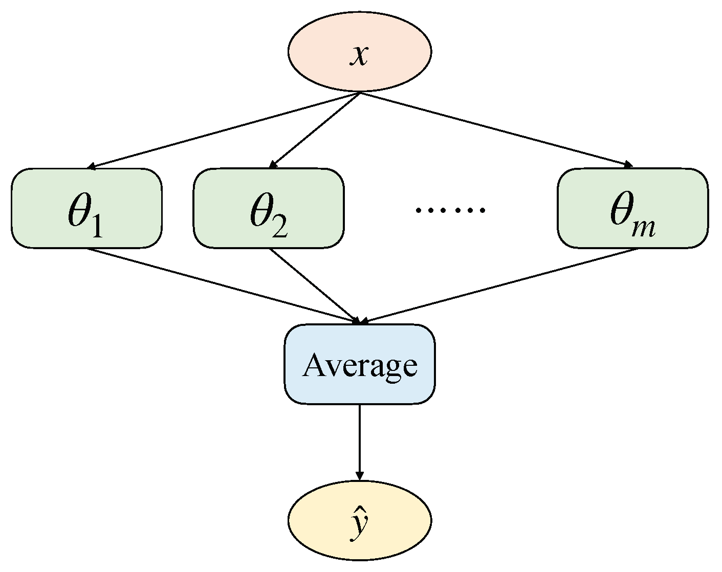
To fill this gap, we propose a confidence calibration method based on stochastic weight averaging. We achieve this by training a single DNN to converge to multiple local minima on the loss surface and to sample and save the model parameters by using a smart strategy. At a high level, the concept of averaging the stochastic gradient descent (SGD) iterations has been around for several decades in the field of convex optimization [9,15]. In convex optimization, researchers have primarily focused on optimizing convergence rates by implementing averaged SGD. In deep learning, the use of averaged SGD results in a smoother trajectory for SGD iterations but yields minimal differences in performance. By contrast, we are more concerned in this work with the effect of the method on the calibration error. Multiple locally optimal weights generated in the training phase are specially sampled, and then forward propagation is computed as new parameters for the base learner during the testing phase. We force the optimizer to explore a variety of models rather than converge on just one solution by using a modified learning rate strategy. We use a smart strategy to select relatively more meaningful weights from a large number of candidate weights. To summarize, instead of designing multiple sets of DNNs, the method simply trains a single model to obtain well-calibrated confidence output. We tested our method on two benchmarks with varying modalities, including static images and dynamic videos. Our experimental findings indicate that our method effectively minimizes calibration error and enhances the model’s precision. The code is publicly available at github.com/zjcao/swaCal (accessed on 22 January 2024).

The main contributions of our work are summarized as follows.

(1)

We propose an alternate ensemble learning approach to improve the quality of neural network uncertainty measures to overcome overconfidence without incurring additional computational costs.

(2)

We evaluate our approach using two benchmarks with different modalities: static images and dynamic videos. The results of our experiments demonstrate that our approach successfully reduces calibration error and enhances the model’s accuracy.

The remainder of this paper is structured as follows. Section 2 discusses related studies on deep ensemble learning and confidence calibration. Section 3 describes our proposed approach in detail. The experiments and results are presented in Section 4. Section 5 is the conclusion and suggests further studies.

2. Related Work

2.1. Confidence Calibration of a Deep Neural Network

Confidence calibration is a sub-task of open-set recognition that aims to improve the accuracy of confidence scores for DNN output. DNN output is the probability during an inference process that indicates the model’s confidence in the result. A precisely calibrated confidence can represent the probability that the predicted label is correct. Although DNNs have obtained good prediction accuracy in a variety of visual tasks, recent studies have found that DNNs suffer from overconfidence [2,7,8]. For a classification task, data scientists usually use softmax output (predicted probability) as the true probability of correctness in the predicted category. This might have been reasonable for traditional network models in the past, but it is not applicable to the DNNs of today. In [16], the authors found that passing a point estimate through the softmax function produced a high probability. After that, Guo et al. [2] found the same problem and demonstrated through a series of ablation experiments that model depth and width, batch normalization, and weight decay have strong effects on the confidence calibration of DNNs. The process of calibrating a classifier involves creating a calibrator that translates the classifier’s output into a calibrated probability ranging from 0 to 1. The calibrator attempts to predict the conditional probability of the event, $p(y_i=1/f_i$) based on the classifier’s output, $f_i$, for a specific sample.

The confidence calibration methods can be classified into three types depending on the approach: (a) regularization methods during the training phase, (b) post-processing methods after the training phase, and (c) DNN-based uncertainty estimation methods. Regularization-based confidence calibration methods are performed by changing the objective function or by augmenting the training dataset during the DNN training process. Label smoothing, data augmentation, and objective function modification are three commonly used methods for confidence calibration based on regularization [17,18,19]. On the other hand, various methods have been developed in the last decade to recalibrate model confidence through post-processing steps. Temperature scaling, proposed in [2], is a simple and effective technique for recalibrating the prediction probability of modern neural networks. The core algorithm used for temperature scaling rescales the logit value, $f_i\left(x\right)$, by using a single scale parameter, T (temperature), before passing it to the softmax function: $softmax(f_i/T)$. T is extracted by minimizing the negative log-likelihood on the validation datasets after the model training is complete. Although temperature scaling is an effective way to quantify the total predictive uncertainty of calibrated probabilities, it cannot capture the uncertainty caused by out-of-distribution data [12]. By decreasing model uncertainty, the confidence prediction of a DNN can be better calibrated. The rationale for this is that the remaining uncertainty in the predicted data more accurately reflects the true uncertainty in the prediction. Bayesian and ensemble methods are two methods that are used to estimate model uncertainty. The key idea of the Bayesian method is to infer the probability distribution over the model parameters. The prior distribution of the neural network parameters is specified, and then the posterior distribution of the parameters is calculated using the training data. Finally, the uncertainty of the model is predicted according to Bayesian theory. The main challenge for Bayesian deep learning is to specify meaningful conjugate priors for the parameters. Moreover, exact Bayesian inference is often computationally difficult for neural networks with a large number of parameters. Therefore, approximate Bayesian inference techniques, such as variational inference, Laplace approximation, and Markov chain Monte Carlo (MC), are usually used to calculate posterior probabilities [1,6]. Although the Bayesian neural network can estimate the uncertainty of the prediction, the inference phase procedure requires substantial modification due to the inclusion of Bayes’ law. In addition, specifying meaningful priors for Bayesian neural networks is a big challenge [3,4].

2.2. Deep Ensemble Learning

The deep ensemble learning approach merges the benefits of deep learning and ensemble learning, resulting in a final model with improved generalization abilities [20]. The main idea behind deep ensemble learning is that by combining several models, the deficiency of a single base learner may be compensated for by other base learners so the overall predictions of the ensemble are better than a single base learner. The ensemble method for deep learning is roughly divided into two steps: (1) training different models (the training phase) and (2) merging prediction results (the inference phase). In the training phase, multiple models can be obtained using different model architectures, training data, and training strategies. In the inference phase, the same input can be provided to the model for the prediction. Finally, the prediction of each model is combined according to a certain strategy to obtain the final prediction. The deep ensemble method can usually be one of two types: the averaging method and the boosting method [5,6]. The core idea of the averaging method is to build several estimators independently and then average their predictions, as is performed in the bagging method and random forest. Boosting methods such as AdaBoost and gradient tree boosting create the base estimators sequentially to reduce the bias of the combined models. Boosting and random forest are classical machine learning ensemble techniques and complementary methods [21].

In deep learning, dropout is designed as a regularization technique for neural networks to avoid overfitting, which can also be interpreted as an ensemble of multiple models. In [16], the authors showed that MC dropout can be used to quantify the uncertainty of the model. However, in [11], the authors found that in various datasets and tasks of regression and classification, deep ensemble methods were superior to MC dropout in quantifying uncertainty. Furthermore, the deep ensemble method has been shown to be robust in quantifying uncertainty for data beyond distribution [12,22]. However, the computational costs and memory consumption of the ensemble method are significantly higher than in other methods. Therefore, how to effectively reduce the computational workload and memory consumption has become a new research topic in the area of ensemble methods. Pruning methods [23] reduce the complexity of the ensemble by pruning members and reducing redundancy among members. Other approaches, such as batch ensembles and sub-ensembles, attempt to reduce computational cost and memory usage by sharing portions among individual members. We propose an approximate ensemble learning approach that is simple to implement, requires very little hyperparameter tuning, and achieves comparable performance.

3. Confidence Calibration

3.1. Approximate Deep Ensemble Learning

Confidence calibration is the degree to which the uncertainty of the prediction matches the true underlying uncertainty in the data. The softmax probability score is commonly employed by scientists as a confidence metric for the predictions in image classification tasks. Studies have shown that DNN prediction scores can be either overly confident or lacking in confidence. Deep ensemble learning methods reduce prediction variance and improve robustness and generalization by combining prediction results from multiple DNNs constructed using a specific learning strategy. The main principle behind the ensemble approach is to construct several independent estimators and then average their predictions to yield the final prediction. Due to its reduced variance, the combined estimator achieves better results than any single base estimator. Formally, given sample x, the ensemble prediction, $p\left(y\right|x)$, is estimated by averaging the predictions of all the models, which can be expressed as $p\left(y\right|x)=\frac{1}{M}{\sum }_{i=1}^M{p}_i\left(y|x\right)$, where $p_i\left(y\right|x)$ is the predicted output of the i-th base estimator, and m is the number of models in deep ensemble learning. It has been shown that a DNN ensemble can improve the robustness and accuracy of the system compared to using individual networks. However, the computational burden of training multiple DNNs for the ensemble is considerable. Mastering the combinations of ensemble models can be challenging, and an incorrect selection could lead to reduced prediction accuracy compared to using a single model.

On the other hand, in [11], the authors showed that the utilization of an ensemble method for averaging DNN predictions can provide reliable estimates of uncertainty. In addition, the authors in [12] pointed out that a deep ensemble not only performs well in quantifying the uncertainty of a model but also has good robustness against out-of-distribution data. However, little attention has been paid to whether the confidence in the output predictions of ensemble models is representative of the true probability. The ensemble method requires more training time and computations compared to other confidence calibration methods, such as Bayesian neural networks and the post-calibration method.

We propose using the approximate ensemble method to calibrate the confidence of DNNs. We utilize a cyclical learning rate to collect models that are spatially close to each other but that produce diverse predictions. Instead of individually training multiple base estimators, our method performs a single supervised training session to obtain well-calibrated confidence scores. Assume that the training data, D, has N pairs of independent and identically distributed samples, denoted $D={\{x_n,y_n\}}_{n=1}^N$, where $x\in {\mathbb{R}}^d$ represents the d-dimensional features, while y is the label for a classification task and is one of K classes (i.e., $y\in \{1,\dots ,K\}$). Given the input data, x, our task is to use the DNN to model the probabilistic predictive distribution of the labels, $p_{\theta }\left(y\right|x)$, where $\theta$ is the weight parameters of the DNN. During the training phase, we utilize the training set D to conduct standard supervised learning on the model via the proper scoring rules (which is further explained in later sections). The parameters of DNNs are often several orders of magnitude greater than the training data points. That is, they include a large possible function space that may be very close to the data generation function. Thus, there are multiple low-loss valleys (local optimums) during the whole learning period, all corresponding to good but different functions (here, we call them candidate functions). These candidate functions represent varying assumptions used to determine the underlying fundamental function. The more candidate functions in the ensemble, the more likely it is to represent the truth, thus, constructing a more robust model. Figure 1 shows the schematic of the loss landscape based on SGD optimization. We can see that several local optima appear throughout the training process. Note that the valley where the loss finally arrives is not considered the global optimum either.

The weights of the model are updated several times in each iteration cycle. The sampling and saving of these weights are intuitively important to our method. In general, four metrics are counted in each iteration cycle: training accuracy, training loss, validation accuracy, and validation loss. Instead of saving the model using the validation accuracy, we are using a cyclic learning rate for the last 25% training times and saving the network weights corresponding to the lowest value of the learning rate in each cycle. That is, when we save the model we only care whether the current cycle learning rate is at its lowest. Afterwards, we perform stochastic weighted averaging on the multiple sets of weights obtained.

3.2. Stochastic Weighted Averaging

During the training stage, the multiple local optimal weights generated during the training process are sampled and simulated as new parameters of the base learner for inference. Since the loss trajectories and weight values are different, this leads the ensemble model to make diverse predictions. After the training stage, we save m model weights, ${\theta }_1,{\theta }_2,\dots ,{\theta }_m$ each of which are used in the final ensemble. Figure 2 illustrates the data flow of fusion of our approach. In the inference phase, the given input is fed to multiple base learners to predict output. The parameters of the multiple base learners are sampled from the training process by a smart sampling strategy. The method allows for the training of highly effective ensembles in the same amount of time it takes to train a single DNN.

In this work, we treated the ensemble as a uniformly weighted mixture model and combined the predictions as follows:

$$p\left(y\right|x)=\frac{1}{m}\sum _{i=1}^m{p}_{{\theta }_i}\left(y|x,{\theta }_i\right),$$

(1)

where m denotes the number of DNNs in the ensemble, and ${\theta }_i$ indicates the parameter of the DNN. For classification tasks, this corresponds to averaging the predicted probabilities. The difference is that we output the logit values, $p\left(y\right|x)$, of multiple base learners after weighted averaging; that is, only a set of confidence scores is obtained. The final prediction result of x is then output according to this score. We hypothesized that weighted averaging of multiple confidence scores could effectively reduce variance and produce well-calibrated outputs, and the following experiments proved our hypothesis.

4. Experiment Results

We evaluated our approach using two benchmark datasets with different modalities: static images and dynamic videos. In both cases, we followed standard training, validation, and testing protocols. We evaluated the quality of the confidence score estimation and the accuracy of the prediction. We show across two different datasets that our method improves confidence scores without reducing classification error.

4.1. Evaluation Calibration Quality

Before showing experiments to recalibrate the classifier, the metrics for evaluating the effectiveness of the calibration of the classifier need to be presented. Proper scoring rules measure the quality of predictive uncertainty. A scoring rule assigns a numerical score to a predictive distribution, $p\left(y\right|x)$, rewarding better-calibrated predictions over worse ones. Negative log-likelihood (NLL) is a popular and proper scoring rule for multi-class classification tasks when measuring the accuracy of predicted probabilities. Given probabilistic model $p\left(y\right|x)$ and n samples, NLL is defined as follows:

$$\mathcal{L}=-\sum _{i=1}^{n}log\left(p\left(y_i|x_i\right)\right).$$

(2)

In the field of deep learning, NLL is also known as cross-entropy loss. In this work, we use NLL as a training criterion.

To quantify the quality of the given model’s confidence calibration, we use the following evaluation metrics: expected calibration error (ECE), maximum calibration error (MCE), and root mean square calibration error (RMSCE) [24]. ECE measures the correspondence between the probability and the accuracy of the prediction. It is computed as the average gap between within-bin accuracy, and within-bin predicted probability for m bins and can be expressed as follows:

$$ECE=\sum _i^N{b}_i∥(p_i-c_i)∥$$

(3)

where $b_i$ indicates the fraction of data points in bin i, $p_i$ presents the average accuracy in bin i, and $c_i$ indicates the average confidence in bin i.

In contrast to evaluation metrics, reliability diagrams are a visual representation of the quality of the model’s confidence calibration. It plots the true frequency of a classifier’s correctly classified labels against the predicted probability. Note that if a DNN is perfectly calibrated, the diagram should plot the identity function.

4.2. Application 1: Gesture Recognition Task

Computers can interpret human gestures as commands through gesture recognition, which is a form of perceptual computing user interface. The main objective of gesture recognition is to categorize a gesture video clip into a specific action group. Gesture recognition technology is highly applicable in various industries, including robot control, autonomous driving, and virtual reality. The gesture recognition model should not only correctly understand the command of the gesture but should also have a certain confidence in the prediction. Unlike static images, the uncertainty of the deep learning model on dynamic video is usually more difficult to capture. To evaluate the effectiveness of our method more comprehensively, we first tested it on a video-based gesture recognition dataset. A precisely calibrated gesture recognition system functions as a probabilistic classifier, allowing for the direct interpretation of the predicted probability output as a confidence score. This probability gives a certain level of confidence in the prediction.

The publicly available Jester dataset [25] was used to asses the proposed method. It contains 148,092 videos of people making standard hand gestures in front of a laptop or webcam. We split the dataset into two categories (a closed set and an open set) and proceeded to create smaller sets by randomly selecting data from the closed set at a ratio of approximately 1:4. There are 20 class gestures within the closed mini-datasets, with a split of 8:1:1 for training, validation, and testing. The training, validation, and testing sets contain 22,000, 2400, and 2240 gesture samples, respectively. We trained, validated, and tested all models on the closed Jester mini-dataset in this study.

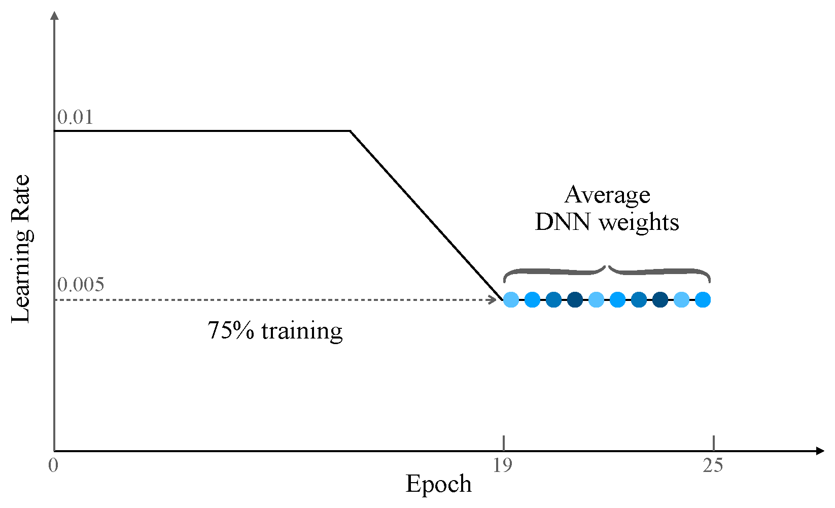
We utilized the PyTorch 2.1 deep learning framework to implement the proposed network. The training and validation were conducted on a server containing four NVIDIA GeForce RTX 3090 GPUs. In our study, we employed a 3D ResNet-18 model that was initially trained on Kinetics-400. We then proceeded to fine-tune this model using the Jester training set. We utilized SGD with a momentum of $0.9$ as the optimizer and conducted training on the model for 25 epochs with a batch size of 16. Following the settings from [15], during the first $75\%$ of training, we adopted the standard decaying learning rate strategy, followed by a consistent and high learning rate for the remaining $25\%$ (as shown in Figure 3). The use of a modified learning rate scheme is expected to keep the optimizer bouncing around the optimum, exploring different models rather than simply converging to a single solution. Our model obtained $90.02\%$ accuracy on the training set at the 25th epoch, with a corresponding cross-entropy loss of approximately $0.28$. At the same time, the validation set achieved its best rate of $86.35\%$ at the 21st epoch.

In addition to evaluating the expected calibration error using ECM, MCE, and RMSCE, we also report the accuracy and average confidence in the model’s classifications. The results obtained from the Jester test dataset are summarized in

Table 1. Summary of classification accuracy, average confidence, RMSCE, MCE, and ECE, compared to other methods, as obtained from the Jester test set. All values are percentages; $(\uparrow )$ indicates that higher values are desirable, $(\downarrow )$ means lower values are better, and bold indicates the best results.

Method	Jester Test Set
	Acc. $(\uparrow )$	Conf. $(\uparrow )$	RMSCE $(\downarrow )$	MCE $(\downarrow )$	ECE $(\downarrow )$
Baseline (SGD)	83.89	87.65	8.73	4.53	3.76
MC-Dropout	84.21	89.91	3.70	8.34	4.83
Logits-Scaling	83.32	87.21	5.19	4.66	4.24
Ours	$\mathbf{84}.\mathbf{44}$	$\mathbf{85}.\mathbf{09}$	3.71	$\mathbf{2}.\mathbf{49}$	$\mathbf{1}.\mathbf{16}$

. We evaluated our method on multiple scoring functions, including SGD (baseline), MC-Dropout [16], and Logits-Scaling [26]. On the Jester test set, our method reduced the ECE error from $3.76\%$ to $1.16\%$. Meanwhile, we observed that our method not only significantly reduced ECE and MCE but also improved the prediction accuracy of the model to a certain extent. For example, classification accuracy increased from $83.89\%$ to $84.44\%$. The experiment report further illustrates the effectiveness of our method in improving the quality of the confidence estimation from DNNs in gesture recognition tasks.

We used visualization to gain an intuitive understanding of the calibration of the predicted probabilities. The reliability diagram illustrates the degree of calibration in the probabilistic predictions of a classifier. The reliability diagram displays the average predicted probability on the x-axis for each bin, while the y-axis reflects the fraction of positive samples, indicating the proportion of samples with positive categories in each bin. The diagram should represent the identity function if the model is accurately calibrated. If the diagonal is not perfect, it suggests the model was not calibrated correctly. The comparison diagrams in Figure 4 show that after using our method, the gap was effectively reduced, and the reliability diagram is closer to an identity function. The upper charts in the figure are visualizations of the average confidence and accuracy, and below them are reliability diagrams.

4.3. Application 2: Image Classification Task

To evaluate the performance of the model in different tasks, we tested our proposed method in an image classification task using the CINIC-10 datasets [27]. They were compiled by combining CIFAR-10 with images selected and downsampled from the ImageNet database. The CINIC-10 datasets had 270,000 images and were divided into three groups for training, validation, and testing. In each subset, there were 10 categories, each with 90,000 images. We used three architectures that were pre-trained on ImageNet for a backbone network (ResNet-50 [28], Wide-ResNet-50 [29], and VGG-16 [30]), and we then fine-tuned them on the CINIC-10 training set using the transfer learning approach. The experimental setup and training strategy are consistent with those presented in Section 4.2.

Comparisons of classification accuracy, average confidence, RMSCE, MCE, and ECE of the different architectures and methods on the CINIC-10 test set are summarized in

Table 2. Summary of classification accuracy, average confidence, RMSCE, MCE, and ECE compared to other methods, as obtained from the CINIC-10 test set, where $(\uparrow )$ indicates higher values are desirable, $(\downarrow )$ means lower values are better, and bold indicates the best result.

Architecture	Method	CINIC-10 Test Set
		Acc. $(\uparrow )$	Conf. $(\uparrow )$	RMSCE $(\downarrow )$	MCE $(\downarrow )$	ECE $(\downarrow )$
ResNet-50	Baseline (SGD)	72.92	75.93	5.22	3.39	3.01
	MC-Dropout	73.03	76.28	5.70	3.62	3.25
	Logits-Scaling	72.46	75.66	6.02	3.59	3.21
	Ours	$\mathbf{73}.\mathbf{63}$	$\mathbf{75}.\mathbf{78}$	$\mathbf{4}.\mathbf{38}$	$\mathbf{2}.\mathbf{80}$	$\mathbf{2}.\mathbf{36}$
Wide-ResNet-50	Baseline (SGD)	73.06	77.01	7.48	4.43	3.97
	MC-Dropout	72.82	77.05	7.85	4.83	4.31
	Logits-Scaling	69.01	72.04	5.67	3.57	3.07
	Ours	$\mathbf{74}.\mathbf{62}$	$\mathbf{76}.\mathbf{38}$	$\mathbf{7}.\mathbf{42}$	$\mathbf{3}.\mathbf{62}$	$\mathbf{2}.\mathbf{52}$
VGG-16	Baseline (SGD)	78.07	82.69	8.95	5.23	4.62
	MC Dropout	78.97	85.23	20.01	7.04	6.29
	Logits-Scaling	76.08	78.42	5.79	2.56	2.37
	Ours	$\mathbf{80}.\mathbf{51}$	$\mathbf{80}.\mathbf{11}$	$\mathbf{3}.\mathbf{56}$	$\mathbf{0}.\mathbf{51}$	$\mathbf{0}.\mathbf{39}$

. We evaluated our method using the same scoring function as in Section 4.2, including: SGD (baseline), MC-Dropout [16], and Logits-Scaling [26]. We observed that the VGG16-based architecture yielded the best confidence calibration, with improved classification accuracy. The other two architectures significantly improved accuracy by about $1.13\%$ on average, compared with the SGD optimization approach. Comparative results demonstrate that our approach decreases the model’s calibration error while also increasing its accuracy.

The MC-dropout method can be viewed as an approximation of Bayesian neural networks. The method requires modification of the original network architecture and in the testing phase. It is also necessary to perform multiple forward propagation and average multiple predictions during the testing phase. In contrast, our method can be regarded as a trainable method. There is no need to modify the model structure, and only one forward propagation is required in the test phase, which greatly reduces the inference time. The Logits-scaling method requires recalculating a hyperparameter T based on the validation set after training and using T to modify the output of softmax during inference on new inputs. An obvious shortcoming of this method is that it is very dependent on data sets and has relatively less generality.

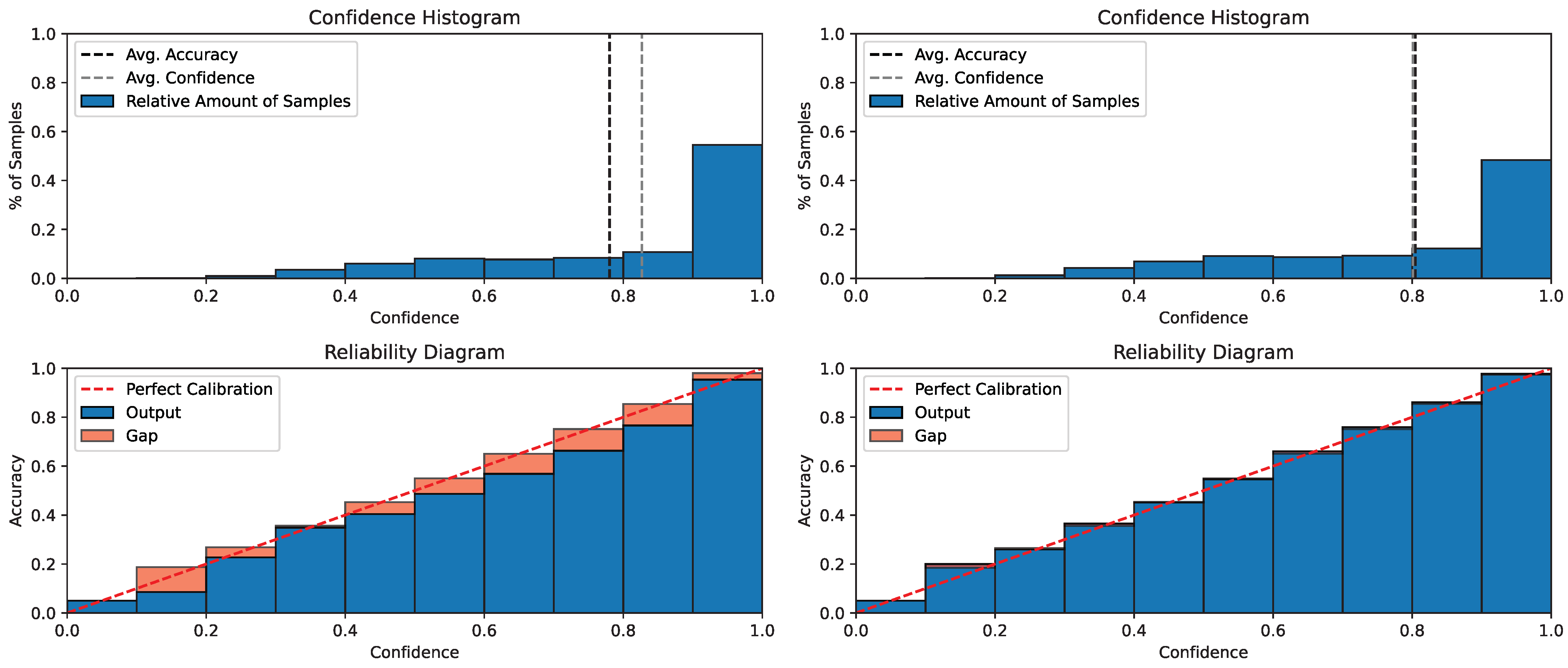
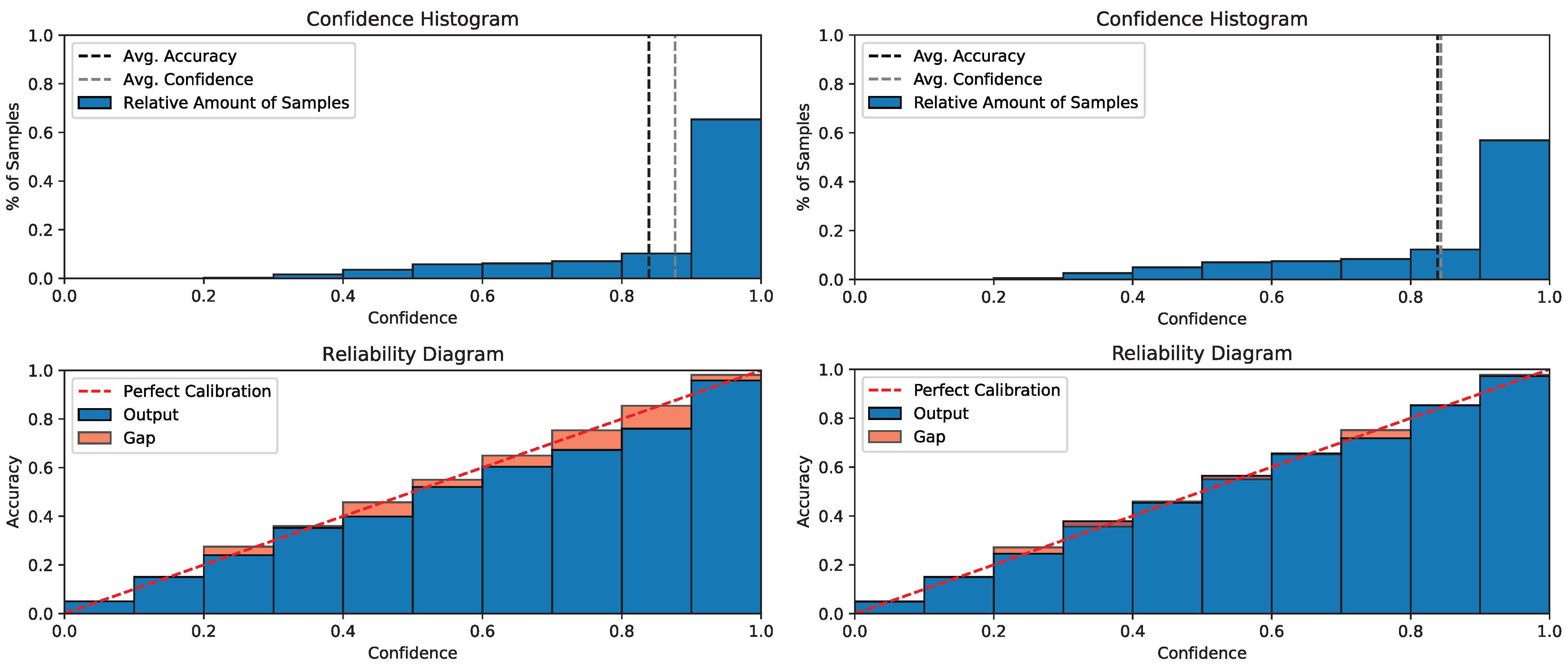
To visualize the calibration effect of our method on the CINIC-10 dataset, we also visualized the calibration curves. The reliability diagram before and after confidence calibration is shown in Figure 5. The red dashed line indicates the best calibration, where the output confidence precisely reflects the accuracy. In the confidence histogram (upper left), we observe a large gap between the mean confidence and the confidence; while in the upper right graph (our method), we can see that this gap is greatly reduced. Comparing the left and right reliability diagrams, we can also visualize that our approach is closer to the red dashed line. These results are consistent with what we observed in application 1 in Section 4.2.

5. Discussion and Future Work

We believe that there are three important factors that make our proposed approach work. First, our method uses a modified learning rate schedule. This allows the optimizer to continuously explore the optimal weights for high performance rather than just reaching or limiting itself to a single solution. For example, we use a standard decaying learning rate strategy for the first 75% of iterations, and a cyclical learning rate for the remaining 25% of iterations. Second, we choose to save the corresponding model weights when the learning rate decays to its lowest value rather then saving model weights according to the validation accuracy. Note that we are using a cyclical learning rate, so the learning rate will decay to the lowest value multiple times; that is, we obtain multiple sets of model weight parameters. The third is to average the model weight parameters traversed by the optimizer. The key idea behind this is to leverage deep learning’s unique training objectives flatness [14] to improve generalization and reduce overconfidence.

DNNs are usually learned through a stochastic training algorithm, which means the DNN is sensitive to the training data and may learn a different set of weights at the end of the training session, resulting in different predictions. The goal of machine learning is to develop methods and algorithms to learn from the data; that is, extract the residing information from the data. In fact, learning parameters from data is an inverse problem; we need to infer the cause (parameters) from the result (observed data). In this work, we proposed an approximate deep ensemble method to calibrate the confidence of DNNs. The ambiguity in target y for a given x was captured by obtaining a probabilistic model with appropriate scoring rules. In addition, the approximate combination of ensembles was used to predict the output for x in an attempt to capture model uncertainty. Through experiments on two benchmark datasets for image classification and gesture recognition, we demonstrated that our method obtained well-calibrated confidence estimates. Removing correlations from individual network predictions to promote ensemble diversity and further improve performance is left to future work. It would be meaningful to refine multiple ensemble models into a simpler single model to obtain a model with good confidence calibration.

References

1. Jiang, X.; Deng, X. Knowledge reverse distillation based confidence calibration for deep neural networks. Neural Process. Lett. 2023, 55, 345–360. [Google Scholar] [CrossRef]
2. Guo, C.; Pleiss, G.; Sun, Y.; Weinberger, K.Q. On calibration of modern neural networks. In Proceedings of the 34th International Conference on Machine Learning, ICML’17, Sydney, NSW, Australia, 6–11 August 2017; pp. 1321–1330. [Google Scholar]
3. Gawlikowski, J.; Tassi, C.R.N.; Ali, M.; Lee, J.; Humt, M.; Feng, J.; Kruspe, A.; Triebel, R.; Jung, P.; Roscher, R.; et al. A survey of uncertainty in deep neural networks. Artif. Intell. Rev. 2023, 56, 1513–1589. [Google Scholar] [CrossRef]
4. Abdar, M.; Pourpanah, F.; Hussain, S.; Rezazadegan, D.; Liu, L.; Ghavamzadeh, M.; Fieguth, P.; Cao, X.; Khosravi, A.; Acharya, U.R.; et al. A review of uncertainty quantification in deep learning: Techniques, applications and challenges. Inf. Fusion. 2021, 76, 243–297. [Google Scholar] [CrossRef]
5. Jospin, L.V.; Laga, H.; Boussaid, F.; Buntine, W.; Bennamoun, M. Hands-on Bayesian neural networks—A tutorial for deep learning users. IEEE Comput. Intell. Mag. 2022, 17, 29–48. [Google Scholar] [CrossRef]
6. Wang, H.; Yeung, D.Y. A survey on Bayesian deep learning. ACM Comput. Surv. 2020, 53, 1–37. [Google Scholar] [CrossRef]
7. Munir, M.A.; Khan, M.H.; Khan, S.; Khan, F.S. Bridging Precision and Confidence: A Train-Time Loss for Calibrating Object Detection. In Proceedings of the Conference on Computer Vision and Pattern Recognition, Los Alamitos, CA, USA, 28 June 2023; pp. 11474–11483. [Google Scholar]
8. Lee, J.; Park, S. A Study on the Calibrated Confidence of Text Classification Using a Variational Bayes. Appl. Sci. 2022, 12, 9007. [Google Scholar] [CrossRef]
9. Psaros, A.F.; Meng, X.; Zou, Z.; Guo, L.; Karniadakis, G.E. Uncertainty quantification in scientific machine learning: Methods, metrics, and comparisons. J. Comput. Phys. 2023, 477, 111902. [Google Scholar] [CrossRef]
10. Ganaie, M.A.; Hu, M.; Malik, A.; Tanveer, M.; Suganthan, P. Ensemble deep learning: A review. Eng. Appl. Artif. Intell. 2022, 115, 105151. [Google Scholar] [CrossRef]
11. Lakshminarayanan, B.; Pritzel, A.; Blundell, C. Simple and scalable predictive uncertainty estimation using deep ensembles. Adv. Neural Inf. Process. Syst. 2017, 30, 1–12. [Google Scholar]
12. Ovadia, Y.; Fertig, E.; Ren, J.; Nado, Z.; Sculley, D.; Nowozin, S.; Dillon, J.; Lakshminarayanan, B.; Snoek, J. Can you trust your model’s uncertainty? evaluating predictive uncertainty under dataset shift. Adv. Neural Inf. Process. Syst. 2019, 32, 1–12. [Google Scholar]
13. Huang, G.; Li, Y.; Pleiss, G.; Liu, Z.; Hopcroft, J.E.; Weinberger, K.Q. Snapshot Ensembles: Train 1, get M for free. arXiv 2017, arXiv:1704.00109. [Google Scholar]
14. Garipov, T.; Izmailov, P.; Podoprikhin, D.; Vetrov, D.P.; Wilson, A.G. Loss surfaces, mode connectivity, and fast ensembling of dnns. Adv. Neural Inf. Process. Syst. 2018, 31, 1–10. [Google Scholar]
15. Izmailov, P.; Podoprikhin, D.; Garipov, T.; Vetrov, D.P.; Wilson, A.G. Averaging Weights Leads to Wider Optima and Better Generalization. In Proceedings of the Conference on Uncertainty in Artificial Intelligence, Monterey, CA, USA, 6–10 August 2018. [Google Scholar]
16. Gal, Y.; Ghahramani, Z. Dropout as a bayesian approximation: Representing model uncertainty in deep learning. In Proceedings of the International Conference on Machine Learning, New York, NY, USA, 19–24 June 2016; pp. 1050–1059. [Google Scholar]
17. Mller, R.; Kornblith, S.; Hinton, G.E. When does label smoothing help? Adv. Neural Inf. Process. Syst. 2019, 32, 1–10. [Google Scholar]
18. Rahaman, R. Uncertainty quantification and deep ensembles. Adv. Neural Inf. Process. Syst. 2021, 34, 20063–20075. [Google Scholar]
19. Patel, K.; Beluch, W.; Zhang, D.; Pfeiffer, M.; Yang, B. On-manifold adversarial data augmentation improves uncertainty calibration. In Proceedings of the 25th International Conference on Pattern Recognition, Milan, Italy, 10–15 January 2021; pp. 8029–8036. [Google Scholar]
20. Yang, Y.; Lv, H.; Chen, N. A survey on ensemble learning under the era of deep learning. Artif. Intell. Rev. 2023, 56, 5545–5589. [Google Scholar] [CrossRef]
21. Mienye, I.D.; Sun, Y. A survey of ensemble learning: Concepts, algorithms, applications, and prospects. IEEE Access 2022, 10, 99129–99149. [Google Scholar] [CrossRef]
22. Mahajan, P.; Uddin, S.; Hajati, F.; Moni, M.A. Ensemble Learning for Disease Prediction: A Review. Healthcare 2023, 11, 1808. [Google Scholar] [CrossRef]
23. Guo, H.; Liu, H.; Li, R.; Wu, C.; Guo, Y.; Xu, M. Margin diversity based ordering ensemble pruning. Neurocomputing 2018, 275, 237–246. [Google Scholar] [CrossRef]
24. Fernando, K.R.M.; Tsokos, C.P. Dynamically weighted balanced loss: Class imbalanced learning and confidence calibration of deep neural networks. IEEE Trans. Neural Netw. Learn. Syst. 2021, 33, 2940–2951. [Google Scholar] [CrossRef]
25. Materzynska, J.; Berger, G.; Bax, I.; Memisevic, R. The Jester Dataset: A Large-Scale Video Dataset of Human Gestures. In Proceedings of the 2019 International Conference on Computer Vision Workshop, Seoul, Republic of Korea, 27 October–2 November 2019; pp. 2874–2882. [Google Scholar]
26. Wei, H.; Xie, R.; Cheng, H.; Feng, L.; An, B.; Li, Y. Mitigating neural network overconfidence with logit normalization. In Proceedings of the International Conference on Machine Learning, Baltimore, MD, USA, 17–23 July 2022; pp. 23631–23644. [Google Scholar]
27. Darlow, L.N.; Crowley, E.J.; Antoniou, A.; Storkey, A.J. Cinic-10 is not imagenet or cifar-10. arXiv 2018, arXiv:1810.03505. [Google Scholar]
28. He, K.; Zhang, X.; Ren, S.; Sun, J. Deep residual learning for image recognition. In Proceedings of the Conference on Computer Vision and Pattern Recognition, Las Vegas, NV, USA, 27–30 June 2016; pp. 770–778. [Google Scholar]
29. Zagoruyko, S.; Komodakis, N. Wide residual networks. arXiv 2016, arXiv:1605.07146. [Google Scholar]
30. Simonyan, K.; Zisserman, A. Very deep convolutional networks for large-scale image recognition. arXiv 2014, arXiv:1409.1556. [Google Scholar]
Figure 1. Illustration of the 3D loss landscape with SGD optimization of the DNN during the training phase.
Electronics 13 00503 g001
Figure 2. The data flow of fusion during the testing phase of our method, where  θ 1 , θ 2 , , θ m  indicate the set of m base estimators, and  y ^  represents the output of base estimator,  θ m , on sample x.
Electronics 13 00503 g002
Figure 3. Illustration of the learning rate schedule. During the initial  75 %  of training, a standard decaying schedule is employed, followed by a high constant value for the remaining  25 % . The dots of different colors represent the weights of the model in different training epochs.
Electronics 13 00503 g003
Figure 4. Comparison of reliability diagram and confidence histogram on the Jester test set. The upper charts are visualizations of average confidence and accuracy, and below them are reliability diagrams from (left) the SGD optimization method and (right) from our method.
Electronics 13 00503 g004
Figure 5. Comparison of reliability diagram and confidence histogram from VGG-16 trained on the CINIC-10 test set. The upper charts are visualizations of average confidence and accuracy, and below them are reliability diagrams from (left) the SGD optimization method and (right) from our method.
Electronics 13 00503 g005