A Lightweight 6D Pose Estimation Network Based on Improved Atrous Spatial Pyramid Pooling

Abstract

It is difficult for lightweight neural networks to produce accurate 6DoF pose estimation effects due to their accuracy being affected by scale changes. To solve this problem, we propose a method with good performance and robustness based on previous research. The enhanced PVNet-based method uses depth-wise convolution to build a lightweight network. In addition, coordinate attention and atrous spatial pyramid pooling are used to ensure accuracy and robustness. This method effectively reduces the network size and computational complexity and is a lightweight 6DoF pose estimation method based on monocular RGB images. Experiments on public datasets and self-built datasets show that the average ADD(-S) estimation accuracy and 2D projection index of the improved method are improved. For datasets with large changes in object scale, the estimation accuracy of the average ADD(-S) is greatly improved.

1. Introduction

In today’s quest for intelligence-driven technology, applications such as intelligent car driving, augmented reality, human–computer interactions, etc., are gradually transitioning from concepts to real life. The realization of all these applications relies heavily on support from relevant technologies. Six-degree-of-freedom (6D) object pose estimation based on computer vision is an important technology in this regard. The key to this technology lies in recovering the 3D translation and 3D rotation information of target objects from images or point cloud data. Accurately and efficiently estimating the 6D information of objects in real-world scenarios is of significant value for enhancing the safety of automated driving, strengthening the immersion of virtual and real interactions, and improving the reliability of robotic operations.

Unlike traditional 6D pose estimation methods that rely on multiple sensors, computer vision-based methods are currently the mainstream approach in research, significantly reducing the complexity and application costs of the entire pose estimation system. Early methods based on template matching involve the construction of a template library of the same target object from images at different angles and distances, calculating the similarity between the real value and template images in the estimation task. However, such methods are computationally complex and time-consuming. Subsequently, algorithms like SIFT [1], FAST [2], and BRIEF [3] have been applied to extract invariant features from images as key points, with pose estimation then being performed by matching key points with real points. However, objects in real environments are often affected by factors such as complex backgrounds, changes in lighting conditions, occlusions, and variations in viewpoints, leading to difficulties in extracting effective key points. With the development of 3D scanning technology, the difficulty of obtaining 3D object models has been reduced. Methods based on aligning models with object images or point clouds have been proposed, which offer high pose estimation accuracy. However, these methods require high model accuracy, depend on depth information, and have poor applicability to non-rigid objects [3].

With the successful application of deep learning methods in various tasks, researchers have begun to explore the use of deep neural networks (DNNs) to solve the 6D pose estimation problem for RGB images. As a pioneering work, PoseNet [4] was the first to adopt a CNN to regress camera pose from a single image, successfully proving that it is possible to achieve end-to-end camera pose regression with just one picture as input [5]. Deep learning methods, such as CNNs, can automatically learn feature representations, making the extracted key points more robust, effectively capturing the structure and semantic information of images and thus enhancing feature discrimination. In particular, in complex scenarios common in object pose estimation, such as cluttered backgrounds, changes in lighting, and object occlusion, deep learning-based pose estimation methods have achieved promising results. Researchers designing conventional 6D pose estimation methods tend to focus more on designing complex networks to improve estimation performance while ignoring the practical deployment challenges arising from the high model complexity and large parameter counts.

To address this issue and meet the needs of typical applications like mobile augmented reality, in this paper, a lightweight, deep learning-based pose estimation method is proposed. By improving the pose estimation network and using RGB images obtained from monocular cameras to estimate the six-degree-of-freedom camera pose, the method achieves robustness and accuracy while meeting the requirements for lightweight deployment. The main contributions of this paper are as follows:

• To reduce the computational cost of 6D object pose estimation, we propose a lightweight model in which residual depth-wise separable convolution is combined with an improved atrous spatial pyramid pooling (ASPP) method.
• We introduce a coordinate attention mechanism and address the issue of object scale variation, which was not considered in the original method. Additionally, we incorporate a multi-scale pyramid pooling module. These enhancements effectively reduce the model’s parameter and computation complexity while significantly improving the pose estimation accuracy for objects with large-scale variations.
• The effectiveness of this lightweight model is validated and analyzed through experiments on both publicly available and self-built datasets.

2. Related Works

DNNs learn object poses directly from images or point cloud data, reducing the reliance on depth information typical in traditional methods and thus driving the rapid development of pose estimation methods based on monocular RGB images. Deep learning 6D pose estimation methods can be classified into two categories based on the training strategy: direct strategy and indirect strategy methods.

Deep learning methods based on a direct strategy are also known as single-stage methods. In this approach, depth information is combined and the embedding space of poses is learned directly, or 3D translation and rotation information is regressed directly, through end-to-end learning. Its mapping relationship is simple and it has a fast inference speed. To address the limited accuracy of directly regressing pose estimation from images, the DeepIM model optimizes poses by iteratively training CNNs to match model-rendered images with input images [6]. In scenes with occlusions and clutter, in Posecnn, translation information is estimated by locating objects in the center of the image relative to the camera distance, and object rotation is estimated through regression representation, which is capable of handling symmetric objects [7]. This network can simultaneously perform both object detection and pose estimation tasks. Wang et al. [8] designed the DenseFusion framework for RGB-D datasets, which fully utilizes integrated complementary pixel information and depth information for pose estimation and integrates an end-to-end iterative pose optimization program, achieving real-time inference. YOLO-based methods have an advantage in pose estimation compared to other methods with regard to processing speed and are more advantageous for real-time estimations [9,10]. Single-stage deep learning methods can simultaneously complete object pose estimation in one stage with faster inference speeds, making them more applicable to applications with high real-time requirements. However, they may have slight shortcomings regarding accuracy and robustness.

In deep learning-based pose estimation methods relying on the indirect strategy, 6D pose estimation tasks are primarily completed using single-view RGB images. This method is also known as the two-stage approach, where the entire task flow is divided into two stages: establishing 2D–3D correspondence relationships for key points and recovering pose information using PnP/RANSAC variant algorithms. Compared to direct strategy methods, it has advantages with regard to robustness and accuracy when occlusions, lighting changes, or complex backgrounds are present. Visual occlusion is a common problem in practical applications. To address this, Rad et al. proposed the BB8 method, which uses a convolutional neural network to estimate a pose by locating the spatial positions of eight corner points of the object, which showed good robustness against occlusion and cluttered backgrounds [11]. Zhao et al. [12] further selected key points from eight corner points in space. This was improved upon in PVNet, where sparse key points are discarded as reference points, pixel-to-key point vectors are introduced through a semantic segmentation network, and the estimation accuracy is enhanced in scenarios with occlusion and symmetric objects [13]. Pix2Pose utilizes adversarial generative networks to address similar issues [14]. Chen et al. proposed a method that first calibrates in two dimensions and then estimates poses using 2D–3D correspondence relationships, achieving significant breakthroughs in accuracy [15].

In summary, indirect strategy methods have advantages with regard to robustness and accuracy in complex environments, but they involve more steps and require more computational resources and time.

3. Improved Model Based on Atrous Spatial Pyramid Pooling

To reduce the computational cost of object 6D pose estimation, in this paper, a lightweight model is proposed, combining residual depth-wise separable convolution with an improved ASPP method based on PVNet. Firstly, we utilized residual depth-wise separable convolution layers to construct a lightweight network, thereby reducing the demand for memory and computing resources. Secondly, to prevent the loss of channel and coordinate information caused by multi-layer convolutions, which affects the estimation accuracy, we introduced a coordinate attention mechanism. Addressing the issue of inadequate recognition accuracy in previous methods caused by neglecting object scale changes, we added a multi-scale pyramid pooling module for processing. Finally, a two-stage pixel voting and PnP (Perspective-n-Point) solving task was performed on the decoder’s output feature maps. This approach effectively reduced the model’s parameter and computational overhead, resulting in a significant improvement in the pose estimation accuracy for objects with large-scale variations. The complete 6D pose estimation network framework is illustrated in Figure 1.

3.1. Backbone Network

The backbone network based on improved ASPP consists of 13 layers of depth-wise separable convolution, a coordinate attention mechanism module, and an ASPP module as the encoder, followed by three upsampling and convolution operations in the decoder. The final output is a target segmentation feature map. The network architecture is illustrated in Figure 2.

3.1.1. Residual Depth-Wise Separable Network

In PVNet, outstanding performance in keypoint detection is achieved by using a pre-trained ResNet model based on a large-scale dataset as the target segmentation network, leading to a significant improvement in the accuracy of 6D pose estimation over previous methods [16]. However, this model and its related improvements have a relatively large volume, making them difficult to deploy on devices with requirements for lightweight applications. Drawing inspiration from the MobileNet series of algorithms [17,18], in this study, a lightweight backbone network model based on depth separable convolution operations was designed, significantly reducing the number of network layers and model parameters.

The depth separable convolution operation can be seen as the process of splitting a standard convolution into a grouped convolution and a pointwise convolution. Compared to standard convolution, which convolves an image with m channels using n sets of corresponding m × 3 × 3 convolution kernels to generate n feature maps, in-depth separable convolution, a two-stage mode, was adopted. First, a 1 × 3 × 3 convolution kernel was applied to each of the m channels, generating m intermediate feature maps, and then n sets of m × 1 × 1 convolution kernels were used to generate n feature maps. Figure 3 illustrates the process of the two convolutions.

Aiming to produce a feature map with C_oup channels using a square convolution kernel of size k × k, following a uniform standard where bias parameters with a quantity of 1 are disregarded and each multiply–add operation is treated as one floating-point calculation, for an input image with dimensions of W × H and C_inp channels, we can approximate the parameter and computation complexity of standard convolution as follows:

$$Paramsstd=Coup\times k_2\times Cinp$$

(1)

$$FLOPsstd=Cinp\times k_2\times Coup\times W\times H$$

(2)

An approximate description of the parameter and computation complexity of depth-wise separable convolution is as follows:

$$Paramsdw\&pw=Cinp\times k_2+1\times Cinp\times Coup$$

(3)

$$FLOPsdw\&pw=Cinp\times k_2\times W\times H+1\times Cinp\times Coup\times W\times H$$

(4)

Compared to standard convolution operations, the parameter and computation complexity required for depth-wise separable convolution is $\frac{1}{Coup}+\frac{1}{k^2}$ times that of standard convolution. Particularly in this model, where the output channels of the image ranged from 64 to 1024 and the depth-wise separable convolution kernels were all 3 × 3 in size, there was a significant advantage in reducing the computational overhead compared to standard convolution. Considering that, in the process of semantic segmentation, multiple downsampling and convolution operations on the original image may lead to the loss of low-dimensional information, adding residual connections to convolution layers with the same input and output channels preserves low-dimensional feature information while obtaining high-dimensional semantic information after convolution, which significantly improves the final accuracy of object pose estimation.

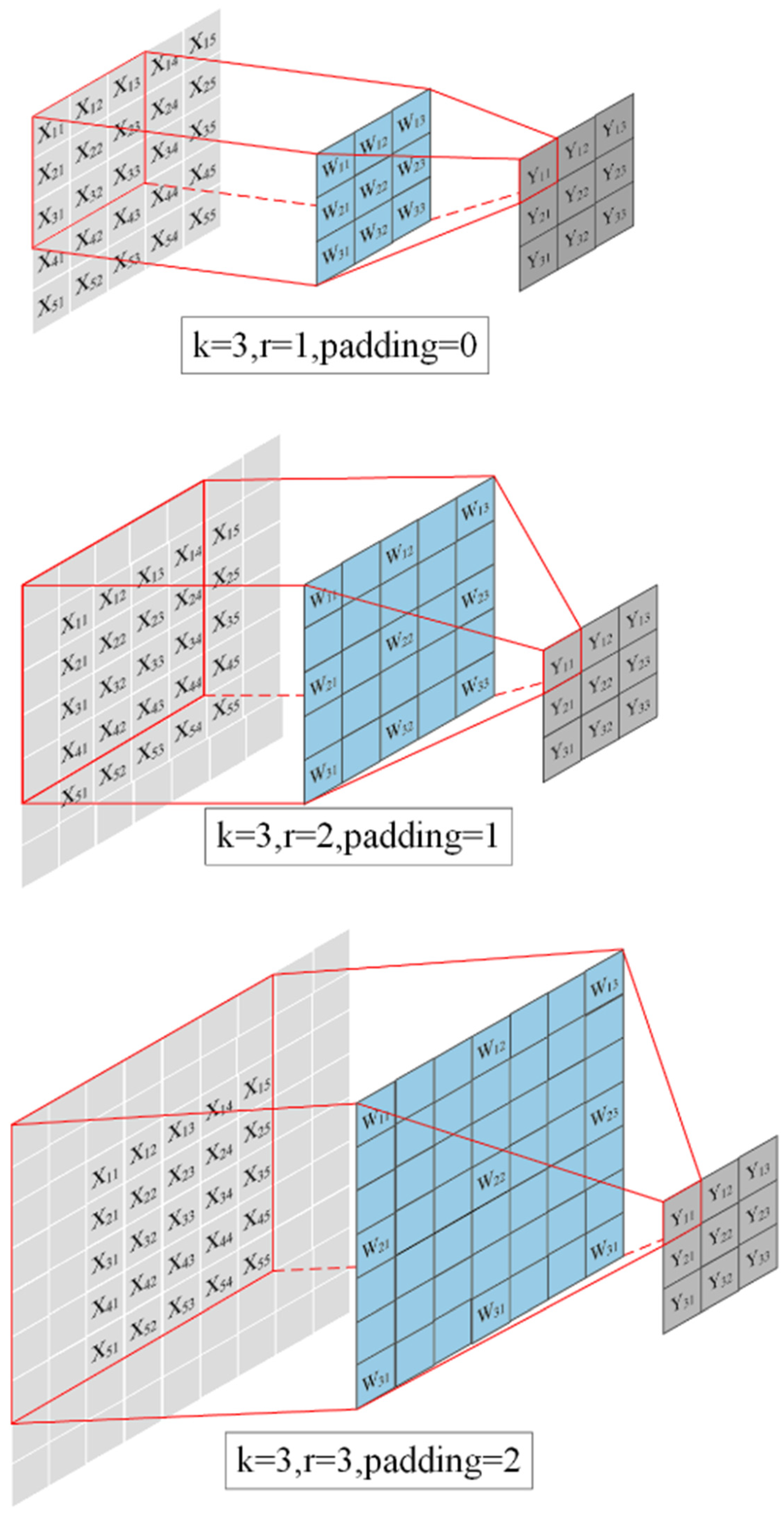
3.1.2. Improved Atrous Spatial Pyramid Pooling

In the decoder part of the network, feature extraction was performed through convolution and pooling operations. All output feature maps were compressed into a single feature vector via global average pooling, which ignored the non-uniformity of features across different channels. Additionally, influenced by the number of layers and the size of convolution kernels, lightweight networks often overlook the spatial positional information of features.

The coordinate attention mechanism [19] is an attention method suitable for lightweight networks. It is characterized by a lightweight and plug-and-play nature and can capture inter-channel information while also considering directional and positional information. Additionally, it achieves significant improvement in tasks such as object detection and semantic segmentation, which involve dense predictions. In the coordinate attention mechanism, average pooling and concatenation were performed in both the horizontal and vertical directions and channel information was fused through convolution, encoding spatial information simultaneously. After splitting, multiplication with the input features was performed, emphasizing feature information in spatial positions. The coordinate attention mechanism notably enhanced the performance of dense prediction tasks in lightweight mobile networks. Through experimental analysis, it was decided to place it at the end of the encoder, reducing interference from subsequent convolution operations. Additionally, the reduced number of channels at the end could decrease computational costs.

The application of depth-wise separable convolution significantly reduced the model complexity. However, in computer vision-related tasks, the size of the receptive field largely determines the effectiveness of the model. Increasing the network depth and using larger convolutional kernels are direct and effective methods to enhance the receptive field. However, they inevitably exacerbate model complexity. Through experiments, it has been found that simply increasing the network depth results in limited performance improvements relative to the cost incurred.

Luo et al. [20] proposed the concept of an effective receptive field, demonstrating in their work that the effective receptive field only represents a portion of the entire receptive field. Therefore, a larger receptive field is needed in practice to cover the desired region. Dilated convolution, also known as atrous convolution, is one method to effectively enlarge the receptive field. This is achieved by introducing “holes” into the convolutional kernel, effectively expanding the receptive field without increasing the number of parameters in the kernel.

The ASPP module extends the concept of dilated convolution by introducing multiple dilated convolutions with different rates [21]. It considers feature information from multiple receptive fields, thereby enhancing the perception of objects at different scales. Figure 4 illustrates dilated convolutions with different rates. By employing this method, it is possible to capture object boundaries and detailed information while reducing computational complexity, thereby improving the recognition accuracy.

Building upon ASPP, an attention mechanism module was incorporated to further enhance the feature information at different scales, highlighting key point information. Given the limited overall data volume of single-target training samples, overfitting was likely to occur. Therefore, a dropout layer was applied at the output end during training. During the forward propagation process, random hidden neurons were dropped, reducing the interdependency between neurons and enhancing the network’s generalization capability. The mathematical expression for dropout is expressed as follows:

$$y_i=\left\{ \begin{array}{c}0, dropout\left(probability=p\right),\\ \frac{x_i}{1-p}, otherwise. \end{array} \right.$$

(5)

where $y_i$ and $x_i$ represent the output and input of neuron $i$, respectively. During training, the output was zeroed out with probability p; during testing, dropout was not applied.

For tasks requiring dynamic object pose estimation, scale variation poses a significant challenge. Compared to previous work, the improved ASPP module exhibits a noticeable robustness enhancement in pose estimation accuracy for datasets with significant scale variations. The improved ASPP module is illustrated in Figure 5.

3.2. Pixel Voting and Pose Estimation

The input RGB image underwent a target segmentation task through a pre-trained backbone network, obtaining the segmented object image as an output. Between the 2D key point x on the segmented image and any pixel point p, there existed a unit vector $vx\left(p\right)$, satisfying the relation $vx\left(p\right)=\frac{x-p}{{\left|\left|x-p\right|\right|}_2}.$ Two pixel points on the image were randomly selected, and the intersection of the unit vectors pointing to the possible positions of the key point was taken as the hypothesis position $h_1$. This process was repeated n times to generate a set of n hypotheses $\left\{hi\right|i=1, . . . , n\}$. For $p\in O$ (a pixel point p belonging to the target 0), there existed a corresponding vector $vh\left(p\right)=\frac{h_i-p}{{\left|\left|h_i-p\right|\right|}_2}$ for each hypothesis. Whether a hypothesis was assigned depended on whether the dot product $v=vx\left(p\right)·vh\left(p\right)$ met the threshold $\theta$ of the indicator function $1\theta \left(v\right)$. This step is referred to as pixel voting. After completing the pixel voting process, the voting score of this set of hypotheses needed to be consistent with the spatial distribution of the true key points. Therefore, the hypothesis point with the highest score was considered the most likely to be the true key point. The scoring function and the calculation formula for the i-th hypothesis are as follows:

$$1\theta \left(v\right)=\left\{\begin{array}{c}1, if v>\theta ,\\ 0, otherwise. \end{array} \right.$$

(6)

$$wi={\sum }_{p\in O}1\theta \left(v\right)$$

(7)

After completing the scoring calculation for n hypotheses, the position information of the hypothesis with the highest score was selected as the position information for the true key point. Through the approximate random consensus sampling method, pixels belonging to the target were randomly selected, thus maintaining the uniformity of the pixel distribution involved in voting and reducing unnecessary score calculations.

The rotation matrix R is a 3 × 3 matrix used to describe the rotational changes of an object in three-dimensional space. It is a common representation method for describing rotations in 3D space. Each column of the matrix typically represented the rotations of the object around the X, Y, and Z axes of the coordinate system, respectively. This method provided a transformation representation from one coordinate system to another, where each column vector represented the direction of a coordinate axis in the rotated coordinate system relative to the original coordinate system.

The translation matrix T was a 3 × 1 vector that described the displacement or shift of an object in three-dimensional space. This vector extended the object’s position from its original location to a new location within the coordinate system.

Unlike Euler angles, the rotation matrix representation method does not suffer from gimbal lock issues and provides a continuous and unique representation throughout the entire rotation space. This means that rotation matrices can represent arbitrary rotations without being limited by specific axis orders or rotation sequences, offering a more flexible and stable representation of rotations.

$$R\left[\begin{array}{ccc}{r}_{11}& r_{12}& r_{13}\\ r_{21}& r_{22}& r_{23}\\ r_{31}& r_{32}& r_{33}\end{array}\right]$$

(8)

$$[R|T]\left[\begin{array}{ccc}{r}_{11}& r_{12}& r_{13} \\ r_{21}& r_{22}& r_{23} \\ r_{31}& r_{32}& r_{33}\end{array}\begin{array}{c} x\\ y\\ z\end{array}\right]$$

(9)

By calculating the coordinates of key points through pixel voting and utilizing the rotation matrix representation method, combined with the 3D object model, the pose information of the object could be estimated.

The data obtained by projecting the known 3D model of the target object into two dimensions and annotating the key points were input into the neural network for training to obtain the spatial mapping from 3D to 2D, enabling the neural network to predict key points. Subsequently, the PnP algorithm or trained network inferred the 3D point location information based on the 2D key points. That is, given an RGB image I and a set of corresponding key point information, consisting of 2D key point information of the image $O=\left\{Oi\right|i=1,...,N\}$ and 3D model point information of the object $M=\left\{Mi|i=1,...,N\right\},$ we aimed to solve the pose relationship $P=\left[R\right|T]$.

The method of pixel voting improved the issue of key point selection on objects in 2D images. The selection of actual points on the object in 3D models also impacts the solution results. By employing furthest-point sampling, the 3D model’s surface points were sampled as key points, resulting in a uniform key point distribution across the 3D model’s surface. Experiments on PVNet have demonstrated that this method effectively reduces interference compared to traditional methods relying on corner points as key points, thereby enhancing the pose estimation accuracy.

3.3. Training Strategy

Monocular RGB images were used as training and testing samples. In the 6D object pose estimation task, typically, 15% of the data were chosen as training samples and 85% were chosen as testing samples. The model was trained for 120 epochs on the entire dataset, with an initial learning rate of 4 × 10⁻³. After every 20 epochs, the learning rate was reduced by half.

The output target segmentation image was treated as a binary classification problem, where the task was to determine whether an object was in the foreground (object) or background (interference). The cross-entropy loss function was used as the main loss function for the backbone network. The distance between generated hypothesis points and true key points could intuitively infer the error of the result. This was equivalent to the squared sum of the horizontal and vertical components of the vector difference, $\mathsf{\Delta }vk\left(p\right)=\widetilde{vk\left(p\right)}-vk\left(p\right)$, pointing from any pixel to the hypothesis and true points. To address the issue of outlier gradient explosions, smooth L1 Loss was employed to smooth outliers, and the sum of losses for all key points was used as the loss function for key point prediction.

$$Loss={\sum }_{k=1}^K(s\_L1({\mathsf{\Delta }vk\left(p\right)}_x+s_{L1\left({\mathsf{\Delta }vk\left(p\right)}_y\right)}$$

(10)

$$Loss\left(abs\right)={\sum }_{k=1}^K(\left|{\mathsf{\Delta }vk\left(p\right)}_x\right|+|{\mathsf{\Delta }vk\left(p\right)}_y|)$$

(11)

The same loss function results can be caused by position offsets and scale differences. To reduce interference caused by scale changes, the distance from the hypothesis points to the center point was added as a reference. The absolute value of the sum of $\mathsf{\Delta }vk\left(p\right)$ in the horizontal and vertical directions, denoted as Loss(abs), was used as a reference; under the same loss condition, the smaller the Loss(abs), the greater the scale change.

4. Experimental Results and Analysis

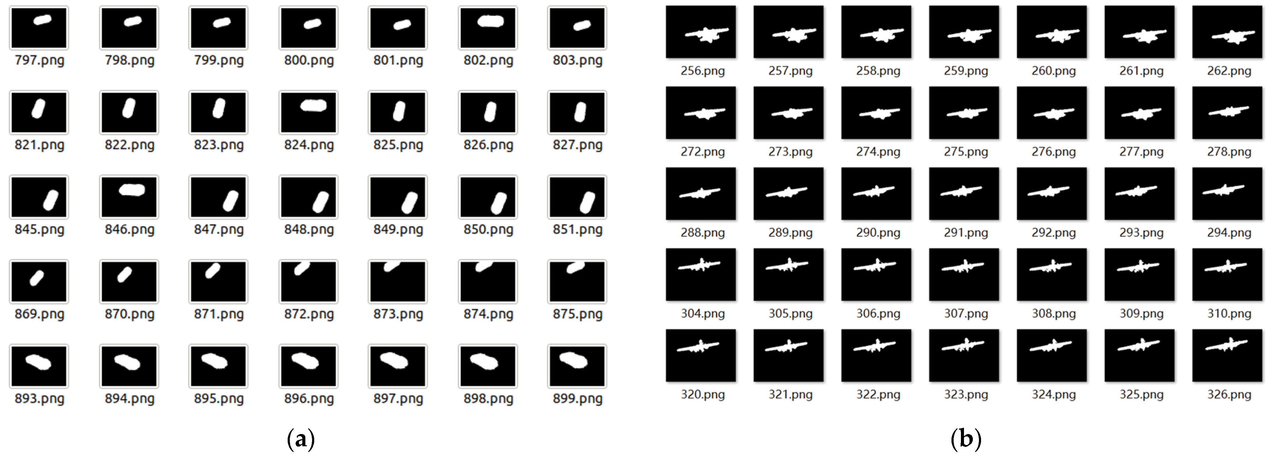
4.1. Dataset

Commonly used datasets for 6D object pose estimation include LineMOD, LineMod-Occlusion [22], and T-LESS [23]. The LineMOD dataset contains RGB-D image data and corresponding labels for multiple small geometric objects with complex shapes, countering challenges such as weak object texture features, complex background environments, and varying lighting conditions. In this study, we not only conducted pose estimation tests on the LineMOD dataset but also designed new datasets using 3D cameras, including an airplane model dataset and a car model dataset, to determine the accuracy improvements of our method for multi-type, multi-scale object pose estimation. These two datasets also present various challenges, including significant scale changes, weak texture features, blurry images, lighting variations, and incomplete objects.

The assembly of the self-built datasets followed the production process used for the LineMOD dataset. Images of objects were captured from various angles in various poses under different lighting conditions using an RGB-D camera (Realsense2). This process yielded RGB images, depth images, and intrinsic camera parameter data for the objects. Aruco markers in the images were used for registration between pairs of images, and the matrix transformation between two sets of points was calculated. Through iterative registration and optimization, a globally consistent transformation was generated, producing pose change files (4 × 4 homogeneous matrices) for each image relative to the first frame. The depth image data were converted into point clouds and denoised. Meshlab, a mesh processing tool, was used to remove unwanted scene content, as shown in Figure 6. Finally, based on the pose changes and processed mesh, relocalization was performed to compute the 2D projection information of the new mesh in the camera’s coordinates. Corresponding pixel masks (Figure 7) and label files representing the true pose information were generated.

In the experiments, RGB images were used for training and testing, while depth images were used to obtain point cloud data to reconstruct 3D models. It should be noted that there may have been some differences in label accuracy between the self-built dataset and the LineMOD dataset, which may have resulted in the 2D projection performance being inferior for the self-built dataset compared to the LineMOD dataset in terms of precision.

4.2. Performance Evaluation Metrics

ADD and ADD-S, respectively, represent the average distance of points and the average distance of the nearest points, and are the most used evaluation metrics for rigid object pose estimation. ADD measures accuracy by computing the average distance between the 3D model points predicted by the pose estimation algorithm and the corresponding annotated model points. ADD-S extends ADD by considering symmetric objects and calculates distances based on the nearest point criterion for symmetric objects. The errors in translation and rotation for ADD(-S) metrics depend on the size and shape of the rigid body, and a threshold of 10% is typically set on the model’s diameter. The 2D projection performance metric measures algorithm accuracy by projecting the model vertices of the target object onto the 2D image plane and computing the average error between the 2D projection points predicted by the pose estimation algorithm and the true annotated 2D vertices. In this paper, we primarily use these two metrics to evaluate the performance of our method.

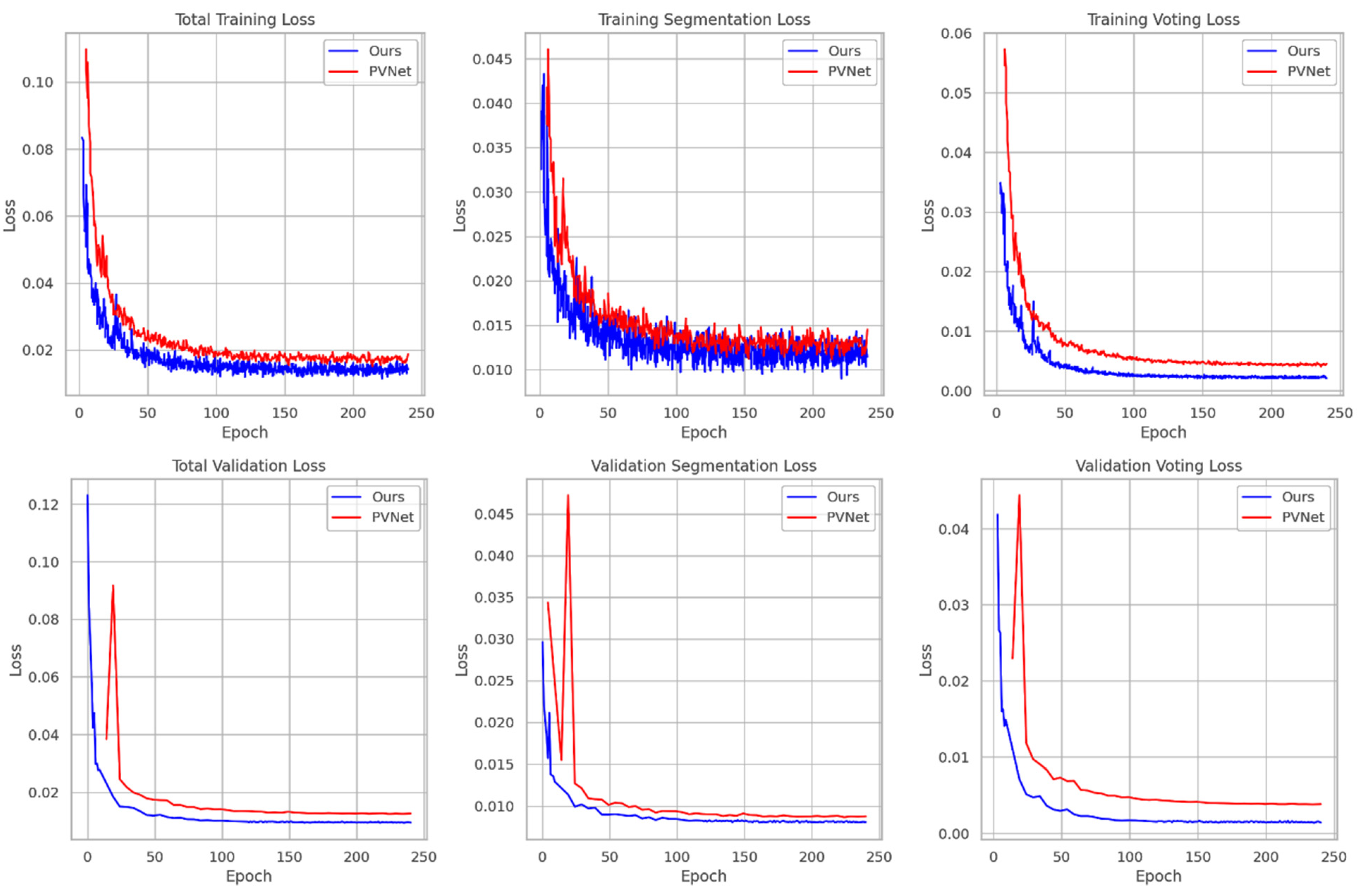
4.3. Experimental Results

The experiments were performed on the Ubuntu 18.04 operating system utilizing the Torch 1.8 deep learning framework with CUDA version 11.1. In terms of hardware, an Intel(R) Xeon(R) Platinum 8255C twelve-core processor was employed as the CPU, while an RTX 3090 GPU was used. The performance of the improved method and baseline method was quantitatively determined on the LineMOD dataset in terms of the ADD(-S) and 2D projection metrics, respectively, as shown in

Table 1. The ADD(-S) accuracy of our method and the baseline method for the LineMOD dataset and the self-built dataset. The middle column represents the pose estimation accuracy without refinement processing, while the right column represents the pose estimation accuracy after refinement processing. Datasets labeled with a superscript “+” indicate symmetric object datasets.

	Without Refinement					Refinement
Method	Zhao	PVNet	DPOD [24]	SSPE [25]	Ours	DPOD+	RePose [26]
Ape	41.2	43.62	53.28	52.5	67.05	87.70	79.5
Benchvice	85.7	99.90	95.34	-	98.46	98.50	100.0
Cam	78.9	86.86	90.36	-	88.24	96.10	99.2
Can	85.2	95.47	94.10	99.2	97.65	99.70	99.8
Cat	73.9	79.34	60.38	88.5	85.86	94.70	97.9
Driller	77.0	96.43	97.72	98.8	93.66	98.80	99.0
Duck	42.7	52.58	66.01	68.7	75.24	86.30	80.3
Eggbox +	78.9	99.15	99.72	100.0	99.72	99.90	100
Glue +	72.5	95.66	93.83	98.5	75.86	96.80	98.3
Hole puncher	63.9	81.92	65.83	88.1	79.46	86.90	96.9
Iron	94.4	98.88	99.80	-	95.23	100.0	100.0
Lamp	98.1	99.33	88.11	-	98.85	96.80	99.8
Phone	51.0	92.41	74.24	-	87.90	94.70	98.9
Aircraft	-	71.72	-	-	79.80	-	-
Car	-	83.17	-	-	97.34	-	-
Average	72.6	85.09	82.98	86.8	88.02	95.15	96.1

and

Table 2. The 2D projection performance accuracy of our method and the baseline method for the LineMOD dataset. Datasets labeled with a superscript “+” indicate symmetric object datasets.

	BB8	YOLO-6D	PVNet	Ours
Ape	95.3	92.10	99.23	100.0
Bench vice	80.0	95.06	99.81	99.52
Cam	80.9	93.24	99.21	99.22
Jar	84.1	97.44	99.90	99.90
Cat	97.0	97.41	99.30	99.60
Driller	74.1	79.41	96.92	98.82
Duck	81.2	94.65	98.02	99.05
Eggbox +	87.9	90.33	99.34	98.87
Glue +	89.0	96.53	98.45	98.85
Hole puncher	90.5	92.86	100.0	99.62
Iron	78.9	82.94	99.18	98.98
Lamp	74.4	76.87	98.27	97.70
Phone	77.6	86.07	99.42	99.52
Average	83.9	90.37	99.00	99.20

.

In the experiments on the LineMOD dataset, our proposed method outperformed most of the baseline methods in terms of the average ADD(-S) accuracy, with an average improvement of 1.93% compared to PVNet. Particularly, there was a significant improvement in pose recognition for objects with relatively large-scale variations, such as apes, cans, and ducks, with the maximum improvement reaching 13.04%. For the self-built dataset with lower precision and lower general image quality, the recognition accuracy of the proposed method was relatively superior, demonstrating better robustness for practical applications. Similarly, the self-built datasets of airplanes and car models also exhibited relatively large variations in object scale, indicating the excellent performance of our method in pose estimation for objects with significant scale changes. As shown in Table 2, the proposed method outperformed the baseline method in terms of the 2D projection performance accuracy. However, considering the correlation heatmap between the 2D projection performance estimation accuracy and the ADD estimation accuracy in Figure 8, where values closer to 1 indicate a higher positive correlation and values closer to −1 indicate a higher negative correlation, the experimental results suggest that there was no significant correlation between the 2D projection accuracy and the 6D pose estimation accuracy. Therefore, accurate 2D projection points do not necessarily improve the accuracy of 6D pose estimation.

In Figure 9, we compare the training curves of the baseline method and our method. With the same number of training steps, our method converged faster, had a shorter training time per epoch, exhibited smaller fluctuations when dealing with anomalies, and demonstrated better generalization. Figure 10 illustrates the intuitive visualization results obtained using the improved method for both the LineMOD dataset and our self-built dataset.

4.4. Ablation Experiment

Table 3. DC stands for networks constructed using depth-wise separable convolution, with the number indicating the network layers. CA represents the coordinate attention module, Res indicates convolutional layers with residual connections, and ASPP denotes the ASPP module.

	ADD	2D Projection	Params	Computational Cost	Time
DC10	54.81	96.57	0.7 M	16.3 B	7.03 ms
DC11	54.51	97.16	0.8 M	16.7 B	7.18 ms
DC15	65.69	98.33	2.5 M	21.9 B	9.13 ms
DC10 + CA	63.43	98.33	0.7 M	16.3 B	7.15 ms
DC11 + CA	62.84	98.43	0.8 M	16.7 B	7.31 ms
DC11 + Res	62.06	97.45	0.8 M	16.7 B	7.36 ms
DC13 + Res	68.33	98.63	1.3 M	16.1 B	7.61 ms
DC13 + Res + CA	77.65	99.12	4 M	27.2 B	11.67 ms
DC13 + Res + CA + ASPP	88.24	99.22	5.5 M	49.8 B	14.10 ms

shows the performance of the improved networks trained on the convex dataset in LineMOD using different numbers of layers and modules, including the ADD and 2D projection performance, as well as the corresponding network parameters, computational complexity, and GPU inference time.

As the number of network layers increased, the accuracy of object pose estimation improved. However, further deepening the network layers due to the increased number of channels at the end led to a rapid growth in the number of parameters, resulting in less noticeable improvements in estimation accuracy. Maintaining a certain number of network layers and reinforcing spatial and channel information by adding coordinate attention at the end or introducing residual connections within the convolutional network for layers with the same input and output channels could significantly enhance the estimation accuracy without a substantial increase in parameters or computational load. The ASPP module, incorporating an attention mechanism, effectively fused features at multiple scales, further enhancing the accuracy and robustness of pose estimation, particularly positively impacting small-diameter object estimation. Considering the superior performance of our method on the self-built airplane and car model datasets, it can be concluded that this module exhibits good robustness for significant scale variations.

A comparison of the PVNet method with the lightweight model parameters is shown in

Table 4. Before and after model parameter comparison.

	Params	Computational Cost	Weight Size	GPU Frame Computation Time
PVNet	13.0 M	72.7 B	148 MB	13.34 ms
Ours	5.5 M	49.8 B	63 MB	14.10 ms

. The improved method reduced the number of parameters by 57.69%, decreased the computational load by 31.47%, and reduced the model weight by 57.43%. This makes it more suitable for deployment on mobile devices and embedded systems, thus expanding the application scenarios for object pose estimation. However, in terms of the GPU computing time, the improved method slightly trailed the original method. This is because the split two-step calculation mode of depth-wise separable convolution operations does not fully leverage the benefits of high-performance GPU stream parallel computing, leading to performance waste and a slight decrease in computational speed.

5. Conclusions

In this paper, an improved algorithm was proposed aimed at balancing the accuracy and simplicity of object pose estimation networks while enhancing the robustness for scale variations. A lightweight semantic segmentation model using depth-wise separable convolutions for keypoint detection was constructed, integrating a coordinate attention mechanism and an improved ASPP module to effectively fuse multi-scale information and increase receptive fields. As a result, a lightweight object pose estimation network with both accuracy and robustness was obtained. Through experiments on the LineMOD and self-built datasets, this method demonstrated certain improvements in average accuracy, particularly in pose estimation for objects with significant scale variations and low image quality, compared to baseline methods. Moreover, compared to previous methods, in this approach, the number of parameters, computational complexity, and weights were significantly reduced, making it more suitable for deployment on low-performance devices such as mobile platforms. However, this method exhibited poor recognition accuracy for the LineMOD glue dataset. Glue is a small, symmetrical object, causing potential overfitting during training and thus resulting in a decrease in accuracy. On the premise of not increasing the complexity of the model, we believe that a more efficient and suitable 2D–3D key point solution method can play a significant role in further improving the pose estimation accuracy.

References

1. Simonyan, K.; Zisserman, A. Very deep convolutional networks for large-scale image recognition. arXiv 2014, arXiv:1409.1556. [Google Scholar]
2. Viswanathan, D.G. Features from accelerated segment test (fast). In Proceedings of the 10th Workshop on Image Analysis for Multimedia Interactive Services, London, UK, 6–8 May 2009; pp. 6–8. [Google Scholar]
3. Mohammad, S.; Morris, T. Binary robust independent elementary feature features for texture segmentation. Adv. Sci. Lett. 2017, 23, 5178–5182. [Google Scholar] [CrossRef]
4. Hinterstoisser, S.; Lepetit, V.; Ilic, S.; Holzer, S.; Bradski, G.; Konolige, K. Model based training, detection and pose estimation of texture-less 3D objects in heavily cluttered scenes. In Asian Conference on Computer Vision, Computer Vision—ACCV 2012 Proceedings of the11th Asian Conference on Computer Vision, Daejeon, Korea, 5–9 November 2012; Springer: Berlin/Heidelberg, Germany, 2012; pp. 548–562. [Google Scholar]
5. Kendall, A.; Grimes, M.; Cipolla, R. Posenet: A convolutional network for real-time 6-dof camera relocalization. In Proceedings of the IEEE International Conference on Computer Vision, Santiago, Chile, 7–13 December 2015; pp. 2938–2946. [Google Scholar]
6. Li, Y.; Wang, G.; Ji, X.; Xiang, Y.; Fox, D. Deepim: Deep iterative matching for 6d pose estimation. In Proceedings of the European Conference on Computer Vision (ECCV), Munich, Germany, 8–14 September 2018; pp. 683–698. [Google Scholar]
7. Xiang, Y.; Schmidt, T.; Narayanan, V.; Fox, D. Posecnn: A convolutional neural network for 6d object pose estimation in cluttered scenes. In Proceedings of the Robotics: Science and Systems (RSS), Pittsburgh, PA, USA, 26–30 June 2018. [Google Scholar]
8. Wang, C.; Xu, D.; Zhu, Y.; Martin-Martin, R.; Lu, C.; Li, F.-F.; Savarese, S. Densefusion: 6d object pose estimation by iterative dense fusion. In Proceedings of the IEEE/CVF Conference on Computer Vision and Pattern Recognition, Long Beach, CA, USA, 15–20 June 2019; pp. 3343–3352. [Google Scholar]
9. Sundermeyer, M.; Marton, Z.-C.; Durner, M.; Brucker, M. Implicit 3d orientation learning for 6d object detection from rgb images. In Proceedings of the European Conference on Computer Vision (ECCV), Munich, Germany, 8–14 September 2018; pp. 699–715. [Google Scholar]
10. Wang, G.; Manhardt, F.; Tombari, F.; Ji, X. Gdr-net: Geometry-guided direct regression network for monocular 6d object pose estimation. In Proceedings of the IEEE/CVF Conference on Computer Vision and Pattern Recognition, Nashville, TN, USA, 20–25 June 2021; pp. 16611–16621. [Google Scholar]
11. Rad, M.; Lepetit, V. Bb8: A scalable, accurate, robust to partial occlusion method for predicting the 3d poses of challenging objects without using depth. In Proceedings of the IEEE International Conference on Computer Vision, Venice, Italy, 22–29 October 2017; pp. 3828–3836. [Google Scholar]
12. Zhao, Z.; Peng, G.; Wang, H.; Fang, H.-S.; Li, C.; Lu, C. Estimating 6D pose from localizing designated surface keypoints. arXiv 2018, arXiv:1812.01387. [Google Scholar]
13. Peng, S.; Liu, Y.; Huang, Q.; Zhou, X.; Bao, H. Pvnet: Pixel-wise voting network for 6dof pose estimation. In Proceedings of the IEEE/CVF Conference on Computer Vision and Pattern Recognition, Long Beach, CA, USA, 15–20 June 2019; pp. 4561–4570. [Google Scholar]
14. Park, K.; Patten, T.; Vincze, M. Pix2pose: Pixel-wise coordinate regression of objects for 6d pose estimation. In Proceedings of the IEEE/CVF International Conference on Computer Vision, Seoul, Repulic of Korea, 7 October–2 November 2019; pp. 7668–7677. [Google Scholar]
15. Chen, B.; Chin, T.J.; Klimavicius, M. Occlusion-robust object pose estimation with holistic representation. In Proceedings of the IEEE/CVF Winter Conference on Applications of Computer Vision, Waikoloa, HI, USA, 3–8 January 2022; pp. 2929–2939. [Google Scholar]
16. He, K.; Zhang, X.; Ren, S.; Sun, J. Deep residual learning for image recognition. In Proceedings of the IEEE Conference on Computer Vision and Pattern Recognition, Las Vegas, NV, USA, 7–30 June 2016; pp. 770–778. [Google Scholar]
17. Howard, A.G.; Zhu, M.; Chen, B.; Kalenichenko, D.; Wang, W.; Weyand, T.; Andreetto, M.; Adam, H. Mobilenets: Efficient convolutional neural networks for mobile vision applications. arXiv 2017, arXiv:1704.04861. [Google Scholar]
18. Sandler, M.; Howard, A.; Zhu, M.; Zhmoginov, A.; Chen, L.-C. Mobilenetv2: Inverted residuals and linear bottlenecks. In Proceedings of the IEEE Conference on Computer Vision and Pattern Recognition, Salt Lake City, UT, USA, 18–23 June 2018; pp. 4510–4520. [Google Scholar]
19. Hou, Q.; Zhou, D.; Feng, J. Coordinate attention for efficient mobile network design. In Proceedings of the IEEE/CVF Conference on Computer Vision and Pattern Recognition, Nashville, TN, USA, 20–25 June 2021; pp. 13713–13722. [Google Scholar]
20. Luo, W.; Li, Y.; Urtasun, R.; Zeme, R. Understanding the effective receptive field in deep convolutional neural networks. In Proceedings of the 30th Conference on Neural Information Processing Systems (NIPS 2016), Barcelona, Spain, 5–10 December 2016; p. 29. [Google Scholar]
21. Chen, L.-C.; Papandreou, G.; Kokkinos, I.; Murphy, K.; Yuille, A.L. Deeplab: Semantic image segmentation with deep convolutional nets, atrous convolution, and fully connected crfs. IEEE Trans. Pattern Anal. Mach. Intell. 2017, 40, 834–848. [Google Scholar] [CrossRef] [PubMed]
22. Brachmann, E.; Krull, A.; Michel, F.; Gumhold, S.; Shotton, J.; Rother, C. Learning 6D object pose estimation using 3D object coordinates. In European Conference on Computer Vision, Computer Vision—ECCV 2014, Proceedings of the13th European Conference, Zurich, Switzerland, 6–12 September 2014; Springer: Cham, Switzerland, 2014; pp. 536–551. [Google Scholar]
23. Hodan, T.; Haluza, P.; Obdrzalek, S.; Matas, J.; Lourakis, M.; Zabulis, X. T-LESS: An RGB-D Dataset for 6D Pose Estimation of Texture-Less Objects. In Proceedings of the 2017 IEEE Winter Conference on Applications of Computer Vision (WACV), Santa Rosa, CA, USA, 24–31 March 2017; IEEE: Piscataway, NJ,USA, 2017. [Google Scholar] [CrossRef]
24. Zakharov, S.; Shugurov, I.; Ilic, S. Dpod: 6d pose object detector and refiner. In Proceedings of the IEEE/CVF International Conference on Computer Vision, Seoul, Repulic of Korea, 7 October–2 November 2019; pp. 1941–1950. [Google Scholar]
25. Gupta, A.; Medhi, J.; Chattopadhyay, A.; Gupta, V. End-to-end differentiable 6DoF object pose estimation with local and global constraints. arXiv 2020, arXiv:2011.11078. [Google Scholar]
26. Iwase, S.; Liu, X.; Khirodkar, R.; Yokota, R.; Kitani, K.M. Repose: Fast 6d object pose refinement via deep texture rendering. In Proceedings of the IEEE/CVF International Conference on Computer Vision, Montreal, QC, Canada, 10–17 October 2021; pp. 3303–3312. [Google Scholar]
Figure 1. Six-degree-of-freedom pose estimation network framework.
Electronics 13 01321 g001
Figure 2. The backbone network based on improved ASPP consists of several components: CBR, representing depth-wise separable convolution layers; CBR-Res, indicating depth-wise separable convolution layers with residual connections; CA, denoting the coordinate attention mechanism module; ASPP, representing the improved ASPP module; and Concat, which involves upsampling and concatenation operations.
Electronics 13 01321 g002
Figure 3. The upper diagram shows the calculation process of standard convolution, while the lower diagram illustrates the computation process of depth-wise separable convolution.
Electronics 13 01321 g003
Figure 4. Atrous convolutions with dilation rates r of 1, 2, and 3.
Electronics 13 01321 g004
Figure 5. Improved ASPP module.
Electronics 13 01321 g005
Figure 6. Point clouds were generated from images captured at different angles in various poses under different lighting conditions (ac). The processing results (d).
Electronics 13 01321 g006
Figure 7. Generated mask images: (a) car model, (b) airplane model.
Electronics 13 01321 g007
Figure 8. (a) Correlation heatmap between the 2D projection performance estimation accuracy and the ADD estimation accuracy using the PVNet method; (b) correlation heatmap between the 2D projection performance estimation accuracy and the ADD estimation accuracy using our method.
Electronics 13 01321 g008
Figure 9. The training loss variation plot for the PVNet method and our proposed method. The orange line represents the PVNet method while the blue line represents our method (based on the self-built car dataset).
Electronics 13 01321 g009
Figure 10. Visualization results of pose estimation using our method on the dataset. The green box outlines indicate the ground truth object pose information while the blue box outlines indicate the estimated object pose information obtained through inference. The top two rows display the pose estimation results of some objects in the LineMOD dataset while the bottom two rows demonstrate the performance on the airplane and car model datasets, including the handling of blur, illumination variations, viewpoint changes, scale variations, and occlusion, as well as instances of erroneous estimations.
Electronics 13 01321 g010