Phase Retrieval for Radar Constant–Modulus Signal Design Based on the Bacterial Foraging Optimization Algorithm

Abstract

Optimizing the energy spectrum density (ESD) of a transmitted waveform can improve radar performance. The design of a time–domain constant–modulus signal corresponding to the transmitted waveform ESD is practically important because constant–modulus signals can maximize transmission power and meet the hardware requirements of radar transmitters. Here, we present a time–domain signal design under dual constraints of energy and constant modulus. The mutual information (MI)–based waveform design method is used to design transmitted waveform ESD under the energy constraint. Then, the bacterial foraging optimization algorithm (BFOA) is proposed to design the time–domain constant–modulus signal. We use minimum mean square error (MMSE) in the frequency domain as the cost function. The BFOA monotonously decreases the MMSE with increasing iterations, which makes the ESD of the time–domain constant–modulus signal close to the MI–based optimal waveform ESD. The simulation results indicate that the proposed algorithm has advantages, including insensitivity to initial phases, rapid convergence, smaller MI loss, and MMSE compared with the iterative reconstruction algorithm.

1. Introduction

The problem of transmitted waveform design is of great significance for improving radar performance in domains such as target detection and identification [1,2]. In actual radar systems, the transmitted waveform highly depends on the target and surrounding environments. In addition, considering the need for radar hardware, the design of constant-modulus signals has attracted a lot of attention [3].

Over the past several decades, many scholars have devoted themselves to the study of transmitted waveforms to improve the performance of radar systems. The signal–to–interference–plus–noise ratio (SINR) is usually used to measure the detection performance of radar systems. Many experts and scholars have designed the transmitted waveform by maximizing the SINR for target detection [4,5,6,7]. For example, in [4,5,6], considering signal–dependent interference and receiver noise, Pillai et al. jointly designed a transmitted waveform and receiver impulse response to maximize output SINR. In [7], Wu L. et al. took the maximization of output SINR as the criterion to jointly design both transmitted waveforms and receive filters for a multiple–input multiple–output (MIMO) radar. In [8], Wang, L. used the signal–to–jamming–plus–noise ratio (SJNR) as the utility function in a non-cooperative game between the radar and jammer. In [9], Du L proposed a novel noise–robust recognition method for improving the recognition performance under a low signal–to–noise ratio (SNR) condition. The performance of radar systems for target estimation is typically evaluated using mutual information (MI). The larger the mutual information, the more target information is carried in the echo and the more conducive it is to target recognition. Many works focused on how to improve the target estimation performance based on the MI criterion [10,11,12,13,14,15,16]. Bell proposed a method to maximize MI between the received signal and target impulse response (TIR) to design the optimal waveform [10]. Since then, there has been extensive research conducted on the MI–based optimal transmitted waveform design [11,12,13,14,15,16]. Goodman employed the sequential probability ratio test to assign weights to individual target power spectral densities (PSDs) in order to optimize the waveform during each transmission [11]. Yang and Blum verified that the optimal waveform based on maximizing MI between TIR and echo is equivalent to the one based on minimizing the mean square error (MSE) when estimating target impulse response, and they extended the criterion of minimum mean square error (MMSE) and MI to multiple-input multiple-output (MIMO) radar for target recognition and classification [12]. Similarly, the relationship between MMSE and MI is also given in [13]. Tang B. exploited the MI as the optimization criteria to design optimal transmitted waveform for spectrally constrained MIMO radar [14]. Recently, the mutual information criterion has been applied in joint radar–communications systems for optimal waveform design [15,16].

Although these waveform design techniques provided the method to design the waveform ESD in the frequency domain, they did not provide the method to synthesize the time–domain signal. In addition, the transmitted signal is usually expected to have a constant modulus to maximize the utilization of transmitting power [3]. Thus, some popular methods employed to address the phase–retrieval problems include alternating projection algorithms [17], semidefinite programming algorithms [18], and the MaxCut algorithm [19]. In the field of radar waveform optimization, many efforts have been made to develop a phase–retrieval algorithm to synthesize the time-domain signal. Pillai proposed an iterative reconstruction algorithm based on projection to synthesize a constant-modulus signal when optimal waveform ESD is given, but its final results are very sensitive to the initial value of the iteration [17]. Jackson proposed an iterative algorithm to synthesize the constant–modulus signal, which has an ESD closest to the desired ESD [20]. Mao T. first obtained the optimal waveform ESD; then, a phase iteration algorithm was proposed to synthesize a constant–modulus signal [21]. Gong X. H. proposed a method to optimize phase–modulated waveform by approaching optimal waveform ESD, but the method still needed to know the PSD of channel noise and clutter in advance [22]. Cheng Z. Y. proposed an efficient alternating direction method of multipliers (ADMM) algorithm and a double–ADMM algorithm to solve the non–convex optimization problems caused by constant–modulus constraints [23]. Cheng X. proposed an iterative algorithm based on the majorization–minimization method for the joint design of transmit signal and receive filter for polarimetric radars, taking SINR as the objective function and energy constraint and similarity constraint as the constraint conditions [24], Wu L. L. further considered the constant–modulus constraint and proposed a method based on the alternating optimization and ADMM to solve the non–convex optimization problems [25]. In [26,27,28,29,30,31,32,33], Patton et al. proposed a variety of time–domain constant–modulus signal synthesis algorithms according to different radar tasks and environments, such as error reduction algorithm (ERA) [26], fast gradient-based iterative algorithm [29], greedy autocorrelation retrieval Levenberg–Marquardt (GARLM) algorithm [30], and the weighted least–squares (WLS) algorithm [31]. In conclusion, the algorithm for synthesizing time–domain constant–modulus signals is extremely important and needs to be further supplemented.

Passino first proposed the BFOA, which attracted the attention of many experts and scholars [34]. The main steps of BFOA include chemotaxis, reproduction, elimination, and dispersal. BFOA has been used in a variety of fields, including PID controllers [35], optimal power flow [36], wireless sensor networks [37], image segmentation [38,39], and cognitive emergency communication networks [40]. As far as we know, BFOA has not been applied in the areas of radar waveform optimization.

The related literature is summarized in

Table 1. Summary of the related literature.

Characteristic	Single Target Radar	MIMO Radar
SINR	[4,5,6,8,9,41]	[7]
MI	[10,11,13,15,41]	[12,14,16]
Constant modulus	[3,17,18,19,20,21,22,24,25,26,27,28,29,30,31,32,33]	[23]
BFOA	[34,35,36,37,38,39,40,42]

, and the acronym in this article is summarized in

Table 2. The acronym corresponding to the complete phrase.

Acronym	Complete Phrase	Acronym	Complete Phrase
ESD	energy spectrum density	MI	mutual information
BFOA	bacterial foraging optimization algorithm	MMSE	minimum mean square error
SINR	signal–to–interference–plus–noise ratio	SJNR	signal–to–jamming–plus–noise ratio
MIMO	multiple–input multiple–output	SNR	signal–to–noise ratio
TIR	target impulse response	PSD	power spectral density
ESV	energy spectrum variance	MSE	mean square error

. In this article, the process is separated into two steps: firstly, we acquire the normally called water–filling waveform in the frequency domain and subsequently synthesize the corresponding time–domain constant–modulus signal. The main contributions are summarized as follows:

(1)

In addition to energy constraints, constant–modulus constraints are also considered, which meet the actual requirements of radar transmitter, and a novel BFOA–based phase–retrieval algorithm is proposed for synthesizing time–domain constant–modulus signal. Simulation results demonstrate that the proposed algorithm possesses a series of advantages, including insensitivity to initial phases, converging with a few iterations, a smaller MI loss, and MMSE.

(2)

BFOA is innovatively extended to the field of radar waveform optimization to solve the non–convex optimization problems caused by constant–modulus constraints. BFOA possesses fine local search and global optimization ability and does not depend on the strict mathematical properties of the optimization problems. It provides a new method for solving complex non–convex optimization problems.

The remaining sections are organized as follows. In Section 2, the radar signal model and review of the MI-based optimal waveform ESD are presented. In Section 3, we research how to use the BFOA-based phase-retrieval algorithm to design the time-domain constant-modulus signal according to the MI-based optimal waveform ESD in detail. Section 4 presents the simulation results to demonstrate the efficacy of the proposed algorithm. Ultimately, Section 5 concludes the paper.

Notation: $·(t)$ and $·(n)$ are used to represent the time-domain continuous signal and time-domain discrete signal; and $·(f)$ and $·(k)$ are used for the frequency-domain continuous signal and frequency-domain discrete signal, respectively. $\mathrm{Re}\left\{x\right\}$ and $\mathrm{Im}\left\{x\right\}$ are adopted to represent the real part and the imaginary part of $x$, respectively. Finally, the symbols $\ast$, $E[·]$, $\int$, and $\Sigma$ denote the convolution, expectation, integration, and summation, respectively.

2. Review of MI-Based Optimal Waveform ESD

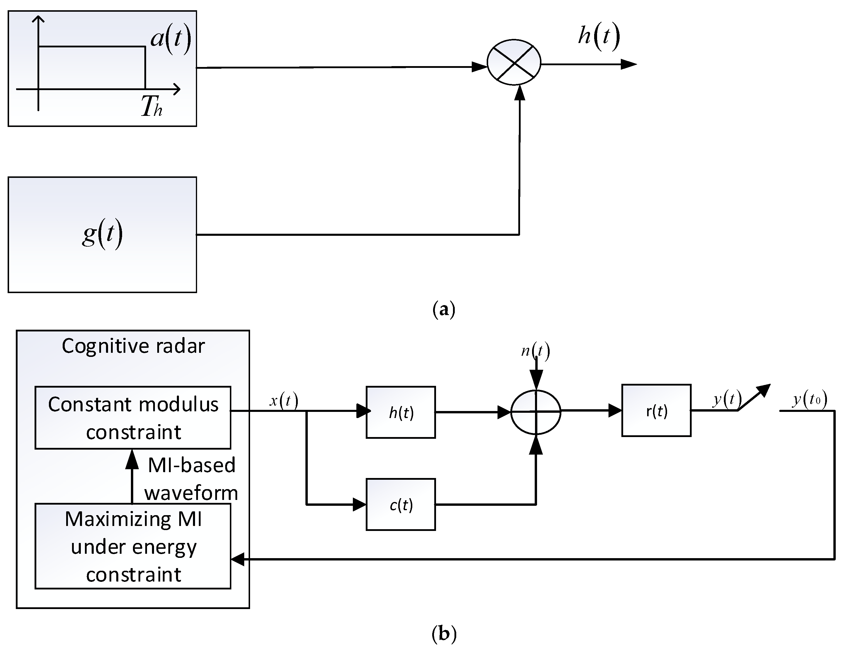
Figure 1a shows the signal model of a random target [10,41], where $a(t)$ is a window function with duration $T_h$, and $g(t)$ denotes a generalized stationary random process. The product $h(t)=a(t)g(t)$ is a finite-duration random process. Figure 1b shows the closed-loop radar echo signal model, where $x(t)$ represents the transmitted signal. $X(f)$ and $H(f)$ represent the Fourier transforms of $x(t)$ and $h(t)$, respectively. $n(t)$ is a zero-mean additive white Gaussian noise with the PSD $Snn(f)$. Likewise, $c(t)$ is signal-dependent clutter with the PSD $Scc(f)$.$r(t)$ denotes the signal model of the receiver filter.

The energy spectrum variance (ESV) of a random target is denoted as (1) [10,41].

$${\sigma }_H^2\left(f\right)={\rm E}\left[{\left|H\left(f\right)-{\mu }_H\left(f\right)\right|}^2\right]$$

(1)

Based on the signal model in Figure 1, the output signal $y(t)$ is

$$y(t)=x(t)\ast h(t)+x(t)\ast c(t)+n(t)$$

(2)

From the knowledge of information theory, maximizing MI is used as the optimization function with the energy constraint. The echo contains more target information by maximizing the MI between the target and echo, which will lead to more accurate estimation and tracking of target parameters. Assume that $E_X$ is the total energy constraint of the transmitted waveform. The optimization model for MI-based waveform ESD can be expressed as (3) [41].

$$\begin{array}{l}\underset{|X\left(f\right){|}^2}{\max }{T}_y{\displaystyle {\int }_B\ln \left[1+\frac{2{\left|X\left(f\right)\right|}^2{\sigma }_H^2(f)}{T_y\{2{\left|X\left(f\right)\right|}^2{S}_{cc}(f)+S_{nn}\left(f\right)\}}\right]df}\\ \mathrm{s}.\mathrm{t}.{\displaystyle {\int }_B{\left|X\left(f\right)\right|}^2}df\le E_X\end{array}$$

(3)

where $B$ represents the bandwidth, and $T_y$ denotes the duration of the echo.

The optimization model (3) could be solved using the Lagrange multiplier method [10]. The MI-based optimal waveform ESD can be expressed as

$${\left|\tilde{X}\left(f\right)\right|}^2=\max \left[0,-R\left(f\right)+\sqrt{R^2\left(f\right)+S\left(f\right)\left(A-D\left(f\right)\right)}\right]$$

(4)

$$D\left(f\right)=\frac{T_y{S}_{nn}\left(f\right)}{2{\sigma }_H^2\left(f\right)}$$

(5)

$$R\left(f\right)=\frac{S_{nn}\left(f\right)\left(2T_y{S}_{cc}\left(f\right)+{\sigma }_H^2\left(f\right)\right)}{4S_{cc}\left(f\right)\left(T_y{S}_{cc}\left(f\right)+{\sigma }_H^2\left(f\right)\right)}$$

(6)

$$S\left(f\right)=\frac{S_{nn}\left(f\right){\sigma }_H^2\left(f\right)}{2S_{cc}\left(f\right)\left(T_y{S}_{cc}\left(f\right)+{\sigma }_H^2\left(f\right)\right)}$$

(7)

A is a constant that is related to the energy.

$${\displaystyle {\int }_B\max \left[0,-R\left(f\right)+\sqrt{R^2\left(f\right)+S\left(f\right)\left(A-D\left(f\right)\right)}\right]}df\le E_X$$

(8)

So far, the MI-based optimal waveform ESD has been obtained, which could match the target characteristics well in the frequency domain. However, it is not concerned with how to synthesize time–domain signals with constant–modulus constraints to satisfy the power amplifiers and other radar transmitter hardware requirements. Constant–modulus constraints make the optimization problem non–convex, which is NP hard to solve. Thus, a new phase–retrieval algorithm based on BFOA is proposed to solve the problem in the next section.

3. The Time–Domain Constant–Modulus Signal Design Base on BFOA

In this section, we first introduce BFOA in order to better understand the proposed phase–retrieval algorithm. Subsequently, the relationship between BFOA and time–domain phase retrieval is presented. Finally, the process of retrieving the optimal phases via the proposed BFOA–based phase–retrieval algorithm is designed.

3.1. Introduction to BFOA

Many engineering problems and scientific research can be modeled as nonlinear optimization problems. Radar waveform optimization is a typical nonlinear optimization problem. BFOA is often employed to tackle nonlinear optimization problems. In addition, radar systems usually have complex design constraints, such as energy consumption, bandwidth, constant modulus, etc. It is difficult to solve the complex optimization model under the multiple constraints by traditional algorithms. Some intelligent optimization algorithms, such as Genetic Algorithm (GA) and Particle Swarm Optimization (PSO), have been applied to solve the kind of complex optimization problems, but BFOA has not attracted attention. BFOA possesses fine local search and global optimization abilities, and BFOA has shown a competitive performance against well–known algorithms such as GA and PSO [42]. In this paper, the synthesis of the optimal time–domain signal under constant modulus and energy constraints is a complex non–convex optimization problem that is NP hard to solve. If the traditional optimization method is used, the whole search space needs to be traversed, and the optimization problems cannot be solved effectively. Based on the characteristics of radar waveform optimization and BFOA, using BFOA to solve the waveform optimization problems is undoubtedly a good choice.

Passino proposed the BFOA in 2002 [34]. Specifically, the foraging behavior of E. coli can be described as follows: E. coli can sense the concentration of nutrients and move to places with high concentrations. The movement modes of E. coli can be divided into swimming and tumbling. Swimming means directional movement, and tumbling means random movement. When the nutrient concentration of the front side is high, E. coli moves by swimming; when the nutrient concentration of the front side is low, E. coli will no longer move forward and will randomly choose a direction to continue swimming by tumbling. The process of BFOA mainly includes the following steps:

(1)

Chemotaxis

Chemotaxis is the fundamental operation of a bacterial foraging optimization algorithm. Bacteria realize local exploration via chemotaxis. Swimming and tumbling are two ways of chemotaxis. The mathematical description of chemotaxis can be expressed as

$${\theta }^i(i,j+1,k,l)={\theta }^i(i,j,k,l)+C(i)\frac{\Delta (i)}{\sqrt{{\Delta }^T(i)\Delta (i)}}$$

(9)

where ${\theta }^i(i,j,k,l)$ represents the position of bacteria $i$ after the $j$-th chemotaxis step, $k$-th is the reproduction step and $l$-th is the elimination and dispersal steps. $C(i)$ is the chemotactic step size. $\Delta (i)$ is the direction phasor.

(2)

Reproduction

After chemotaxis, the bacteria will start to reproduce. The reproduction operation can keep the individuals with high health, and eliminate the individuals with low health, which accelerates the algorithm’s convergence rate. The health of the bacteria can be expressed as

$$J_{health}^i={\displaystyle \sum _{j=1}^{Nc+1}J(i,j,k,l)}$$

(10)

where $N_C$ is the maximum step in a single chemotaxis step, and $J(i,j,k,l)$ represents the nutrient concentrations in the environment when bacteria $i$ is at the current position.

(3)

Elimination and Dispersal

After the reproduction operation, the bacteria may fall into a local optimal position, which obtains a non-global optimal solution. Therefore, the elimination and dispersal operations are introduced to BFOA. The specific process is as follows: Firstly, a fixed elimination probability $P_{ed}$ is initialized. When the elimination probability $P_i$ randomly generated by bacteria $i$ is less than $P_{ed}$, the bacterium will be eliminated, and a new bacterium will be randomly generated within the exploration area. Therefore, elimination and dispersal can partially facilitate the algorithm in escaping the local optima.

3.2. Relationship between BFOA and Time-Domain Phase Retrieval

In order to better apply BFOA to solve time-domain phase-retrieval problems, the relationship between BFOA and time–domain phase retrieval is presented. In time-domain phase–retrieval problems, MMSE is an objective function. Therefore, $MMSE(i)$ is used as the health $J_{health}^i$ to represent the nutrient concentrations in the current position of bacteria $i$. A smaller MMSE represents a higher nutrient concentration at the current position. ${\theta }^i(t,i,j,k,l)$ is used as a substitute for ${\theta }^i(i,j,k,l)$ in order to distinguish the position of bacteria at different sampling times. ${\theta }^i(t,i,j,k,l)$ corresponds to the phases $\phi (t)$ of the time-domain constant-modulus signal in the radar waveform design. The process of bacteria moving toward the highest concentration of nutrients corresponds to the process of retrieving optimal phases. The direction phasor $\Delta (i)$ of the bacteria is fixed, and the bacteria can only move up or down at the current sampling time.

In the process of BFOA, we pay attention to the bacteria’s position ${\theta }^i(t,i,j,k,l)$; ${\theta }^i(t,i,j,k,l)$ corresponds to the phases $\phi (t)$ of the time-domain waveform in the design of a radar waveform. Via chemotaxis, reproduction, elimination, and dispersal, the bacteria move to places where the nutrient concentration is higher (the MMSE is smaller) and stop moving when the global optimum phase is retrieved. Finally, the optimal phase is retrieved at each sampling time.

3.3. The Phase–Retrieval Algorithm Based on BFOA

Assuming that the transmitted signal is a nonlinear frequency modulation signal, $\phi (t)$ is a time–domain dependent phase function, and $c$ is the constant amplitude of the signal. The transmitted signal is expressed as

$$x(t)=c{e}^{j\phi (t)},t\in [-T/2,T/2]$$

(11)

Obtaining $x(n)$ after discrete sampling in the time domain can be expressed as follows:

$$x(n)=c[e^{j{\phi }_0},e^{j{\phi }_1},e^{j{\phi }_2},\dots ,e^{j{\phi }_{N-1}}]$$

(12)

where $n=0,1,2,3,\dots ,N-1$, $\phi ={[{\phi }_0,{\phi }_1,\dots ,{\phi }_{N-1}]}^T$. The N–point Discrete Fourier Transform (DFT) of $x(n)$ is

$$X(k)={\displaystyle \sum _{n=0}^{N-1}x(n)e^{-j2\pi kn/N}}$$

(13)

where $k=0,1,2,3,\dots ,N-1$.

Let ${\left|X(k)\right|}^2$ be the constant-modulus signal ESD. In Section 2, the optimal waveform ESD ${\left|X\left(f\right)\right|}^2$ is obtained under energy constraints. Let ${\epsilon }_{opt}(k)$ be the discrete sampling of ${\left|X\left(f\right)\right|}^2$. MMSE in the frequency domain between ${\left|X(k)\right|}^2$ and ${\epsilon }_{opt}(k)$ is used as the cost function to represent the nutrient concentrations of the current position. Thus, the MMSE can be expressed as (14).

$$\mathrm{E}(\phi )=\frac{1}{N}{\displaystyle \sum _{k=0}^{N-1}{({\epsilon }_{opt}(k)-{\left|X(k)\right|}^2)}^2}$$

(14)

When the MMSE is smaller, the error between the BFOA-based constant-modulus signal ESD and the MI–based waveform ESD is smaller, which indicates that the time-domain signal has a slight performance degradation. On the contrary, it means a large performance loss. In order to minimize $E(\phi )$, the BFOA–based phase–retrieval algorithm is presented to search optimal time–domain phases $\widehat{\phi }$. BFOA is the core of the proposed phase–retrieval algorithm. A certain number of bacteria are distributed from 0 to $2\pi$ at each sampling time. Each bacterium moves up and down at the current sampling time (search space) to find the optimal phase (optimal position) until it finds the optimal phase. Via chemotaxis, reproduction, elimination, and dispersal operations, bacteria constantly lean toward the optimal location and avoid blindly searching the entire search space. The BFOA–based phase–retrieval algorithm monotonically reduces the spectral mean square error at each iteration. The BFOA–based phase–retrieval algorithm is summarized in

Table 3. The proposed phase–retrieval algorithm based on BFOA.

1:	$p\leftarrow 0$
2:	${\widehat{\phi }}^p\leftarrow$ random initialization over $\left[0,2\pi \right)$
3:	repeat
4:	${\widehat{\phi }}^p\leftarrow$BFOA (chemotaxis, reproduction, elimination, and dispersal)
5:	${\widehat{\phi }}^{p+1}\leftarrow {{\phi }^{\prime }}^p$, if $E({{\phi }^{\prime }}^p)<E({\widehat{\phi }}^p)$
6:	${\widehat{\phi }}^{p+1}\leftarrow {\widehat{\phi }}^p$, else
7:	$p\leftarrow p+1$
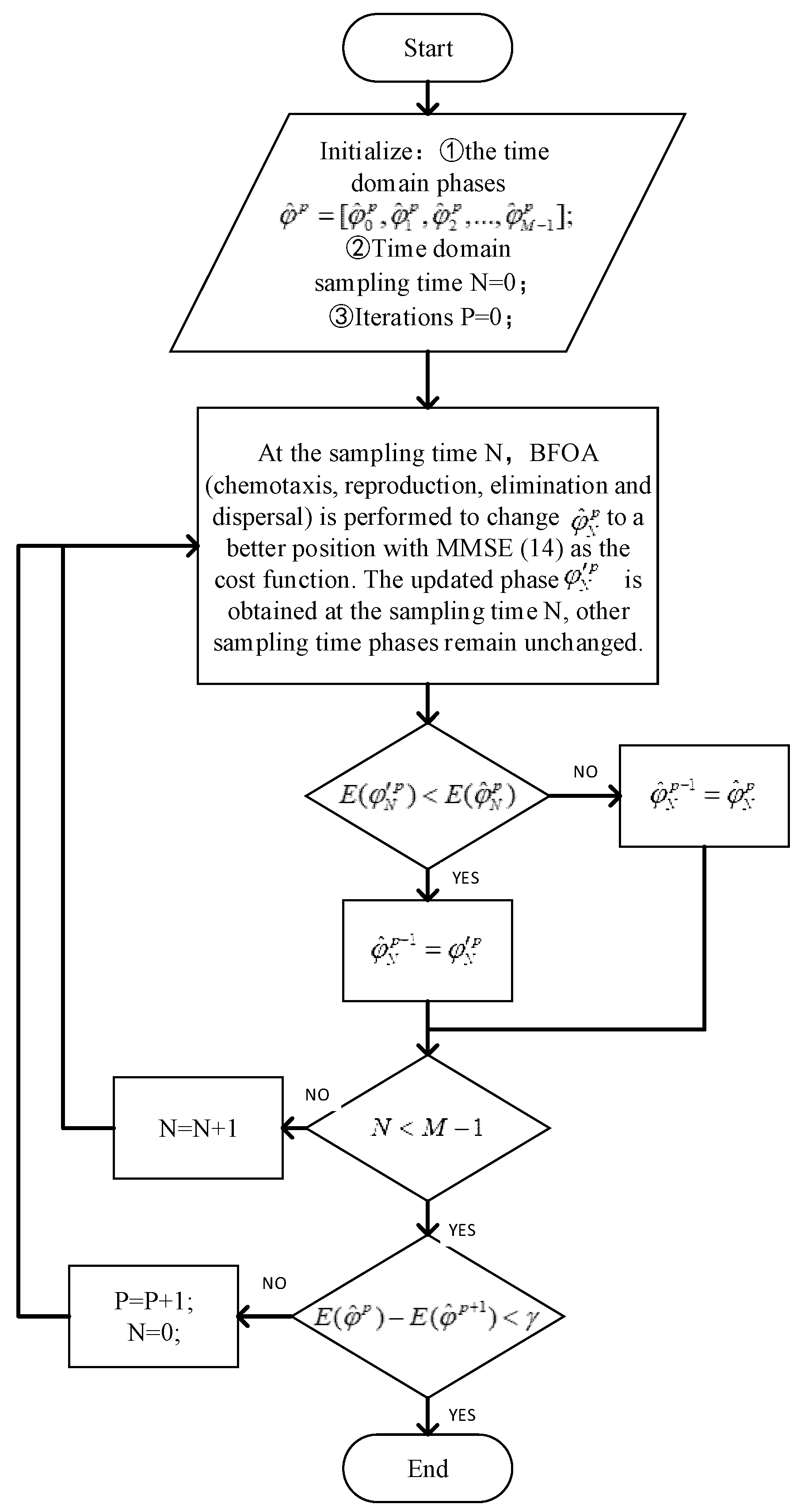
8:	until $E({\widehat{\phi }}^{p-1})-E({\widehat{\phi }}^p)<\gamma$, where $\gamma$ is a predefined threshold.

. The flowchart of the proposed phase–retrieval algorithm based on BFOA is shown in Figure 2.

Initially, the phase $\widehat{\phi }$ of the discrete-time-domain signal is randomly initialized, and the MMSE (14) is calculated. Subsequently, at each sampling time, bacteria undergo chemotaxis, reproduction, elimination, and dispersal operations sequentially to obtain updated phase ${\phi }^{\prime }$ and MMSE (14). If the updated MMSE (14) decreases, $\widehat{\phi }={\phi }^{\prime }$, otherwise, the phase $\widehat{\phi }$ remains unchanged. This process continues until the change in MMSE (14) between two iterations falls below a predefined threshold value $\gamma$, ending the loop.

The complexity of the BFOA-based algorithm depends on the model of the optimization problem. In this paper, MMSE (14) is calculated and compared every time the bacteria move to a new location with computational complexity of $O(N\log N)$, and the number of bacterial movements during each iteration increases linearly to factors such as the number of bacteria $S$, the number of sampling points $N$, the number of chemotaxis $N_c$, the number of reproduction $N_{re}$, and the number of eliminations and dispersal $N_{ed}$. Consequently, the proposed algorithm exhibits a complexity of $O(S{N}_c{N}_{re}{N}_{ed}{N}^2\log N)$.

4. Simulations and Discussion

In the simulation design process, simulation parameters are shown in

Table 4. Simulation parameters.

Symbol	Description	Value
$S_{nn}(f)$	the noise PSD	0.1
$T_y$	the echo duration time	2 μs
$N$	the sampling points	128
$E_x$	transmitted waveform energy	0.4
$c$	modulus	0.056
$S$	the number of bacteria at each sampling point	10
$\phi$	the initial phases	$[0,2\pi )$
$N_c$	bacterial chemotaxis times	30
$C$	chemotactic step size of bacteria	0.04
$N_s$	the maximum swimming times	4
$N_{re}$	bacterial reproduction times	4
$N_{ed}$	bacterial elimination and dispersal times	2
$P_{ed}$	elimination probability	0.25
$\gamma$	threshold	0.01
$p$	the maximum iterations	50
$\Delta (i)$	the direction phasor	90°

. The qualitative performance of the simulation results is not significantly affected by the simulation parameters of energy $E_x$, echo duration time $T_y$, and modulus $c$. Our primary concern lies in the energy distribution mode of the waveform rather than its numerical size. The initial phases of the time-domain signals are randomly assigned within a range of $[0,2\pi )$, it should be noted that any phase value can be chosen without significant impact on the results. The maximum iterations $p=50$ and the threshold value $\gamma =0.01$ are determined based on empirical simulations. The termination condition for the loop is set as the MMSE change between consecutive iterations being smaller than a threshold value $\gamma$. This choice of $\gamma =0.01$ indicates that the improvement in MMSE has reached a sufficiently small level, and the threshold value can be further reduced theoretically. The direction phasor $\Delta (i)={90}^{\mathrm{o}}$ which restricts bacterial movement solely in the vertical direction during the current sampling time.

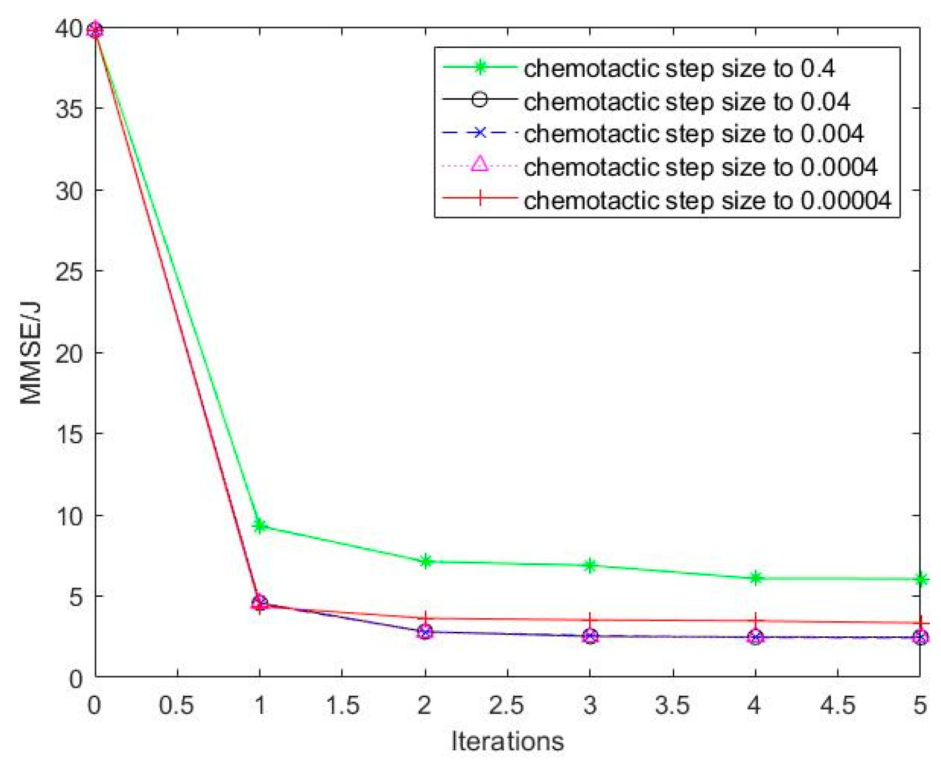
The BFOA involves various parameters, and many parameters have a great influence on the performance and efficiency of the algorithm, including the number of bacteria, chemotactic step size, chemotaxis times, reproduction times, elimination and dispersal times, etc. Although increasing the number of bacteria and the chemotaxis times can improve the optimization ability of the algorithm, it also increases the calculation amount of computation. Choosing the optimal parameters to achieve optimal performance is a complex optimization problem. We carried out a lot of simulations of the parameters based on experience. Taking the chemotactic step size as an example, as shown in Figure 3, the X-axis represents iterations, and the Y-axis uses MMSE to evaluate the performance of the algorithm. The smaller the MMSE, the better the algorithm’s performance. We set the chemotactic step sizes to 0.4, 0.04, 0.004, 0.0004, and 0.00004. It can be seen in Figure 3 that the algorithm performs worst when the chemotactic step size is 0.4; with the decrease in the chemotactic step size, bacteria perform more precise searches, and the algorithm performs better, but as the chemotactic step size decreases further to 0.00004, bacteria search only in a limited area, the global optima cannot be searched, and the algorithm performs worse. The algorithm’s performance has little difference when the chemotactic step size is 0.04, 0.004, and 0.0004. We chose a larger chemotactic step size so that the global optima could be searched with fewer chemotactic times. Therefore, we set the chemotactic step size to 0.04.

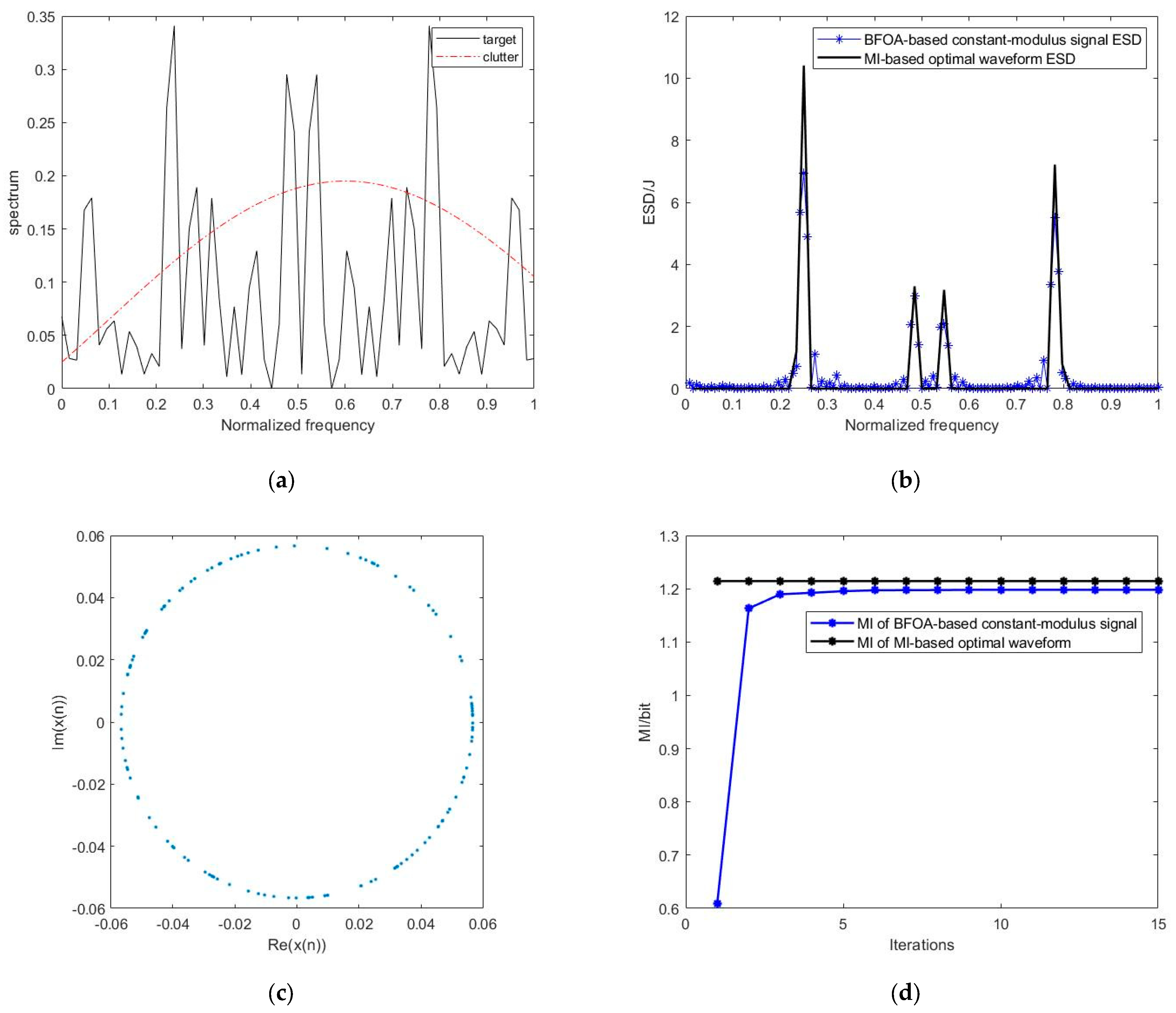
In the simulation design process, white Gaussian noise is used; it reflects the additive noise in the real channel to some extent, and it can be expressed via specific mathematical expressions, which is convenient for derivation, analysis, and calculation. The following scenario is considered. The additive white Gaussian noise PSD $S_{nn}(f)=0.1$. The spectra of target and clutter are shown in Figure 4a.

The BFOA–based constant–modulus signal ESD under energy and constant–modulus constraints and MI–based optimal waveform ESD under energy constraints are illustrated in Figure 4b. It shows that the time–domain constant–modulus signal ESD is similar to the MI–based optimal waveform ESD. For BFOA–based constant–modulus signal ESD, the four peak amplitudes are also maintained, which could match the target characteristics well in the frequency domain. And less energy is spread into additional frequency bands.

Figure 4c illustrates a synthesized time–domain signal by using the BFOA-based phase–retrieval algorithm has a constant amplitude, which can maximize the utilization of the transmitter power and meet the hardware requirements of radar transmitters.

Figure 4d shows the MI performance of the BFOA–based constant–modulus signal. The MI corresponding to the BFOA–based constant–modulus signal becomes monotonically closer to that corresponding to the MI–based optimal waveform. It shows that the proposed BFOA–based time–domain signal synthesis algorithm possesses several advantages, including monotonically increasing MI, a small MI loss, and converging with a few iterations.

The above simulation verifies that the proposed BFOA-based phase-retrieval algorithm can synthesize a time–domain constant–modulus signal. The synthesized signal ESD retains the characteristics of MI–based optimal waveform ESD. There is only a small performance loss for radar–transmitted signals after adding constant-modulus constraints. In non-convex optimization problems, initial values have a great influence on the performance and final results of traditional algorithms. To further validate the proposed algorithm’s sensitivity to initial phases during the iterative process, we consider the following scenario. The initial phase is changed, and the other parameters remain the same; simulation results are shown in Figure 5.

As shown in Figure 5a, the synthesized constant–modulus signal’s ESDs with different random initial phases are approximate. Random initial phases will not affect the algorithm’s synthesis of the time–domain constant–modulus signal. As shown in Figure 5b, MMSEs of different random initial phases decrease monotonically with the increase in iterations, and eventually, they all converge to a similar solution. Therefore, the proposed phase–retrieval algorithm based on BFOA is insensitivity to initial phases.

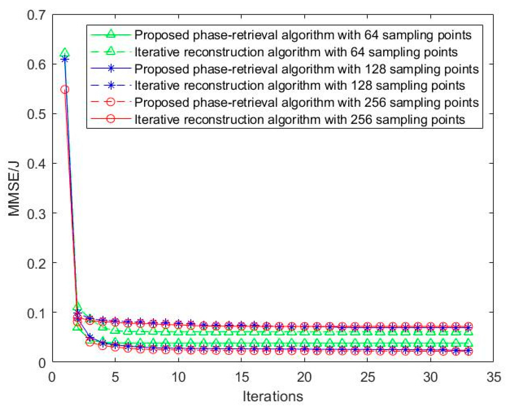
To further validate the proposed algorithm’s sensitivity to sampling points during the iterative process, the following scenario is considered. The number of sampling points is 64, 128, and 256, respectively, and the other parameters remain the same; simulation results are shown in Figure 6.

As illustrated in Figure 6a, synthesized constant–modulus signals’ ESDs with different sampling points all retain the characteristics of the MI–based optimal waveform ESD. As shown in Figure 6b, the MMSEs corresponding to the different number of sampling points decrease monotonically with the increases in iterations. Eventually, they all converge to a similar solution, and MMSE will decrease slightly with the increase in sampling points. The performance of the BFOA–based phase–retrieval algorithm will improve with the increase in sampling points.

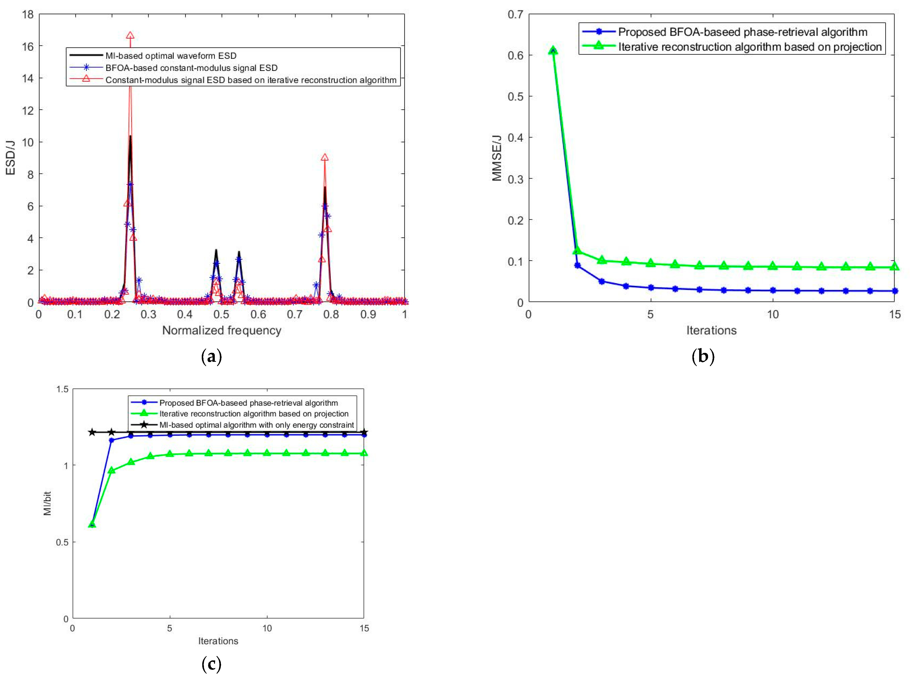
We also compare the proposed BFOA-based phase-retrieval algorithm with the iterative reconstruction algorithm based on projection [17]. Both algorithms use the same parameters and set the number of sampling points to 128. Figure 7a shows the constant–modulus signal’s ESD synthesized using the proposed phase–retrieval algorithm and the iterative reconstruction algorithm, which are shown by blue and red lines, respectively. The two time–domain waveform synthesis algorithms both retain the spectral characteristics of the MI–based optimal waveform ESD. But, the synthesized signal’s ESD by the proposed algorithm matches the MI–based optimal waveform ESD better.

Figure 7b,c show the MMSEs and MIs corresponding to the two algorithms, respectively. The synthesized time–domain constant–modulus signal based on BFOA has a smaller MMSE and more MI than the synthesized time-domain signal based on an iterative reconstruction algorithm. It shows that the proposed algorithm achieves better performance compared with the iterative reconstruction algorithm. A better time–domain constant–modulus signal will be obtained using the proposed time–domain signal synthesis algorithm.

It is worth noting that the proposed algorithm has a higher complexity than the iterative reconstruction algorithm. The algorithm’s complexity increases with the increase in sampling points, the number of bacteria, chemotaxis times, reproduction times, and elimination times.

To further compare the two algorithms, we compare the two algorithms with different sampling points. Both algorithms fast converge, and MMSEs decrease monotonically with the increase in iterations. Moreover, as shown in Figure 8, no matter how the sampling number changes, the proposed algorithm based on BFOA obtains a smaller MMSE than the iterative reconstruction algorithm.

5. Conclusions

In this paper, we first review the method of MI–based optimal waveform ESD, and then consider the time–domain transmitted signal should have a constant modulus to meet the actual requirement of the radar transmitters. A new BFOA–based phase–retrieval algorithm is proposed to synthesize a time–domain constant–modulus signal with the characteristics of MI–based optimal waveform ESD. The proposed phase–retrieval algorithm searches for the optimal phases at each sampling point with the MMSE in the frequency domain as the cost function. It can be used to solve multi–constraint optimization problems. Simulation results demonstrate the satisfied constant–modulus signal can be synthesized by the proposed algorithm with only a few iterations, and the proposed algorithm has a smaller MI loss and MMSE compared with the iterative reconstruction algorithm based on projection [17]. In addition, the proposed algorithm is insensitive to initial phases and performs better with the increase in sampling points.

Future work might include further employing BFOA to address complex non–convex optimization problems in the field of radar waveform optimization. Considering the existence of jammers, noise, and interference signals are strong, to ensure effective radar target detection, incorporating SINR constraint as one of the constraints is imperative. As the complexity of the optimization model increases, BFOA outperforms traditional algorithms. The adaptive chemotactic step size and migration operator will be further designed according to the current iteration number and position, aiming to enhance the algorithm’s search capability and reduce its complexity.