Abstract
Autonomous robotic swarms are envisioned for a variety of applications—for example, space exploration, search and rescue, and disaster management. Important features of a robotic swarm include its ability to share information within the network, to sense spatio-temporal processes such as gas distributions, and to collaboratively enhance its navigation. In environments without infrastructure, the swarm elements can cooperatively estimate their position, e.g., based on the time of flight of exchanged radio signals. Cooperative positioning performance depends on the radio propagation environment. Free-space path loss is commonly used for performance assessment, which is an optimistic assumption. In this work, we investigate the limits to cooperative positioning and ranging based on the time of flight of radio signals over the more realistic two-ray ground reflection channel. We show that we obtain a ranging bias caused by the radio signal component reflected from the ground, and that the ranging error becomes bias-limited. In the positioning domain, we investigate how the ranging bias affects the cooperative positioning performance. As a result, we gain in cooperation, but the achievable positioning performance is significantly worsened by the ranging bias. As a conclusion, the two-ray ground reflection model should be considered to obtain realistic cooperative positioning limits.
1. Introduction
Autonomous robotic swarms are envisioned for a large variety of applications on Earth and in space. On Earth, they can be used for search and rescue missions, disaster management after natural or industrial disasters, and environmental monitoring [1,2]. In space, we envision robotic swarms and scientific instruments deployed on the lunar or Martian surface for exploration; see Figure 1 [3,4,5,6]. An important feature of a robotic swarm is its ability to share information about its sensed environment, its current state, and the robustness to failure of swarm elements [7,8]. For example, a robotic swarm can sense spatio-temporal processes such as gas distributions in a distributed fashion [9]. Every exploration of a physical phenomenon requires position information, timing information, and communication. Infrastructure is commonly not available for, e.g., lunar exploration; see Figure 1. GNSS (global navigation satellite system)-based positioning, and satellite or cellular communications are not available. However, we can see the robotic swarm and all sensors deployed as instrument packages in Figure 1 as one cooperative network [10]. Wireless communication is established by exchanging radio signals. These radio signals can then be used for ranging: a distance estimate among all entities is obtained by estimating the ToF (time of flight) or RTT (round trip time) of the radio signal [11,12]. Ranging estimates are subsequently used to estimate the position of each swarm-element. We distinguish two positioning techniques, namely non-cooperative and cooperative positioning [12,13]. In non-cooperative positioning, ranging estimates between a swarm-element and so called anchors are used. Anchors are entities with known position, for example, the lander and two instrument packages closely deployed to the lander; see Figure 1. In practice, not all swarm-elements have connectivity to the anchors due to path loss or shadowing caused by the terrain. Cooperation is the solution, where swarm-elements obtain ranging estimates. The position of each swarm-element can then be estimated cooperatively in a centralized or decentralized fashion [13,14].
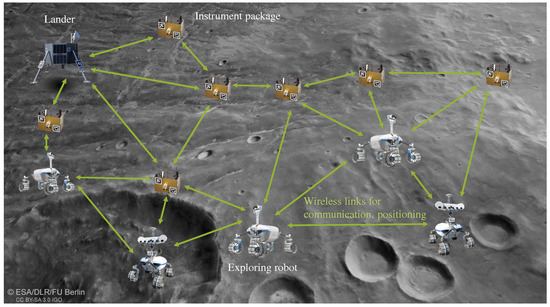
Figure 1.
Lunar robotic swarm exploration scenario with multiple robots and instrument packages deployed on the lunar surface. All entities are connected with wireless links enabling communication, ranging and positioning. Infrastructure for communication and radio navigation is not available.
The design of a a wireless system jointly enabling communications, ranging and positioning, is based on models for radio-propagation, methods to predict the achievable positioning performance, and algorithms for estimation [15]. Commonly, the ranging variance and positioning error are predicted based on the CRBs (Cramér-Rao bounds) [16,17]. The CRB enables us to assess the precision of an unbiased estimator given a particular system model [18]. For positioning, a common assumption is free-space path loss propagation of the LoS (line-of-sight) signal between a transmitter and a receiver for an environment, as shown in Figure 1. However, this assumption is too optimistic. Based on empirical results from a space-analog experiment on the volcano Mt. Etna, Italy, in 2022 [19,20], we found that our ranging estimates partly contain a negative bias. We set up the hypothesis that this effect could be caused by the radio signal component reflected from the ground, which is the motivation for this work.
In this work, we investigate limits on cooperative positioning for a robotic swarm exploring the lunar surface. We especially focus on the two-ray ground reflection channel. We investigate in detail the ranging variance and the ranging bias for this radio channel model. From ranging domain, we move to the positioning domain and show how the positioning performance degrades with the obtained ranging variance and ranging bias. In addition, we show how the average positioning error improves with an increasing number of swarm-elements in cooperative positioning, even though the ranging error is dominated by the ranging bias. We use the free-space path loss model as reference for comparison to existing works.
This paper is organized as follows: in Section 2, we introduce the two-ray ground reflection channel model, the system model for ranging, the ML (maximum likelihood) estimator and the CRB for ranging. The resulting ranging performance is presented in Section 3. We move from ranging domain to positioning domain in Section 4, looking at single-swarm element positioning and cooperative positioning. Lower bounds, and the ML positioning estimator are presented. In Section 5, we present the non-cooperative positioning performance of a single swarm-element. Cooperative positioning performance results are shown in Section 6. We conclude in Section 7 and provide an outlook of future research directions in Section 8.
2. Time of Flight Ranging
In this section, we recapitulate the two-ray ground reflection channel model, and introduce the system model for ToF-based ranging. To evaluate ranging performance in Section 3, we introduce the ML estimator, followed by the CRB for distance estimation.
2.1. Two-Ray Ground Reflection Channel
The two-ray ground reflection channel is commonly used to model large-scale fading in various wireless communication applications [21,22]. Figure 2 shows the geometry. Transmitter and receiver are at height and , respectively, and separated by the horizontal distance . The first ray is the LoS component with its distance denoted as d, with if . The second ray is the component reflected from the ground with its equivalent distance . Based on this geometry, the two signal components observed by the receiver are
and
with transmitted signal , carrier wavelength , and reflection coefficient . We assume unity antenna gain for all angles for both, transmitter and receiver, and specular ground reflection only. The carrier wavelength is defined as , with as speed of light in vacuum, and carrier frequency . The reflection coefficient is defined as
with an assumed vertical polarization, such that
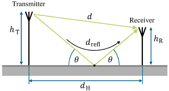
Figure 2.
Geometry for two-ray ground reflection channel model.
The incident angle of the reflected signal component is captured in , and the electrical properties of the ground in . We assume specular reflection only, and discard diffraction loss caused by surface roughness. The permittivity of the ground consists of two components: the relative permittivity as the real part and the conductivity as the imaginary part. In general, conductivity is found as so-called tangent loss in the literature and the imaginary part of can be set as tangent loss multiplied by the relative permittivity. In this work, we consider a real-valued only, as we assume a very low-conductive soil. Additionally, we consider to be constant for the carrier frequency range under investigation.
Both received signal components are subject to FSPL (free-space path loss) and superpose constructively or destructively depending on the carrier phase. Hence, we will observe a distance dependency of the received signal power. By considering a narrow-band transmitted signal , we can determine the total received signal power
with the carrier phase difference defined as
2.2. System Model
In the following, we describe a generalized system model for ToF-based ranging between a transmitter and receiver. We assume OFDM (orthogonal frequency-division multiplexing) modulation as a state-of-the-art modulation technique. Our qualitative results are valid for other waveforms and our presented approach can be applied accordingly.
Our transmission model depicted in Figure 3 comprises a multi-carrier transmitter and multi-carrier receiver based on OFDM. We assume that the transmitter and receiver are perfectly time-synchronized to enable ToF-based ranging. In practice, one would choose a multi-way ranging technique such as TWR (two-way ranging). We define a sampling interval as the inverse of the sampling frequency and describe the sampled and transmitted OFDM symbol in time-domain as
with n as sample index in the range , and k as subcarrier index. The OFDM symbol consists of N even subcarriers with a C samples long cyclic prefix. In a practical implementation, we need to keep guard bands at the spectrum’s edge for low-pass filtering. Consequently, only usable subcarriers can be allocated, yet the power of the transmitted signal is normalized to one. We obtain the received signal with additive Gaussian distributed white noise with zero mean and variance represented by as
which is the convolution of the transmitted OFDM signal with the CIR (channel impulse response) . With (1) and (2), we can express the CIR as sum of weighted Dirac delta functions
with as complex amplitude of the LoS component with and the reflected component . We define propagation delays as with and . (10) reduces to a single-path CIR with in the free-space path loss case without the ground reflection component.
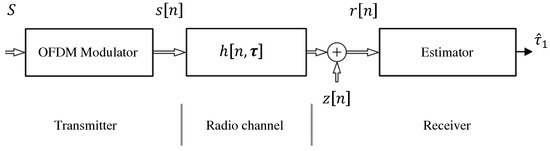
Figure 3.
Transmission model for OFDM based ToF ranging.
2.3. Maximum-Likelihood Estimator
We are interested in estimating , for which we need to estimate . The estimator depicted in Figure 3, consisting of an ML estimator assuming a single-path radio channel. As shown in [23], this ML estimator can be realized as single-tap correlation receiver, equivalent to a DLL (delay-locked loop) in GNSS receivers. We focus on snapshot-based estimation, where only one received OFDM symbol is used for estimation and no tracking is applied. The ML estimator to incoherently estimate the delay of the LoS component therefore corresponds to
assuming unknown phase offset between transmitter and receiver. The correlation length is equivalent to the OFDM symbol length N. By using OFDM, we can shift the correlation from the time domain into the frequency domain to avoid costly signal interpolations in the time domain for sub-sample delay estimation. The incoherent delay estimation in the frequency domain is
Ranging is commonly divided into two steps: an acquisition step and a fine synchronization step. In the acquisition step, the correlation function in (12) is evaluated on a time grid, which contains integer multiples of the receiver’s sampling interval . This can be efficiently realized via FFT (fast Fourier transform) and IFFT (inverse fast Fourier transform). The maximum of this coarse grid correlation function is detected and its correlation lag is used as initialization for fine synchronization. We can see from (12) that we optimize with respect to the strongest path only, assuming that the LoS component used for ranging is the strongest path. The radio channel itself as defined in (10) comprises two components. As a result, our ML estimator will be biased.
2.4. Lower Bound on Ranging Variance
In addition to the ranging estimate from (12), we are interested on lower bounding the ranging variance. We recall a commonly known lower bound for the ranging variance, as we are interested in the resulting ranging precision based on the received signal power and, hence, the SNR (signal to noise ratio) of the received signal.
One common method to quantify the precision of an unbiased estimator is the CRB. In general, we can find the CRB for ToF-based ranging as follows
where represents the SNR, and the so-called effective or equivalent bandwidth
A larger SNR and a larger equivalent bandwidth result in a lower ranging variance. For ToF-based ranging with OFDM signals, the CRB for the distance estimate states
with noise variance , OFDM subcarrier spacing , and the signal power allocated at subcarrier index k.
3. Ranging Performance Results
In the following sections, we take a detailed look at the resulting ranging performance. We define ranging precision as the variance, ranging accuracy as the bias, and ranging performance as the RMSE (root mean square error), respectively. Unless otherwise stated, we use system parameters from Table 1. We assume a low-power WiFi such as OFDM transmission system with a signal bandwidth of 20 and 1 transmit power. At the receiver, we do not include an additional noise figure to the thermal noise, to keep results comparable. Furthermore, we assume a flat terrain.

Table 1.
System parameters.
We assume a relative ground permittivity of as a representative value for lunar regolith and Titanium-Ilmenite [24,25,26]. Relative permittivity values between 2 and 6 are reported and are in a similar value range as volcanic ash and basalt rocks [25,26,27]. The tangent loss is very small; hence, we neglect the imaginary part of the relative ground permittivity [24]. For comparison, an also relates to a very dry sandy soil [28]. We also investigated how a larger influences our results. This investigation is beyond the scope of this paper, but we can say that unless the is greatly increased, e.g., such as for very wet soil or seawater, the results are very similar.
3.1. Ranging Variance
Let us have a look at the first results, and for a more intuitive assessment, we depict the ranging standard deviation . Figure 4 shows the ranging standard deviation over a horizontal distance from 1 to 10 for a transmitter and receiver height of m. This low antenna height is representative of micro-rovers or instrument packages. We apply (15) with system parameters from Table 1. The noise variance is determined based on the receiver SNR for the free-space path loss and the two-ray ground reflection case, respectively. We clearly see the linear increase in in the log–log domain for the free-space path loss case. The radio signal component reflected from the ground results in a -dependent received signal power variation, and thus, a variation of SNR and . The red curve in Figure 4 shows this clearly. At a of about 150 , we observe that the steepness of is a factor of two in the log–log domain compared to one for the free-space path loss case. This transition point is commonly called the breakpoint distance.
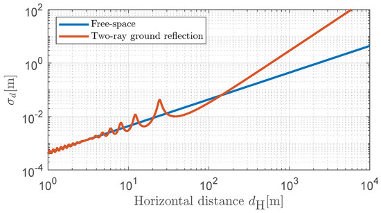
Figure 4.
Ranging standard deviation over horizontal distance . Transmitter height and receiver height .
The received signal power—see (6)—is also dependent on the transmitter and receiver height. Figure 5 shows the results if the transmitter height is increased from to . The breakpoint distance increases from about 150 to about 820 . Furthermore, we experience more fades and more variations in .
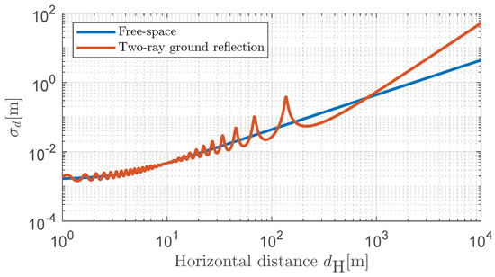
Figure 5.
Ranging standard deviation over horizontal distance . Transmitter height and receiver height .
3.2. Ranging Bias
Besides the ranging variance, determined by the SNR, we are also interested in the ranging bias, denoted as . The radio channel defined in (10) consists of two signal components, yet the estimator in (12) assumes a single signal component only. Propagation delay differences between the LoS component and the ground-reflected component become very small with increasing , and thus are only a very small fraction of the sample length. The used signal bandwidth from Table 1 relates to a sample length of . We therefore expect that a -dependent ranging bias as the second signal component cannot be resolved by the estimator, and have a closer look at some results. The investigation of the ranging bias in this work is closely related to, e.g., the MEE (multipath error envelope) determination in GNSS signal design. The main difference is that the relative signal component amplitudes, phases, and delays are determined by (1) and (2). We determine the ranging bias by applying (12) without additive white Gaussian distributed noise.
Figure 6 shows the resulting ranging bias for three selected carrier frequencies with transmitter and receiver at a height of , and we observe multiple effects. Firstly, an absolute ranging bias up to 20 , with a dominating negative , clear -dependency, and convergence to 0 for large . Secondly, a higher carrier frequency results in more rapid variations along , and peaks at the fading of the received signal power. Thirdly, we see an envelope bounding the ranging bias variations, with a minimum at around 3 . This envelope is driven by the geometry, whereas the variations are driven by the carrier frequency. At we reach the Brewster angle, at which the signal component towards the ground is absorbed. The Brewster angle is a function of the relative permittivity only.
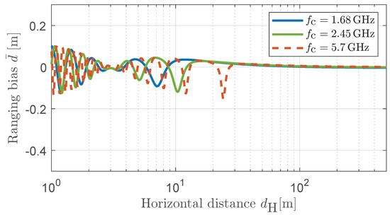
Figure 6.
Ranging bias over horizontal distance for three selected carrier frequencies . Transmitter height and receiver height .
Figure 7 shows the ranging bias if we increase the transmitter height to , representative for, e.g., a lander. The same effects as in Figure 6 can be observed, with two major differences. First, the Brewster angle is at a of about 10 compared to 3 in the previous case, due to the changed geometry. The second difference is the significantly increased absolute value of the ranging bias.
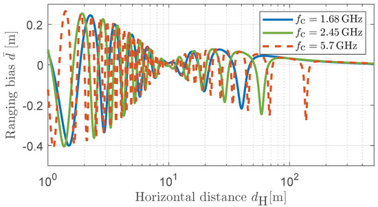
Figure 7.
Ranging bias over horizontal distance for three selected carrier frequencies . Transmitter height and receiver height .
To obtain a better understanding of the influence of the carrier frequency on the ranging bias variations, we determine for carrier frequencies from 1 to 7 . Figure 8 shows the result for a transmitter and receiver antenna height of m each. We will use these height values in the remainder of the paper to represent a setup such as a robot with an antenna pole. Our results provide insight how, e.g., the ranging bias will change at a specific horizontal distance if one selects a different carrier frequency for ranging.
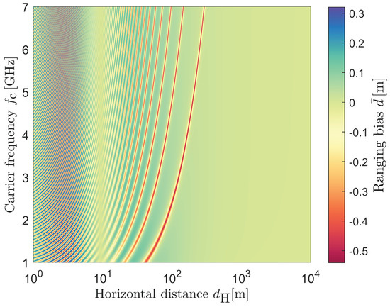
Figure 8.
Ranging bias over horizontal distance for carrier frequencies between 1 and 7 . Transmitter height and receiver height .
3.3. Ranging RMSE
In the previous two sections, we investigated the ranging variance and ranging bias independently and noticed that the ranging bias is generally larger than the ranging standard deviation. As a final result for this ranging section, we calculate the ranging RMSE over based on the bound on the conditional MSE (mean square error) [29]. Figure 9 shows the ranging variance and the ranging RMSE for the system parameters in Table 1 with a transmitter and receiver height of each.
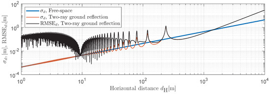
Figure 9.
Ranging RMSE and standard deviation over horizontal distance . Transmitter height and receiver height .
We can see that up to a distance of 100 , we obtain a significantly larger ranging error compared to the unbiased case. At close distances, the RMSE is 1–2 magnitudes larger compared to the predicted ranging standard deviation. We can obtain three important findings from this final result. Firstly, the ranging variance obtained from the CRB, even with the two-ray ground reflection model, is insufficient to model the ranging error adequately. Secondly, a practical ranging system will be bias-limited and not noise-limited. Thirdly, for this given geometry, increasing the transmit power, as well as increasing the signal bandwidth does not improve the ranging error. Increasing the transmit power will result in a lower ranging variance; however, as we are bias-limited, we will not see an RMSE improvement—see, for example, Figure 9 for horizontal distances below 200 . The delay difference between the LoS component and the ground-reflected component is very small, and thus only a very small fraction of the signal sample length. Even for a signal bandwidth of, e.g., 200 , we obtain a negligible improvement only with respect to the ranging bias. A statement regarding an even increased signal bandwidth cannot be made in this work due to our narrow-band signal assumption and applied signal model. However, as the ranging bias is heavily geometry-dependent, a slightly increased signal bandwidth can lower the ranging bias for a different geometry. As a consequence, the ranging RMSE comprising the ranging standard deviation and ranging bias should always be evaluated for new geometries.
4. Cooperative Positioning
In this section, we move from the ranging domain to positioning domain, and look at the lower bounds and the ML estimator. We investigate 2D (two-dimensional) positioning, and the extension to 3D (three-dimensional) is straightforward. Let us start with the scenario depicted in Figure 10, where we have a set of L anchors at known positions . The swarm elements are located at unknown positions . Our goal is to estimate the position of each swarm element based on observations of the distances between anchors and swarm elements, as well as among swarm elements. A key element of cooperative positioning are the ranging links among swarm elements.
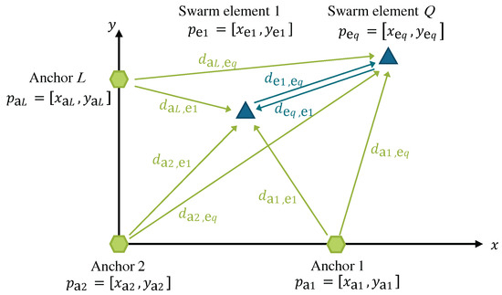
Figure 10.
Positioning of two swarm elements based on distance observations. Anchors have known position, and ranging links among swarm elements are used for cooperative positioning.
4.1. Lower Bound on Positioning Variance
Let us recapitulate the CRB for single swarm-element positioning, as well as cooperative positioning. We define the observed distances between anchors and swarm elements with
and among swarm elements with
The true distances and are corrupted by real valued additive white Gaussian noise and , respectively. The noise variables have zero mean and variances and . Based on (15), we can determine the value for the ranging variance.
4.1.1. Non-Cooperative Positioning
We start with single swarm-element positioning and expand to multi swarm-element positioning without cooperation. This provides the basis to extend the cooperative case in the next subsection.
We wish to estimate the coordinates of swarm element 1, , with unknown parameters and L distance observations. The CRB is defined as the inverse of the FIM (Fisher information matrix)
with for our single swarm-element, 2D positioning case. We can express the FIM with the Jacobian matrix as
The Jacobian matrix contains the partial derivatives of with respect to our K unknown parameters, defined as
and has the size . In our example, for 2D positioning with and , we can determine the Jacobian matrix
where the partial derivatives are the components of the gradient
We now extend the positioning problem to two swarm elements. In the absence of distance observations among swarm elements, we can define the Jacobian matrix for our 2D scenario as
The resulting Jacobian matrix has a block diagonal structure, and additional swarm elements can be added by extending the diagonal structure. Due to the block diagonal structure of the Jacobian matrix, the FIM is block diagonal as well, where each block is related to one swarm element. As a result, the CRB can be calculated by inverting the diagonal blocks of the FIM separately. This also means that we have no coupling for the estimation of each swarm element’s state. The ranging variances required to calculate the FIM, as in (19) are defined as
4.1.2. Cooperative Positioning
For cooperative positioning, we additionally include distance observations among swarm elements—see (17)—and keep our scenario with the two swarm-elements. We can extend the Jacobian matrix (23) with the gradients of the inter-swarm-element distance observations
These gradients add additional rows to (23) and the Jacobian matrix becomes
To calculate the FIM from (19), we also need to provide ranging variances and we extend (24) with the ranging variances of the link between the two swarm elements to
Equations (25)–(27) can be generalized for an arbitrary number of swarm elements.
4.2. Maximum-Likelihood Position Estimation
In the previous subsections, we derived the CRB for 2D positioning, which provides us a lower bound on the positioning variance, assuming an unbiased estimator. In practice, we need to find an appropriate estimator, and in this work we focus on ML estimation, which we will recapitulate in the following.
As for Section 4, we start with single swarm-element non-cooperative positioning, and extend to two swarm-element cooperative positioning. For single swarm-element ML position estimation, we collect L observations in a vector . Since we assume additive white Gaussian distributed noise, as in (16), the noise samples are statistically independent. Therefore, we can express the likelihood function
and finding the maximum of the log likelihood function results in
For the non-cooperative multi swarm-element positioning case, we can estimate (29) for each swarm element independently as their estimation is not coupled; see also (23). We can extend (29) for the cooperative positioning case with two swarm-elements and find the estimator to be
In order to estimate the swarm element’s positions based on (30), we need to select an appropriate optimizing method. We use the BFGS (Broyden–Fletcher–Goldfarb–Shanno) quasi-Newton algorithm for single-swarm-element position estimation. The same algorithm can be applied for cooperative positioning, but it slowly converges for a larger number of swarm-elements. Thus, we use the Levenberg–Marquardt algorithm and the Jacobian from (26) to estimate each swarm-element’s position.
5. Non-Cooperative Positioning Performance
We evaluate the non-cooperative positioning performance with the following scenario. We assume three anchor nodes with known position—see the triangle markers in Figure 11—and a single swarm element. Anchor positions resemble a space-analog setup, where, e.g., a lander and two deployed sensor boxes close the lander and define the coordinate frame. We use the system model parameters defined in Table 1 and a transmitter and receiver height of .
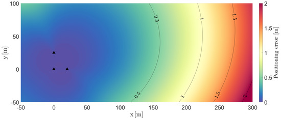
Figure 11.
Positioning error of a single swarm element based on the CRB with free-space path loss model. Black triangles show the anchor node positions and contour lines are plotted for every .
Let us look at the positioning error based on the CRB from (18) with the ranging variance determined by the CRB from (15) with the free-space path loss model. The CRB defined in (18) is the lower bound on the variance for and . The positioning error is, therefore, calculated as from (18). Figure 11 shows the result for the defined exploration area. We chose the geometry of the area such that we can investigate the positioning error close to the anchors, and further away where the geometry becomes unfavorable for precise positioning. Due to the free-space path loss assumption, we observe a smoothly increasing positioning error at a larger distance from the anchors. The positioning error reaches about 2 at a distance of 300 from the origin based on our system parameters.
The positioning error significantly increases with the two-ray ground reflection model for the ranging variance. Figure 12 shows the result, again based on the CRB. We can see rapid spatial variations in the positioning error and the maximum error reaches approx. 13 . The significantly increased positioning error at distances of around 230 and 115 result from the SNR drop at the receiver, leading to an increased ranging variance. See Figure 9 at similar horizontal distances for comparison.
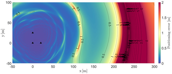
Figure 12.
Positioning error of a single swarm element based on the CRB with two-ray ground reflection model. Black triangles show the anchor node positions, and contour lines are plotted for every . The positioning error significantly increases and shows rapid spatial variations. The color coding is saturated at 2 , and errors of up to 13 are reached.
We now move from a CRB-based positioning variance prediction to an ML-based estimation defined in (29) and the evaluation of the positioning RMSE. First, we evaluated the correctness of the our ML estimation without ranging bias by comparing the resulting positioning RMSE with the CRB. In order to calculate the RMSE for each position, we use 1000 Monte-Carlo runs. For the final evaluation, we take the ranging bias from Section 3.2 into account. The distance estimate for the ML position estimator becomes
with as ranging bias, and the noise term . The ranging variance required for (29) is determined by (15) with the two-ray ground reflection model. At this point, we have to make clear that a model mismatch exists, as the weighting of distance estimates in the log-likelihood is solely based on the ranging variance. However, we are particularly interested in the resulting positioning RMSE, as a practically implemented positioning estimator is not aware of the ranging bias. The ranging variance can be determined by the SNR of the received signal. Figure 13 shows the final result. If we compare this result with Figure 12, we clearly see an increased positioning error in particular at smaller distances. At larger distances, we only see a minor increase in positioning error. This is expected as the ranging RMSE is dominated by the ranging bias for most distances; see Figure 9.
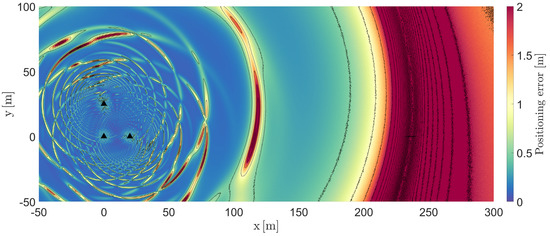
Figure 13.
Positioning error of a single swarm element based on ML estimation with the ranging bias and ranging variance determined by the two-ray ground reflection model. Black triangles show the anchor node positions and contour lines are plotted every . For visual clarity, we removed contour labels and the color-coding is saturated at 2 .
Based on the final result in Figure 13, we obtain the following three main conclusions. Firstly, the predicted positioning error is significantly larger with the two-ray ground reflection model, compared to the too-optimistic free-space path loss model. Secondly, the positioning CRB with the two-ray ground reflection model can provide insights as to which locations in the exploration area we cause us to experience an increased positioning error. Thirdly, if we assume a certain robot trajectory through the exploration area, the robot will experience a rapidly changing positioning error along the trajectory. This is in particular of interest for tracking applications, as, in this work, we focus on snapshot-based estimation.
6. Cooperative Positioning Performance
We now extend the scenario from non-cooperative positioning to cooperative positioning. We chose an identical setup as before, randomly place Q swarm elements in the defined area, calculate the cooperative positioning CRB, and estimate the swarm elements’ positions. For ML estimation, we use 1000 realizations for each of the randomly selected swarm-element positions. To evaluate the resulting overall positioning performance, we determine the CDF (cumulative distribution function) of the positioning RMSEs of all swarm elements.
Figure 14 shows the CDF of the positioning error for swarm-elements. The result, based on the CRB with the FSPL model, provides the reference. We can see that the estimator approaches the result obtained by the CRB; see the solid blue line. Interestingly, we obtain a lower positioning error based on the CRB with the two-ray ground reflection model. We identified this to be caused by the increased SNR due to the constructive superposition of the LoS signal component and the ground-reflected signal component. For example, in Figure 9 we see the peaks in increased ranging variance followed by a decreased ranging variance over the horizontal distance . The value range of with a smaller ranging variance is larger compared to the one for larger ranging variances. In this unbiased case, the two-ray ground reflection model, on average, is even beneficial for cooperative positioning. However, we also have to take the ranging bias into account and we model the distance estimate as input for the positioning estimator with (31) and with
The orange curve in Figure 14 shows the result of the estimator with the ranging bias, and the ranging variance determined by the two-ray ground reflection model. The positioning error is significantly increased: from 18 to 83 for the percentile.
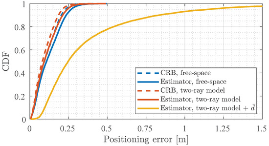
Figure 14.
CDF of the positioning error for swarm-elements. The CRB with free-space path loss provides the reference. The estimator approaches the CRB, and we see a significantly increased positioning error with the two-ray ground-reflection model and included ranging bias .
Next, we look at how the positioning error obtained from the estimator with the two-ray ground reflection model and ranging bias improves with an increasing number of swarm-elements Q. Figure 15 shows the CDF curve of the resulting positioning error. In the single-swarm-element scenario, we see a large positioning error; see also Figure 13. Adding a second swarm element for cooperative positioning reduces the overall positioning error significantly, as well as for swarm elements. Increasing the number of swarm elements even more improves the positioning error, as expected [17]. However, the improvement becomes minor, even though we assume a fully meshed network. This results from the ranging bias, which is not zero-mean, and thus does not spatially average out.
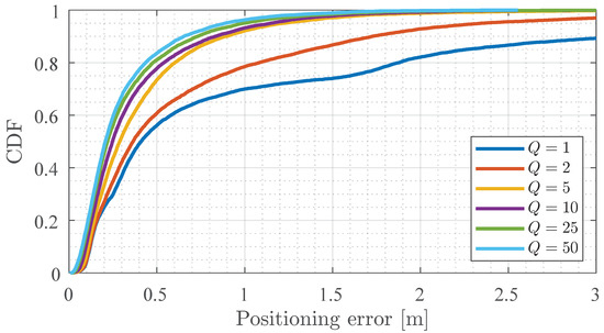
Figure 15.
CDF of the positioning error for an increasing number of Q swarm-elements. As expected, we see an improvement for increasing Q, but it becomes small beyond five swarm-elements.
Figure 16 shows the 90th percentile of the CDFs from Figure 15, with results from the estimator. The resulting 90th percentiles over Q more clearly show the gain obtained by cooperative positioning with multiple swarm elements. For all three models, the error is steadily decreasing. We are particularly interested in the positioning error with the two-ray ground reflection model with ranging bias . The percentile reduces from for to for . Beyond the five swarm elements, the percentile decrease is small.
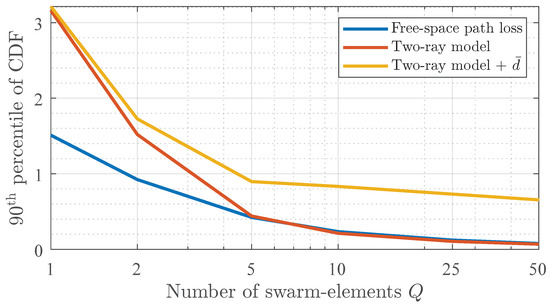
Figure 16.
90th percentile of the positioning error over the number of swarm elements Q. An increasing number of Q results in a lower positioning error in general. However, for the two-ray ground reflection model with ranging bias , the error decrease becomes small for .
Based on the results in this section, we can conclude with three important findings. Firstly, the overall positioning error with ranging variance and ranging bias determined by the two-ray ground reflection model is significantly larger compared to using the too-optimistic FSPL model. Secondly, an increasing number of swarm elements, cooperatively estimating their positions, improves the positioning performance. Thirdly, we do not necessarily need a large number of swarm elements to obtain an improved positioning performance compared to a single swarm element positioning: in our scenario, five swarm elements are sufficient. An even larger number of swarm elements does not improve the positioning error too much, as we are ranging-bias-limited. However, this is only strictly valid for our defined area, antenna heights, and the fully meshed network assumption. For larger areas with less well-connected swarm elements, and different antenna heights, a higher number of swarm elements will certainly improve the positioning performance.
7. Conclusions
In this work, we investigated the impact of a two-ray ground reflection model for ranging error determination on the cooperative positioning performance. In particular, we investigated the resulting ranging bias caused by the superposition of the LoS signal component and the signal component reflected from the ground. Based on the presented results, we draw the following conclusions. In general, the FSPL model is too optimistic to adequately assess the cooperative positioning performance. The two-ray ground reflection model without ranging bias determination provides a better assessment. However, the ranging RMSE is mostly dominated by the ranging bias and not the ranging variance. Thus, the ranging bias must be considered for a realistic performance assessment. Increasing the signal bandwidth and transmit power for ranging does not necessarily improve the ranging RMSE. The antenna heights are important, as the overall geometry has a significant influence on the fractional delay with respect to the signal sample length. Similar to existing works, we observe, on average, a lower positioning error for cooperative positioning with an increasing number of swarm elements. However, as the ranging bias is a limiting factor for large swarms, we do not see the same improvement as the simplistic FSPL model assumption. The positioning error shows spatially rapid variations with the two-ray ground reflection model for ranging. As a consequence, a position tracking algorithm must be properly designed to take this into account. Finally, resulting ranging biases and ranging variances are sensitive to the selected carrier frequency and relative geometry. The value of relative ground permittivity for a generally dry soil is less important.
8. Outlook
The investigations presented in this work stimulated many discussions among the authors, and the results provide the first insights and a fundamental base. As a next step, we will investigate different polarizations, such as horizontal and circular polarized radio waves. In addition, we assume that a fully meshed network ranging down to very low SNR values is possible. In practice, ranging requires communication as well; thus, the SNR must be high enough for correct decoding. This will result in a SNR threshold behaviour for a real OFDM receiver. Finally, terrain data representative of the lunar or Martian surface should be included.
Author Contributions
Conceptualization, E.S.; formal analysis, E.S. and R.P.; investigation, E.S., R.P., A.D. and S.Z.; methodology, E.S. and R.P., software, E.S. and A.D.; supervision, E.S.; visualization, E.S.; writing—original draft, E.S.; writing—review and editing, E.S., R.P., A.D. and S.Z. All authors have read and agreed to the published version of the manuscript.
Funding
This research received no external funding.
Conflicts of Interest
The authors declare no conflict of interest.
Abbreviations
The following abbreviations are used in this manuscript:
| 2D | two-dimensional. |
| 3D | three-dimensional. |
| BFGS | Broyden–Fletcher–Goldfarb–Shanno. |
| CDF | cumulative distribution function. |
| CIR | channel impulse response. |
| CRB | Cramér-Rao bound. |
| DLL | delay-locked loop. |
| FFT | fast Fourier transform. |
| FIM | Fisher information matrix. |
| FSPL | free-space path loss. |
| GNSS | global navigation satellite system. |
| IFFT | inverse fast Fourier transform. |
| LoS | line-of-sight. |
| MEE | multipath error envelope. |
| ML | maximum likelihood. |
| MSE | mean square error. |
| OFDM | orthogonal frequency-division multiplexing. |
| RMSE | root mean square error. |
| RTT | round trip time. |
| SNR | signal to noise ratio. |
| ToF | time of flight. |
| TWR | two-way ranging. |
References
- Andreescu, L. 100 Radical Innovation Breakthroughs for the Future; Technical Report KI-01-19-886-EN-N, European Commission-Directorate-General for Research and Innovation; 2019. Available online: https://op.europa.eu/en/publication-detail/-/publication/3e2e92d6-1647-11ea-8c1f-01aa75ed71a1/language-en (accessed on 27 February 2023).
- Abraham, L.; Biju, S.; Biju, F.; Jose, J.; Kalantri, R.; Rajguru, S. Swarm Robotics in Disaster Management. In Proceedings of the 2019 International Conference on Innovative Sustainable Computational Technologies (CISCT), Dehradun, India, 11–12 October 2019; pp. 1–5. [Google Scholar] [CrossRef]
- Wedler, A.; Wilde, M.; Dömel, A.; Müller, M.G.; Reill, J.; Schuster, M.; Stürzl, W.; Triebel, R.; Gmeiner, H.; Vodermayer, B.; et al. From Single Autonomous Robots toward Cooperative Robotic Interactions for Future Planetary Exploration Missions. In Proceedings of the International Astronautical Congress, IAC, Bremen, Germany, 1–5 October 2018. [Google Scholar]
- Zhang, S.; Pöhlmann, R.; Staudinger, E.; Dammann, A. Assembling a Swarm Navigation System: Communication, Localization, Sensing and Control. In Proceedings of the 2021 IEEE 18th Annual Consumer Communications Networking Conference (CCNC), Las Vegas, NV, USA, 9–12 January 2021; pp. 1–9. [Google Scholar] [CrossRef]
- Global Exploration Roadmap, Supplement August 2020, Lunar Surface Exploration Scenario Update; Technical Report NP-2020-07-2888-HQ; International Space Exploration Coordination Group: 2020. Available online: https://www.globalspaceexploration.org/wp-content/uploads/2020/08/GER_2020_supplement.pdf (accessed on 27 February 2023).
- NASA’s Lunar Exploration Program Overview; Technical Report NP-2020-05-2853-HQ; International Space Exploration Coordination Group: 2020. Available online: https://www.nasa.gov/sites/default/files/atoms/files/artemis_plan-20200921.pdf (accessed on 27 February 2023).
- Zhang, S.; Pöhlmann, R.; Wiedemann, T.; Dammann, A.; Wymmeersch, H.; Hoeher, P.A. Self-Aware Swarm Navigation in Autonomous Exploration Missions. Proc. IEEE 2020, 108, 1168–1195. [Google Scholar] [CrossRef]
- Vassev, E.; Sterritt, R.; Rouff, C.; Hinchey, M. Swarm Technology at NASA: Building Resilient Systems. IT Prof. 2012, 14, 36–42. [Google Scholar] [CrossRef]
- Wiedemann, T.; Shutin, D.; Lilienthal, A.J. Model-based gas source localization strategy for a cooperative multi-robot system—A probabilistic approach and experimental validation incorporating physical knowledge and model uncertainties. Rob. Auton. Syst. 2019, 118, 66–79. [Google Scholar] [CrossRef]
- Zhang, S.; Staudinger, E.; Pöhlmann, R.; Dammann, A. Cooperative Communication, Localization, Sensing and Control for Autonomous Robotic Networks. In Proceedings of the IEEE International Conference on Autonomous Systems (IEEE ICAS 2021), Montreal, QC, Canada, 11–13 August 2021. [Google Scholar]
- Dardari, D.; Conti, A.; Ferner, U.; Giorgetti, A.; Win, M.Z. Ranging With Ultrawide Bandwidth Signals in Multipath Environments. Proc. IEEE 2009, 97, 404–426. [Google Scholar] [CrossRef]
- Wymeersch, H.; Lien, J.; Win, M. Cooperative Localization in Wireless Networks. Proc. IEEE 2009, 97, 427–450. [Google Scholar] [CrossRef]
- Buehrer, R.M.; Wymeersch, H.; Vaghefi, R.M. Collaborative Sensor Network Localization: Algorithms and Practical Issues. Proc. IEEE 2018, 106, 1089–1114. [Google Scholar] [CrossRef]
- Zhang, S.; Staudinger, E.; Sand, S.; Raulefs, R.; Dammann, A. Anchor-Free Localization using Round-Trip Delay Measurements for Martian Swarm Exploration. In Proceedings of the IEEE ION PLANS, Monterey, CA, USA, 5–8 May 2014. [Google Scholar]
- Staudinger, E.; Zhang, S.; Poehlmann, R.; Dammann, A. The Role of Time in a Robotic Swarm: A Joint View on Communications, Localization, and Sensing. IEEE Commun. Mag. 2021, 59, 98–104. [Google Scholar] [CrossRef]
- Shen, Y.; Win, M.Z. Fundamental Limits of Wideband Localization— Part I: A General Framework. IEEE Trans. Inf. Theory 2010, 56, 4956–4980. [Google Scholar] [CrossRef]
- Shen, Y.; Wymeersch, H.; Win, M. Fundamental Limits of Wideband Localization, Part II: Cooperative Networks. IEEE Trans. Inf. Theory 2010, 56, 4981–5000. [Google Scholar] [CrossRef]
- Van Trees, H.L. Detection, Estimation, and Modulation Theory; John Wiley and Sons, Ltd.: Hoboken, NJ, USA, 2001; Chapter 2; pp. 19–165. [Google Scholar] [CrossRef]
- Wedler, A.; Müller, M.G.; Schuster, M.J.; Durner, M.; Lehner, P.; Dömel, A.; Vayugundla, M.; Steidle, F.; Sakagami, R.; Meyer, L.; et al. Finally! Insights into the ARCHES Lunar Planetary Exploration Analogue Campaign on Etna in Summer 2022. In Proceedings of the International Astronautical Congress (IAC). International Astronautical Federation, Naples, Italy, 1–5 October 2012. [Google Scholar]
- Pöhlmann, R.; Staudinger, E.; Zhang, S.; Dammann, A. Simultaneous Localization and Calibration for Radio Navigation on the Moon: Results from an Analogue Mission. In Proceedings of the ION GNSS+ 2022, Denver, CO, USA, 19–23 September 2022. [Google Scholar]
- Rappaport, T.S. Wireless Communications—Principles and Practice; Prentice Hall: Saddle River, NJ, USA, 1996; pp. I–XVI, 1–641. [Google Scholar]
- Santra, S.; Paet, L.B.; Staudinger, E.; Yoshida, K. Radio Propagation Modelling for Coordination of Lunar Micro-Rovers. In Proceedings of the International Symposium on Artificial Intelligence, Robotics and Automation in Space (i-SAIRAS). Lunar and Planetary Institute, Universities Space Research Association, Pasadena, CA, USA, 18–21 October 2020; pp. 1–8. [Google Scholar]
- Staudinger, E.; Walter, M.; Dammann, A. The 5G Localization Waveform Ranging Accuracy over Time-Dispersive Channels—An Evaluation. In Proceedings of the ION-GNSS, Portland, Oregon, 12–16 September 2016. [Google Scholar]
- Siegler, M.A.; Feng, J.; Lucey, P.G.; Ghent, R.R.; Hayne, P.O.; White, M.N. Lunar Titanium and Frequency-Dependent Microwave Loss Tangent as Constrained by the Chang’E-2 MRM and LRO Diviner Lunar Radiometers. J. Geophys. Res. Planets 2020, 125, e2020JE006405. [Google Scholar] [CrossRef]
- Dielectric properties estimation of the lunar regolith at CE-3 landing site using lunar penetrating radar data. Icarus 2017, 284, 424–430. [CrossRef]
- Lai, J.; Xu, Y.; Zhang, X.; Xiao, L.; Yan, Q.; Meng, X.; Zhou, B.; Dong, Z.; Zhao, D. Comparison of Dielectric Properties and Structure of Lunar Regolith at Chang’e-3 and Chang’e-4 Landing Sites Revealed by Ground-Penetrating Radar. Geophys. Res. Lett. 2019, 46, 12783–12793. [Google Scholar] [CrossRef]
- Oguchi, T.; Udagawa, M.; Nanba, N.; Maki, M.; Ishimine, Y. Measurements of Dielectric Constant of Volcanic Ash Erupted From Five Volcanoes in Japan. IEEE Trans. Geosci. Remote. Sens. 2009, 47, 1089–1096. [Google Scholar] [CrossRef]
- Electrical Characteristics of the Surface of the Earth; Technical Report Recommendation ITU-R P.527-4, International Telecommunication Union (ITU-R); ITU: Geneva, Switzerland, 2017.
- Van Trees, H.L.; Bell, K.L. Bayesian Bounds for Parameter Estimation and Nonlinear Filtering/Tracking; John Wiley IEEE Press: Hoboken, NJ, USA, 2007. Available online: https://pubs.aip.org/asa/jasa/article/123/5/2459/932358/Bayesian-Bounds-for-Parameter-Estimation-and (accessed on 27 February 2023).


Disclaimer/Publisher’s Note: The statements, opinions and data contained in all publications are solely those of the individual author(s) and contributor(s) and not of MDPI and/or the editor(s). MDPI and/or the editor(s) disclaim responsibility for any injury to people or property resulting from any ideas, methods, instructions or products referred to in the content. |
© 2023 by the authors. Licensee MDPI, Basel, Switzerland. This article is an open access article distributed under the terms and conditions of the Creative Commons Attribution (CC BY) license (https://creativecommons.org/licenses/by/4.0/).