Abstract
Time delay estimation (TDE) is of great interest for the thickness estimation of pavement using ground penetrating radar (a non-destructive testing tool that uses electromagnetic waves to probe civil engineering material), which determines the difference between the times of arrival of two incoming signals or backscattered echoes. However, conventional TDE methods suffer performance degradation because of limited resolution for thin layers and highly correlated backscattered echoes. In this paper, a deep neural network (DNN)-based TDE method is proposed. Firstly, a new DNN is constructed to classify and train the backscattered echoes; then, the time delays of the backscattered echoes can be estimated through the proposed DNN. The proposed method is based on the data processing of the backscattered echoes, which is more robust to the noise than conventional subspace-based methods (MUSIC, ESPRIT) and compressive sensing-based methods (OMP). The proposed method can directly process coherent backscattered echoes without decorrelation procedures, compared with MUSIC and ESPRIT. In addition, the proposed method is more powerful in resolving the close backscattered echoes than that of OMP. Simulation results show the efficiency of the proposed method in terms of signal-to-noise ratio (SNR) and products. (The products indicate the resolution of GPR, B is the frequency bandwidth of GPR and is the time delay between two incoming signals or backscattered echoes).
1. Introduction
Ground-penetrating radar (GPR) is a useful tool for non-destructive testing that uses electromagnetic (EM) waves to probe objects of civil engineering material, such as pavements [1,2,3], buildings [4] and bridges [5]. In this paper, we focus on the application of GPR in pavement thickness estimation. During road pavement surveys, with the purpose of measuring the thickness of different layers, the road layers are supposed to be horizontally stratified. The vertical structure of road pavement can be deduced by means of echo detection and amplitude estimation. The time delay estimation (TDE) associated with each interface is provided by echo detection, which is of great importance when measuring the thickness of different layers of pavement.
TDE is an important parameter for estimating pavement thickness using GPR. However, conventional TDE methods such as FFT-based methods and beamforming-based methods have difficulty in distinguishing close (overlapped) backscattered echoes (where , B is the frequency bandwidth of GPR, is the time delay between two echoes). High-resolution methods, for example, multiple signal classification (MUSIC) [6] and estimation of signal parameters via rotational invariance techniques (ESPRIT) [7], have infinite time resolution in theory and cannot handle the high correlated or coherent backscattered echoes due to the rank loss in the source covariance matrix. Decorrelation methods are needed to decorrelate the correlation between echoes. The classical decorrelation method, spatial smoothing preprocessing (SSP), was first proposed in [8] and later modified in [9] called modified SSP (MSSP), which partitions the entire frequency band into a series of overlapping sub-bands to obtain a new data covariance matrix with restored rank. Many improvements based on SSP have been proposed [10,11,12].
Moreover, compressive sensing (CS)-based methods have also been proposed for TDE by GPR, which can solve the issue of the highly correlated or coherent backscattered echoes without decorrelating. The matching pursuit (MP) and orthogonal matching pursuit (OMP) are the two most popular classical greedy algorithms for sparse reconstruction, which can be used for TDE [13]. However, these two methods cannot handle overlapped echoes () due to limited resolution.
Machine learning and deep learning methods have widely been used by researchers as crucial tools to process GPR signals over the past decade, which are especially widely used in GPR image processing. In contrast, techniques that used deep learning work directly on GPR data rather than radar data models, and they do not require high-precision GPR devices and effective feature extractors. These methods reduce the processing time of received GPR signals and revolutionize several classification and regressing tasks [14,15,16]. Cao et al. [14] adopt a novel deep residual network called Mois-ResNets to predict the internal moisture content of AC pavement from GPR. Zhang et al. [15] propose a CNN model to detect moisture damage areas from GPR B-scans. Tong et al. [16] adopt NiN to measure pavement defects using GPR A-scan. Although those deep learning-based methods have shown great advantages in road infrastructure monitoring, they still need further investigation regarding estimating the thin pavement thickness, of which the difficulty lies in distinguishing backscattered echoes. It is of great significance to combine deep learning methods with TDE of backscattered echoes using GPR.
This paper utilizes deep learning to perform TDE of backscattered echoes and incorporates the autoencoder into the deep learning network (DNN) architecture model [17]. The multitask autoencoder can be used for feature extraction, denoising, and dimensionality reduction, among others. The multitask autoencoder can learn more robust and generalizable representations of the input data by incorporating multiple tasks into a single neural network architecture. The proposed method effectively solves the problem of estimation accuracy of traditional ground-penetrating radar signal processing algorithms caused by a low signal-to-noise ratio (SNR) and overlapped echoes, enabling the estimation result with high accuracy and reliability.
The merits of the proposed method on TDE directly contribute to thickness estimation, especially for thin layers (overlapped echoes). The proposed method can also be used to infer the dielectric properties and the position of buried objects.
2. Radar Data Model
For road pavements probed under GPR vertical incidence, it is often a horizontally layered medium. In road condition detection engineering, we generally focus on the first two or three top layers of the road medium, which are composed of smooth and homogeneous layers with low dielectric constants and negligible conductivity, and each layer of the medium generates only one echo signal during detection. Based on this application context, for horizontally layered lossless media, the receiver-side radar signal model can be expressed as [18]:
where K is the number of backscattered echoes, is radar pulses in the frequency domains, denotes the amplitude of the kth backscattered echo; is additive Gaussian white noise, and the mean and variance of the noise are 0 and ; frequency samples , where represents the lowest frequency in the studied band and is the frequency shift, .
The above equation can be written in the following vector form:
where
- is the received signal vector, with the superscript T denoting the transpose of the matrix.;
- is an diagonal matrix whose diagonal elements are the radar pulses in the frequency domain;
- is the mode matrix, with ;
- is a vector of echoes’ amplitudes;
- is the noise vector.
Assuming that the additional noise is independent of the echo, the covariance matrix of the received signal can be written as
where E(·) denotes the ensemble average, denotes the covariance matrix of the vector s, and denotes the identity matrix and is the covariance matrix.
3. Neural Network Models
3.1. Training Dataset Structure
To reduce the significant influence of uncertain signal waveforms when training DNN, we follow the guidelines mentioned in [19] to calculate and process the covariance matrix after obtaining it according to (3). Since the main diagonal elements of do not contain time delay information and the covariance matrix is symmetric, we reformulate the non-diagonal upper right matrix elements as DNN input vector for the overall network architecture, and the non-diagonal upper right matrix elements of the covariance matrix also need to be vectorized. The overall implementation framework for preprocessing the incoming data is shown in Figure 1.
where and can be obtained from (4) and (5), respectively. denotes the th element of the covariance matrix, and denote taking the real and imaginary parts of the complex tensor in order, respectively, and denotes taking the two-parametric numbers. The output obtained after preprocessing is the result of normalization, which is a vector of dimension .
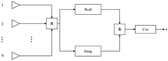
Figure 1.
General implementation framework for the preprocessing of the dataset.
3.2. Overall Network Design Framework
The overall network architecture model is shown in Figure 2, which contains two main modules: one module is a multitask autoencoder with spatial filtering function and the other module is a classifier consisting of a set of deep neural networks that are independent of each other.
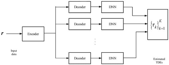
Figure 2.
Overall network architecture model based on the DNN neural network approach.
The multitask autoencoder acts as a spatial filter, which performs noise reduction on the actual received signal and decomposes the signal components into several spatial sub-regions. When the received signal is fed into the network, if the real value of the time delay parameter of the actual signal exists in one of the spatial sub-regions, the output of the decoder is equal to the input to the network, and the output of the decoder corresponding to other sub-regions are set to zero.
The method proposed possesses a better classification performance of the backscattered echoes. By means of the autoencoder structure, the subsequent classifiers are trained with a more focused distribution of parameters, improving the generalization ability of this network to unknown scenes and signals, which allows us to estimate the time delay of multiple targets more effectively while reducing the difficulty of training.
3.3. Multitask Autoencoder
Assuming that the multitask autoencoder divides the signal into V sub-regions. The input of the network is a one-dimensional vector. The multi-tasking encoder extracts the feature components of the original input data and compresses them to a lower dimensional vector, followed by V multi-tasking decoders that process the vector obtained with a different decoder and restore the data to its original dimension. In other words, the signal data at the output of each decoder is of the same dimension as the original data at the input encoder. This module is designed to reduce the effects of noise and signal interference in the input signal [20].
The multitask autoencoder is a neural network that consists of fully connected nodes in adjacent layers, and the output dimension of each layer of the encoder decreases as the number of network layers increases, while the output dimension of each decoder increases as the number of network layers increases. is the number of network layers for the encoder and decoder, and in general, the output dimension of the encoder at the th layer is the same size as the output dimension of the decoder at the th layer, where . This symmetry in layer dimensions helps ensure that the encoded representation can be easily decoded back into the original input.
For the multitask autoencoder module, the relationship between the output data of the two adjacent layers can be expressed as
where denotes the original input data of the overall network, denotes the th output layer of the autoencoder, denotes the feed-forward weight matrix between the th layer and the th layer, whose dimension depends on the size of the network architecture model of the preceding and following layers, denotes the additive bias vector of the th layer, and denotes the activation function. In order to ensure that the designed autoencoder module can be practically applied to the TDE of multiple GPR backscattered echoes, the multitask autoencoder should achieve the decomposition of input vectors to different decoder outputs in turn. The system should be addictive, ensuring that all echoes are located in the correct sub-regions. To ensure that the designed multitask autoencoder system satisfies linearity, the unit function is substituted for the non-linear activation function, serving as for the activation function . Both encoders and decoders from different sub-regions satisfy the relationship above.
Based on the previous theoretical analysis, the time delay value which corresponds to the received backscattered echo is , which is located in the mth decoder of the multitasking autoencoder. The input of the autoencoder after signal preprocessing is and the overall output of the encoder can be obtained as
During the training process, the time delay value corresponding to the received backscattered echoes is traversed throughout the interval of values of the time parameter, and a set of vectors of dimension obtained after the preprocessing step of the data is the dataset for the multitask autoencoder training, as is shown in (5). The corresponding label set can be obtained from Equation (7), and the above data set and the label set form a set of data label pairs for the autoencoder training. Equation (8) is the loss function for training the autoencoder, and the formula is the actual output of the autoencoder.
After calculating the loss function, the back-propagation gradient of the loss function with respect to the variables can be used to update the weights and biases [17].
3.4. Multi-Layer Classifier
After multitasking, the data is divided into V sub-regions and fed into the multi-layer classifier. The functions of this module include refining the antecedent sub-regions into more accurate grid points, obtaining highly accurate delay estimates and enabling multi-signal delay estimation, satisfying the requirements of changing SNR and handling overlapped echoes.
The second module consists of several deep neural networks. These networks, existing in each spatial sub-region, are independent of each other. Each network functions as a refinement of the entire interval of the time delay of interest in a grid-like form. The DNN on each sub-region functionally behaves as a classifier, and each network computes and processes the data in a feed-forward manner. The signal located on a grid point or between two grid points corresponds to a non-zero value at the network node, while the remaining grid points correspond to a zero value at the output, and the value at the number of nodes represents the proximity of the time delay to the grid point.
Figure 3 shows a schematic of a fully connected DNN for TDE.
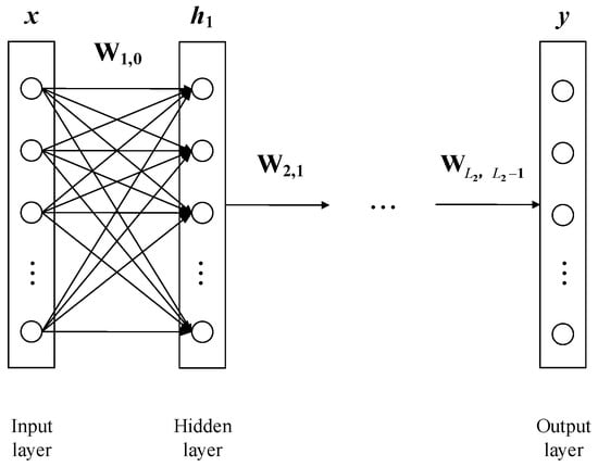
Figure 3.
Schematic of a fully connected DNN for TDE.
In Figure 3, is the input of the current classifier, which is connected to the multitask autoencoder, and , is the output vector of the th hidden layer and represents the output of the current classifier. Since in the context of ground-penetrating radar applications, echo signals with close time intervals will have a more similar vector form when received, it is necessary to introduce a non-linear activation function to respond to the non-linear characteristics of the signal in order to better differentiate them, so a non-linear activation layer is added to the output of each layer of the network and the relationship between the output data of two adjacent hidden layers is shown as
where is the number of network layers of the encoder and decoder, denotes the feed-forward weight matrix of the network at the th layer, denotes the additive bias vector at the th layer, and denotes the non-linear activation function of the hidden layer. In order to reflect the non-linear characteristics of the input data and maintain the polarity of each layer of the classifier, as for , the hyperbolic tangent function is chosen in this paper, and its expression is shown as
Finally, the outputs of all classifiers are combined and then vectorized, with the final data dimension being the same as the number of grid points, which is related to the accuracy and range of the time delay parameter. In order to be able to implement the TDE estimation function based on the spectral signal, only the grid nodes corresponding closely to the true time delay value of the signal end up with positive values, the values of all the rest of the grid nodes are expected to be zero.
The module is also capable of estimating the delay of multiple signals. In addition, the training of this module is carried out separately from the training of the preceding encoder–decoder network module, i.e., the weights and biases of the preceding network are saved for the training of the parallel classifier. Therefore, in this module, we need to obtain another training dataset with two simultaneous GPR backscattered echoes.
Assuming that one of the time delays of the echo reflection signal is and is a certain time interval value sampled, the time delay of another signal can be expressed as , and the corresponding input of the encoder input is , then the whole of the desired DNN network output can be expressed as
where correspond to the two grid points closest to the true value of the current time delay estimate. It is theoretically possible to make the output of the classifier have only the grid points corresponding to the true time delay signal, or the grid points adjacent to it with non-zero values, and the relative magnitude of the values determines the size of the estimated time delay, achieving a more accurate estimation of the echo signal. Equation (12) is the loss function for training the classifier, and is the actual output of the DNN network. After calculating the loss function, the back-propagation gradient of the loss function relative to the variables can be used to update the weights and biases.
The following steps summarize the DNN-based TDE method:
After the whole network is designed and trained, the weights and biases of the network are saved. The TDE of GPR backscattered echoes can be obtained after presenting the input vector to the network.
4. Simulation Analysis
In this section, the proposed method is tested on a pavement made up of three layers (Figure 4), the first layer is the air and the second and third layers are asphalt surfacing, whose relative permittivities are and , respectively. The thickness of the second layer (H) is approximately 28 mm. Therefore, the times of arrival of the backscattered echoes from the second layer () are 1.1 ns and 1.5 ns, respectively. In the simulation, the frequency band is 1.0–3.0 GHz ( GHz) with a step size of GHz (11 frequency samples in total). The statistical performance of the proposed method is compared with MUSIC, ESPRIT and OMP. For the subspace-based methods MUSIC and ESPRIT, MSSP is applied to decorrelate the correlation between highly correlated echoes with the number of sub-bands equal to 6 [12].
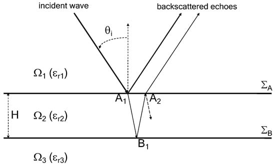
Figure 4.
The pavement configuration.
In the following, the performance of the proposed method is evaluated with a Monte-Carlo process of 100 independent runs of the method from the relative root mean square error (RRMSE) of the estimated parameters. The expression of RRMSE is shown as
where denotes the estimated parameter of the jth run of the method, z denotes the true value of the parameter, and Q denotes the number of Monte-Carlo processes. The parameter z can be referred to as the time delay of backscattered echoes. The simulation parameters are set as follows:
The vectors in the training dataset for both the autoencoder and classifier modules were obtained with 500 independent snapshots. SNR is defined as the ratio between the power of the second backscattered echo and the noise variance. The number of sub-regions divided into four after the multi-task auto-encoder consists of a grid with 0.1 ns intervals, with a delay parameter ranging from 0.5 to 2.5 ns and a total number of grid points , with five grid points per sub-region. The covariance vector and the corresponding label are calculated separately for each time delay based on (5) and (7), and only one set of snapshots is collected to calculate a covariance vector on each grid of time parameters. A small batch training method [21] was used, with batch size set to 16, learning rate set to and epoch size set to 300.
The parameters of the multitask autoencoder network architecture are as follows.
- (1)
- The size of the input layer is , where .
- (2)
- The size of the hidden layer is .
- (3)
- The size of the output layer is , where .
Once the autoencoder has been trained, the weight matrix of this module is fixed and another dataset is trained for the classifier. As for the dataset to be trained, the time interval is sampled from ns. For the model of two GPR backscattered echoes, the time delay of the first signal is sampled from 0.5 ns to ns, which is denoted by , and the time delay of the second signal , for each set of time parameters corresponding to the echo signal superimposed on the noise generated. The number of covariance vectors in the dataset for training is , while for validation, and 100 certain covariance vectors for testing.
For a single classifier, the network architecture parameters are as follows:
- (1)
- The size of the input layer is 110.
- (2)
- The sizes of the three hidden layers are 60, 30, and 10, respectively.
- (3)
- The size of the output layer is 5.
In the first simulation, the performance of the proposed method is tested with respect to noise. The RRMSE on the estimated value of is calculated and the SNR varies from to 10 dB.
It can be seen from Figure 5 that the RRMSE is continuously decreasing with the increase in SNR. The proposed method can accurately estimate the time delay of backscattered echoes with smaller RRMSE than its competitors within the tested SNR scenarios. The proposed DNN framework adapts well to noisy training data and possesses a better generalization ability.
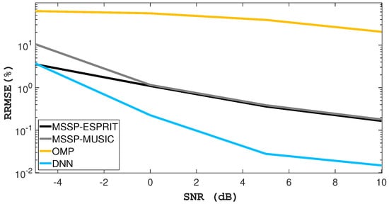
Figure 5.
RRMSE versus SNR.
In the second simulation, the resolution power of the proposed method is evaluated by using the product. The RRMSEs on the estimated time delay versus the product are calculated. The SNR is fixed at 0 dB, changes from ns to ns and the rest of the simulation parameters are the same as those of the first simulation.
It can be seen from Figure 6 when the product is small, that both the proposed method and its competitors fail to estimate the time delay due to limited resolution. With the increase in the (≥0.4) product, the proposed method can successfully distinguish two close backscattered echoes. The proposed method outperforms MSSP-MUSIC, MSSP-ESPRIT and OMP with smaller RRMSE in TDE for both non-overlapped and overlapped echoes.
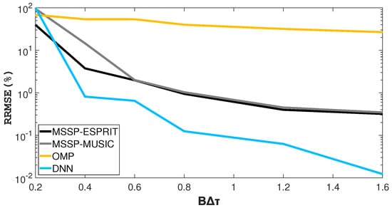
Figure 6.
RRMSE versus product.
In addition, when the product is small, the proposed method suffers performance degradation because of the loss of precision in the deep networks. This problem may be solved by increasing the number of units in various network layers, especially the size of the output.
5. Conclusions
This paper presents a deep learning-based method for TDE of GPR in pavement surveys. The proposed method constructs a deep neural network to classify and train the backscattered echoes, the time delays can then be estimated. The proposed method outperforms conventional MUSIC, ESPRIT and OMP in TDE, with different SNR and products. However, the number of samples required for the dataset is large when estimating time delays of multiple backscattered echoes. Therefore, future work will focus on a gridless TDE based on unsupervised deep learning to avoid the oversized dataset for training. In addition, the proposed method will be tested on real data to strengthen the results.
Author Contributions
Methodology, S.M.; Validation, F.L., S.M. and B.W.; Writing—original draft, F.L.; Writing—review & editing, M.S.; Supervision, M.S. All authors have read and agreed to the published version of the manuscript.
Funding
This research received no external funding.
Conflicts of Interest
The authors declare no conflict of interest.
References
- Benedetto, A.; Tosti, F.; Ciampoli, L.B.; D’Amico, F. An overview of ground-penetrating radar signal processing techniques for road inspections. Signal Process. 2017, 132, 201–209. [Google Scholar] [CrossRef]
- Le Bastard, C.; Baltazart, V.; Wang, Y.; Saillard, J. Thin-pavement thickness estimation using gpr with high-resolution and superresolution methods. IEEE Trans. Geosci. Remote Sens. 2007, 45, 2511–2519. [Google Scholar] [CrossRef]
- Annan, A.P.; Diamanti, N.; Redman, J.D.; Jackson, S.R. Ground-penetrating radar for assessing winter roads. Geophysics 2015, 81, WA101–WA109. [Google Scholar] [CrossRef]
- Chahine, K.; Baltazart, V.; Wang, Y. Interpolation-based matrix pencil method for parameter estimation of dispersive media in civil engineering. Signal Process. 2010, 90, 2567–2580. [Google Scholar] [CrossRef]
- Solla, M.; Asorey-Cacheda, R.; Núñez-Nieto, X.; Conde-Carnero, B. Evaluation of historical bridges through recreation of GPR models with the FDTD algorithm. NDT E Int. 2016, 77, 19–27. [Google Scholar] [CrossRef]
- Kim, J.M.; Lee, O.K.; Ye, J.C. Compressive MUSIC: Revisiting the link between compressive sensing and array signal processing. IEEE Trans. Inf. Theory 2012, 58, 278–301. [Google Scholar] [CrossRef]
- Qian, C.; Huang, L.; So, H.C. Computationally efficient ESPRIT algorithm for direction-of-arrival estimation based on Nyström method. Signal Process. 2014, 94, 74–80. [Google Scholar] [CrossRef]
- Evans, J.E.; Sun, D.; Johnson, J.R. Application of Advanced Signal Processing Techniques to Angle of Arrival Estimation in A TC Navigation and Surveillance Systems. Calculation. 1982. Available online: https://archive.ll.mit.edu/mission/aviation/publications/publication-files/technical_reports/Evans_1982_TR-582_WW-18359.pdf (accessed on 23 March 2023).
- Pillai, S.U.; Kwon, B.H. Forward/backward spatial smoothing techniques for coherent signal identification. IEEE Trans. Acoust. Speech Signal Process. 1989, 37, 8–15. [Google Scholar] [CrossRef]
- Qu, L.; Sun, Q.; Yang, T. Time-Delay Estimation for Ground Penetrating Radar Using ESPRIT with Improved Spatial Smoothing Technique. IEEE Geosci. Remote Sens. Lett. 2014, 11, 1315–1319. [Google Scholar]
- Sun, M.; Bastard, C.L.; Wang, Y.; Pinel, N. Time-delay estimation using ESPRIT with extended improved spatial smoothing techniques for radar signals. IEEE Geosci. Remote Sens. Lett. 2016, 13, 73–77. [Google Scholar] [CrossRef]
- Pan, J.; Sun, M.; Wang, Y. An enhanced spatial smoothing technique with ESPRIT algorithm for direction of arrival estimation in coherent scenarios. IEEE Trans. Signal Process. 2020, 68, 3635–3643. [Google Scholar] [CrossRef]
- Pan, J.; Sun, M.; Wang, Y.; Bastard, C.L.; Baltazart, V. Time-Delay Estimation by a Modified Orthogonal Matching Pursuit Method for Rough Pavement. IEEE Trans. Geosci. Remote Sens. 2021, 59, 2973–2981. [Google Scholar] [CrossRef]
- Cao, Q.; Al-Qadi, I.L.; Abufares, L. Pavement Moisture Content Prediction: A Deep Residual Neural Network Approach for Analyzing Ground Penetrating Radar. IEEE Trans. Geosci. Remote Sens. 2022, 60, 1–11. [Google Scholar] [CrossRef]
- Zhang, J.; Yang, X.; Li, W.; Zhang, S.; Jia, Y. Automatic detection of moisture damages in asphalt pavements from GPR data with deep CNN and IRS method. Autom. Construct. 2020, 113, 103119. [Google Scholar] [CrossRef]
- Tong, Z.; Yuan, D.; Gao, J.; Wei, Y.; Dou, H. Pavement-distress detection using ground-penetrating radar and network in networks. Construct. Build. Mater. 2020, 233, 117352. [Google Scholar] [CrossRef]
- Liu, Z.; Zhang, C.; Yu, P. Direction-of-Arrival Estimation Based on Deep Neural Networks With Robustness to Array Imperfections. IEEE Trans. Antennas Propag. 2018, 66, 7315–7327. [Google Scholar] [CrossRef]
- Sun, M.; Pan, J.; Bastard, C.L.; Wang, Y.; Li, J. Advanced Signal Processing Methods for Ground-Penetrating Radar: Applications to civil engineering. IEEE Signal Process. Mag. 2019, 36, 74–84. [Google Scholar] [CrossRef]
- Zooghby, A.; Christodoulou, C.G. A neural network-based smart antenna for multiple source tracking. IEEE Trans. Antennas Propag. 2000, 48, 768–776. [Google Scholar] [CrossRef]
- Hinton, G.E.; Salakhutdinov, R.R. Reducing the dimensionality of data with neural networks. Science 2006, 313, 504–507. [Google Scholar] [CrossRef] [PubMed]
- Huang, H.; Yang, J.; Song, Y.; Huang, H.; Gui, G. Deep Learning for Super-Resolution Channel Estimation and DOA Estimation Based Massive MIMO System. IEEE Trans. Veh. Technol. 2018, 67, 8549–8560. [Google Scholar] [CrossRef]
Disclaimer/Publisher’s Note: The statements, opinions and data contained in all publications are solely those of the individual author(s) and contributor(s) and not of MDPI and/or the editor(s). MDPI and/or the editor(s) disclaim responsibility for any injury to people or property resulting from any ideas, methods, instructions or products referred to in the content. |
© 2023 by the authors. Licensee MDPI, Basel, Switzerland. This article is an open access article distributed under the terms and conditions of the Creative Commons Attribution (CC BY) license (https://creativecommons.org/licenses/by/4.0/).