
A New Control for Improving the Power Quality Generated by a Three-Level T-Type Inverter
 , ,
, ,  ,
, 
Abstract
1. Introduction
- Minimizing the THD value of the current;
- Increasing the durability of the filtration system;
- Improving the dynamic response of the filtering system;
- Improving the power quality under unbalanced and distorted voltage conditions.
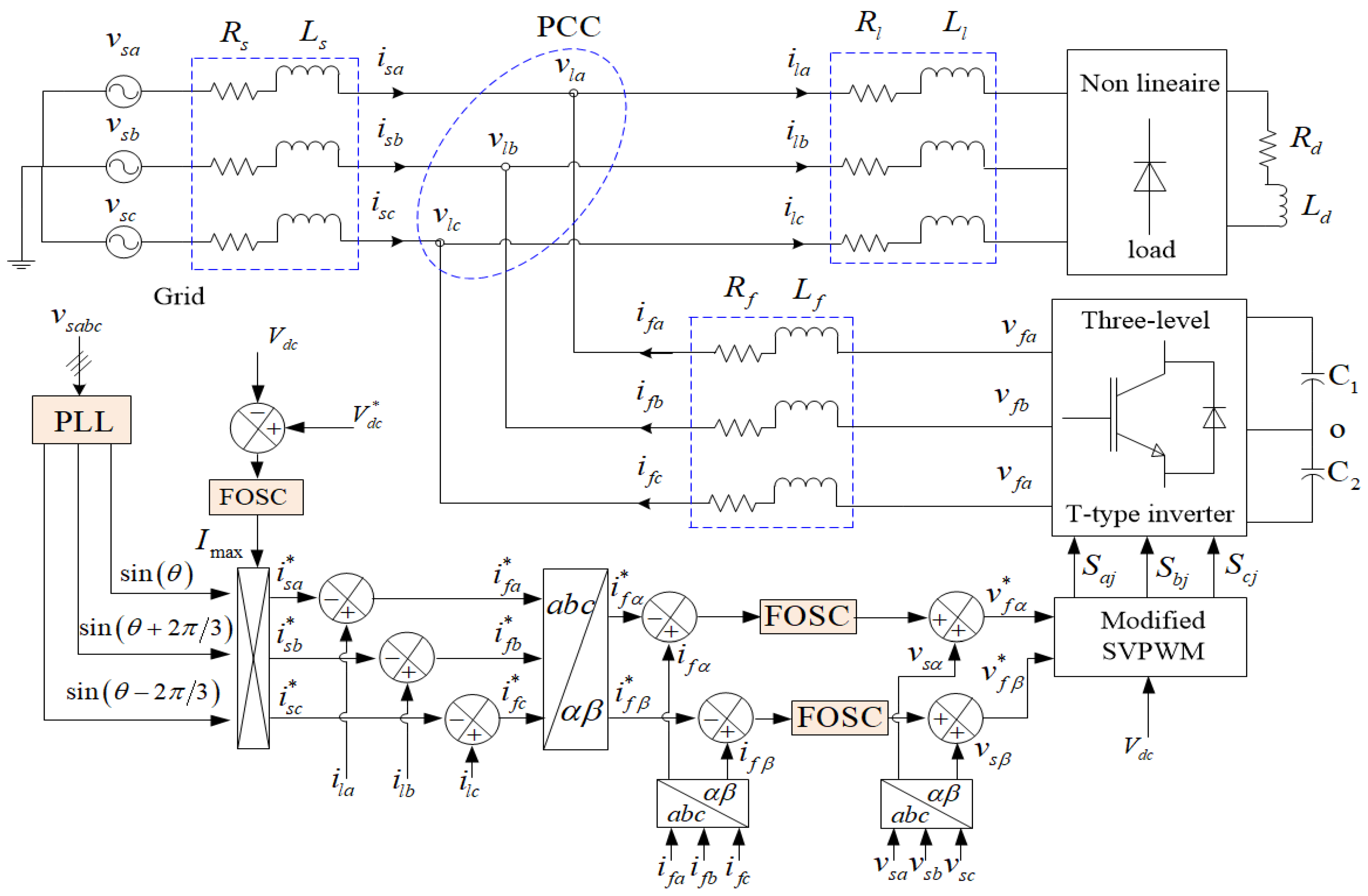
2. SAPF Configuration and Control
2.1. PLL-Based STF Technique
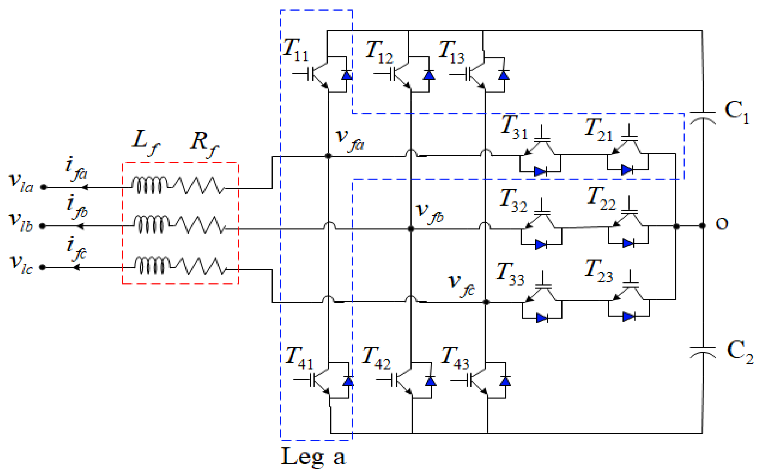
2.2. 3-Level T-Type Inverter
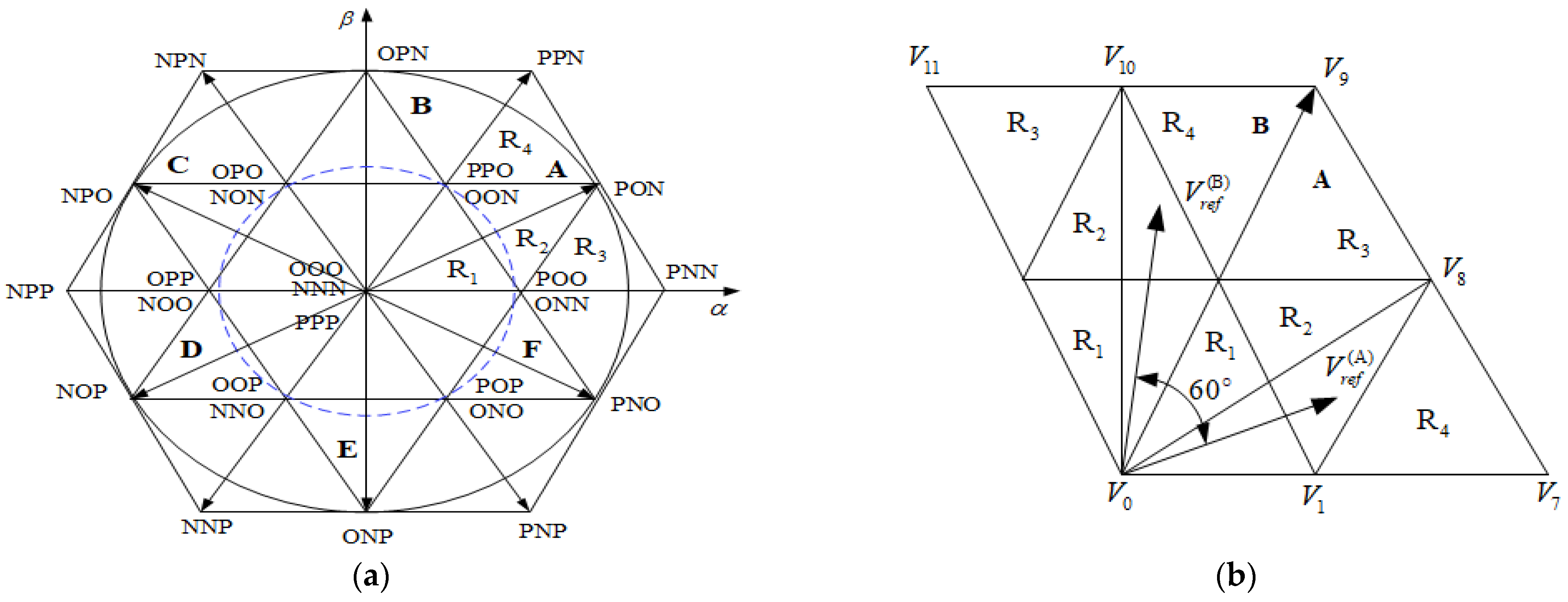
3. Control Strategy
3.1. Fractional Differentiation and Integration
- The initial time is taken to be zero.
- The Riemann-Liouville fractional derivative of order as:
3.2. SC Design
4. Fractional-Order Synergetic Control
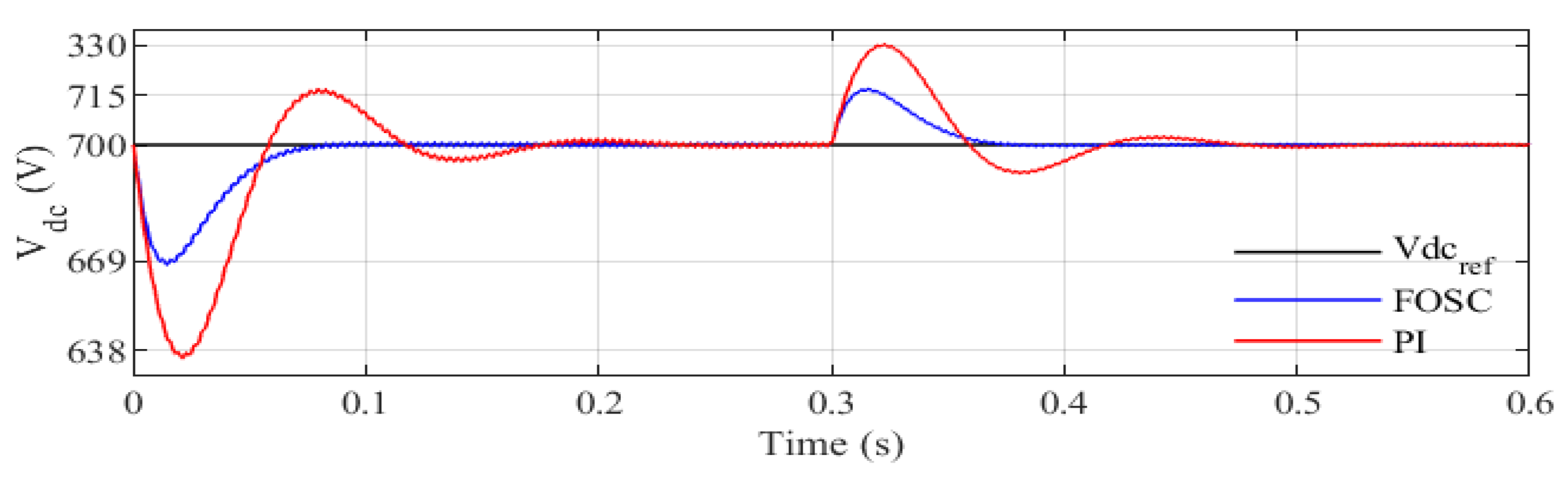
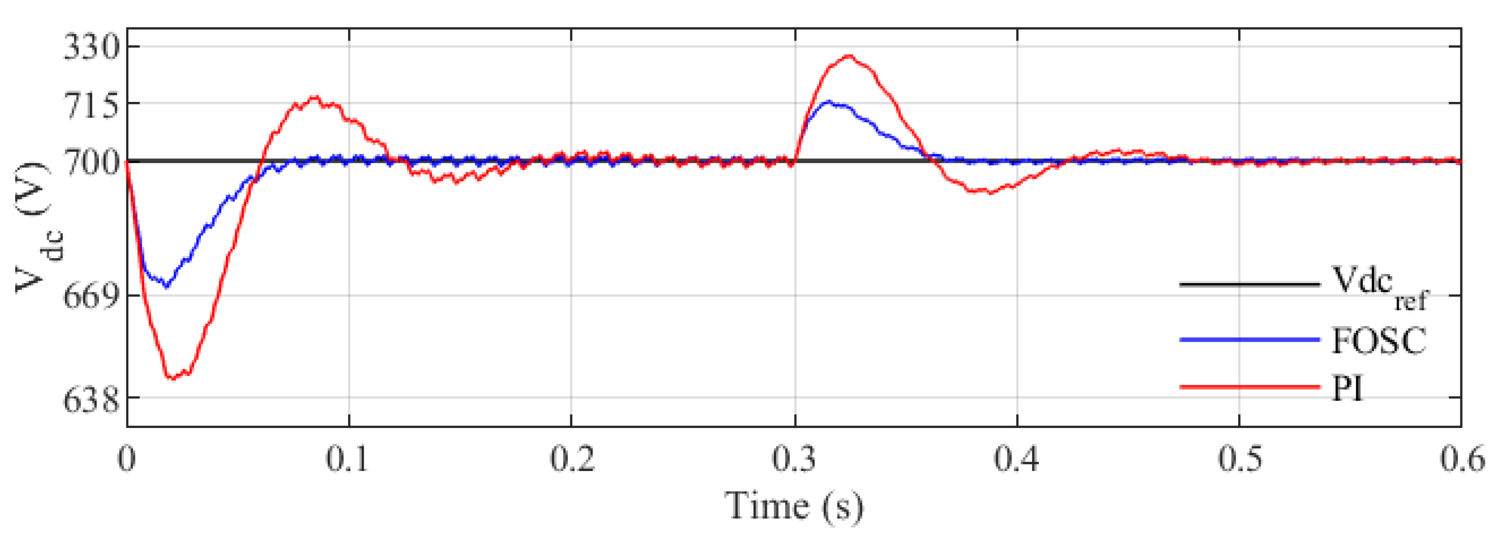
4.1. Design of a Dc-Link Voltage Controller
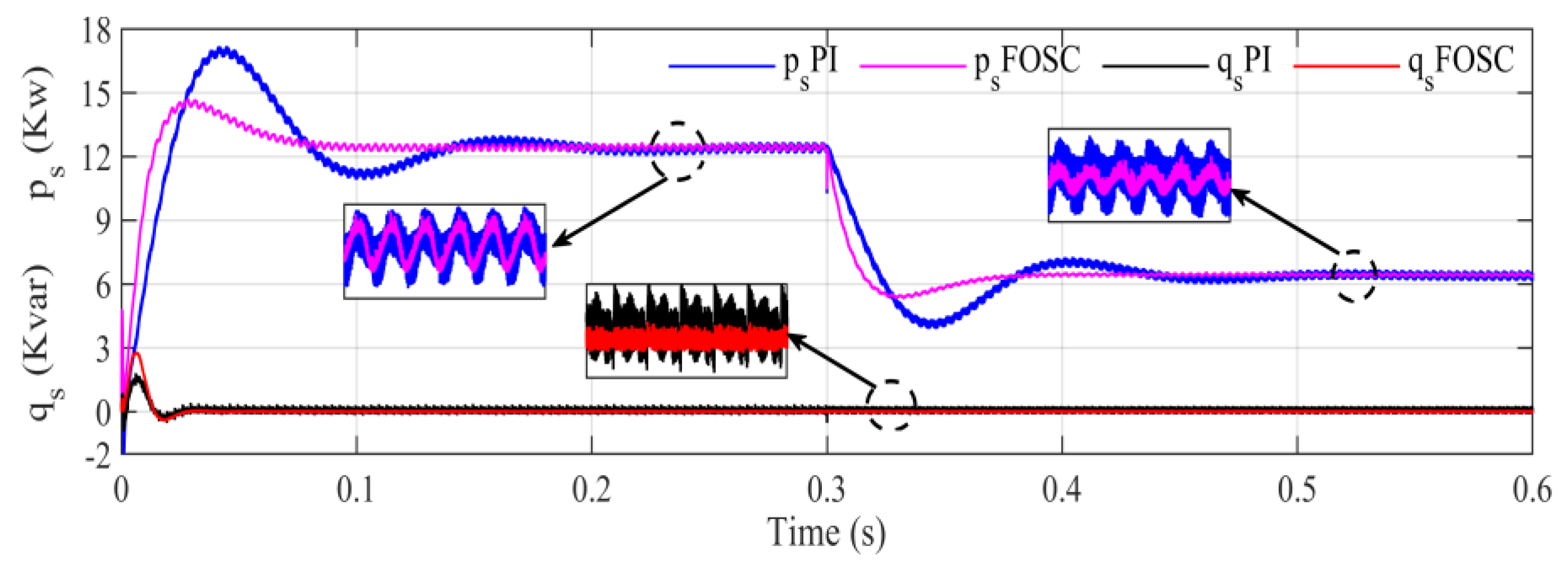
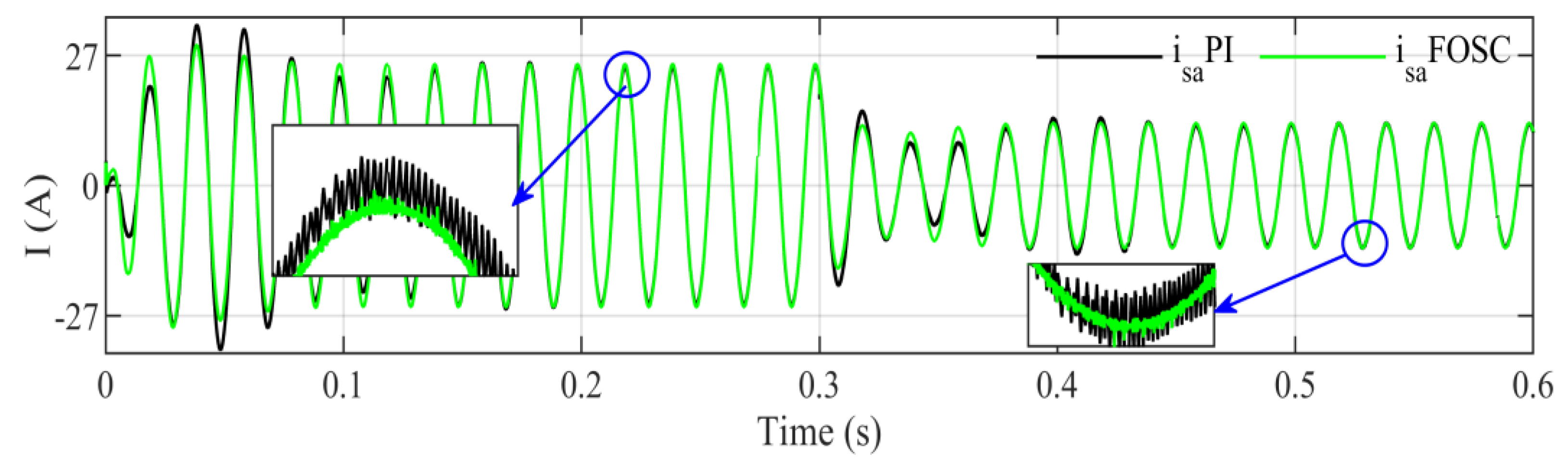
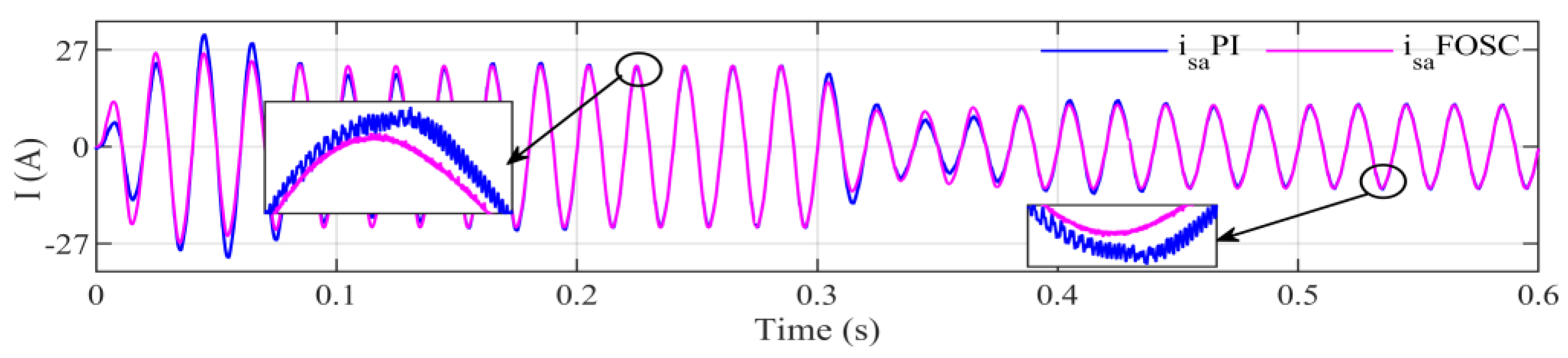
4.2. Design of Current Control
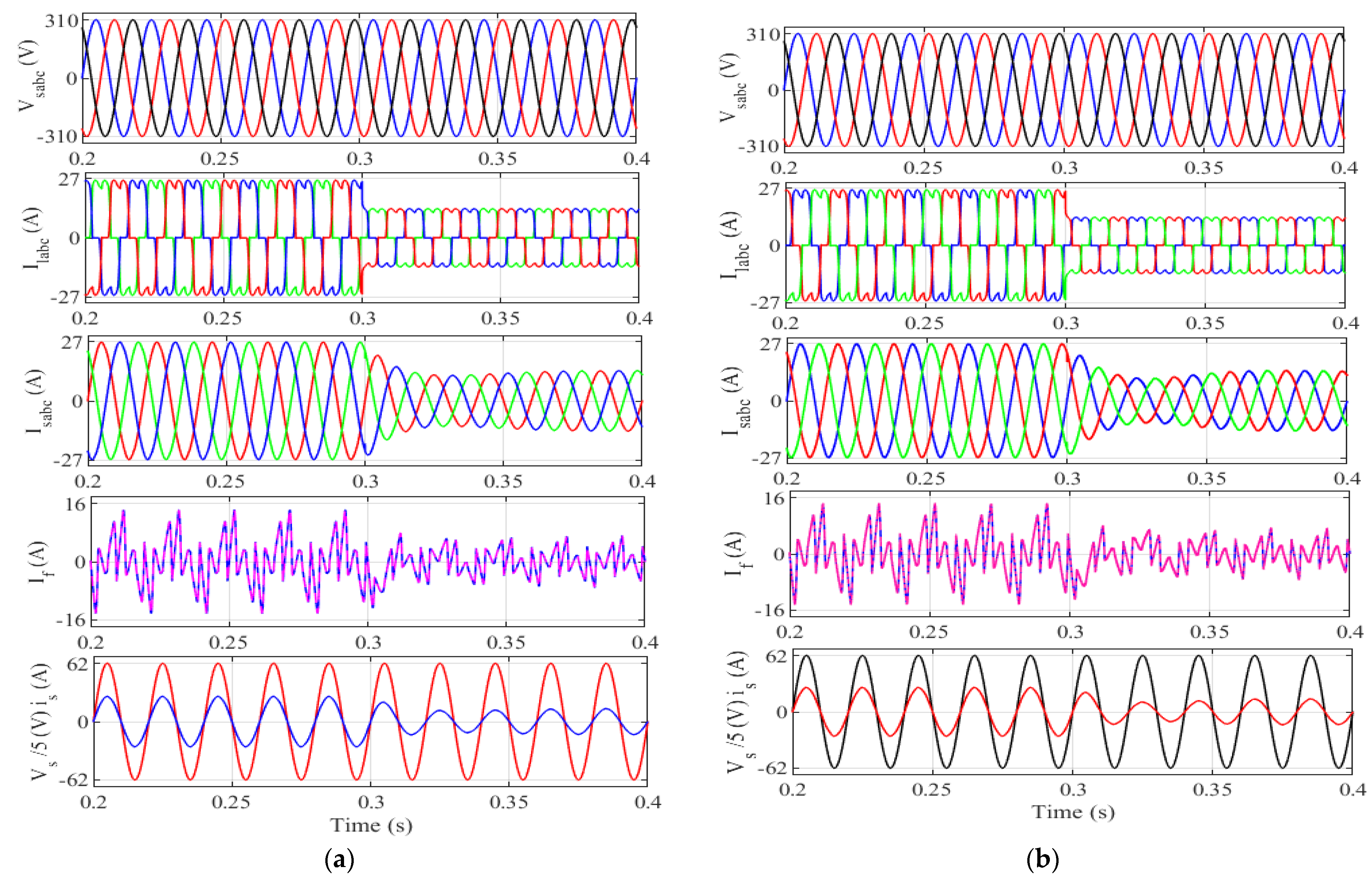
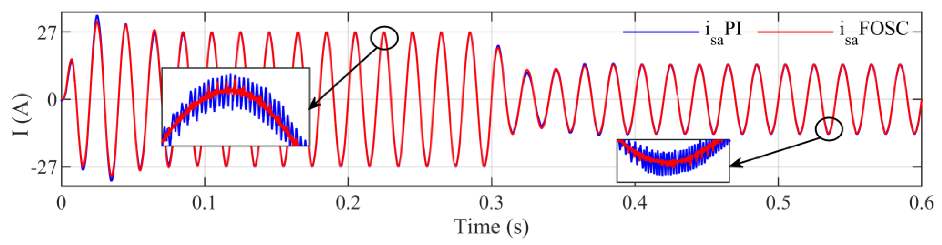
5. Results
- A.
- Source voltage balanced
- B.
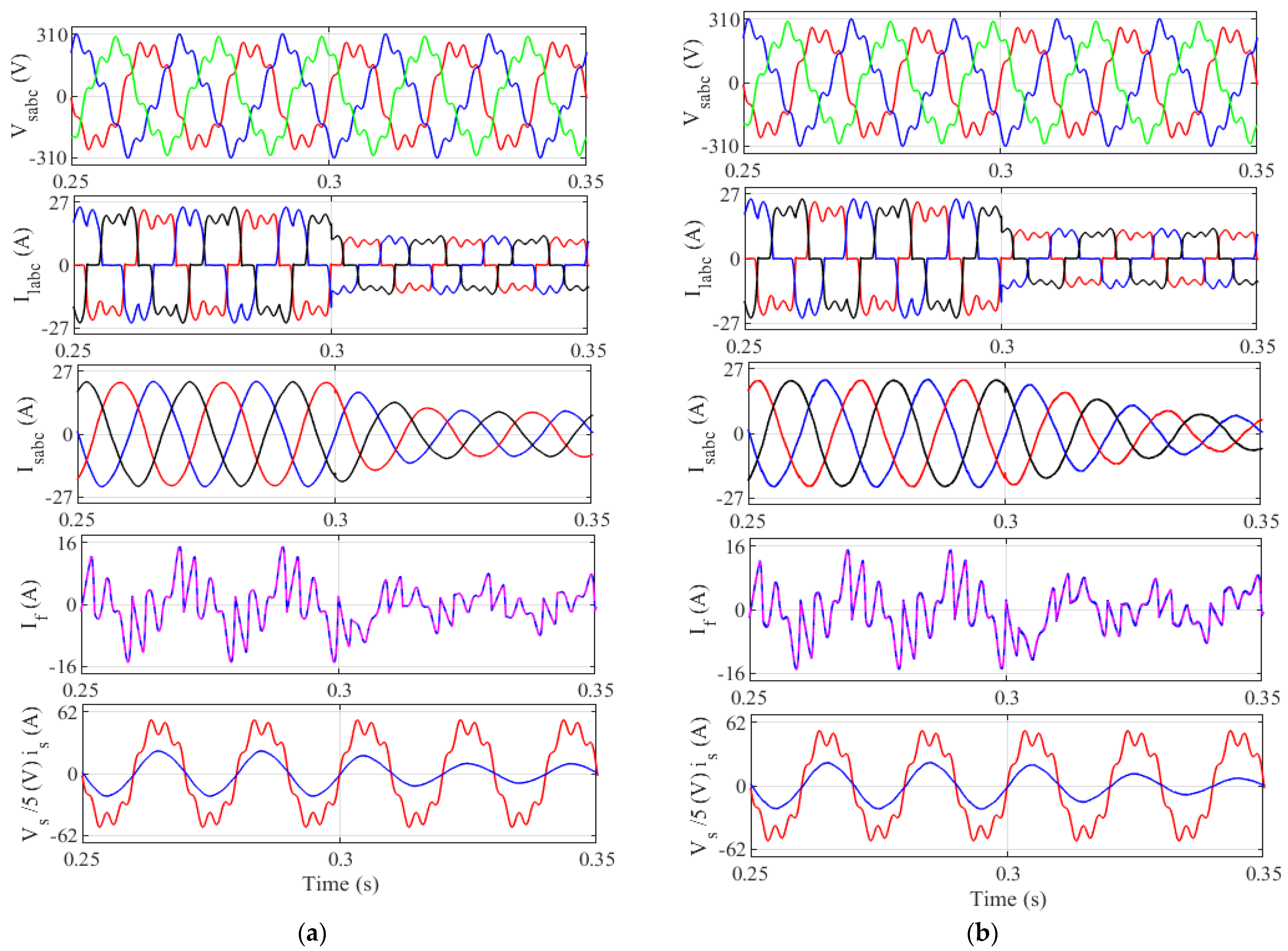
- Source voltage unbalanced
- C.
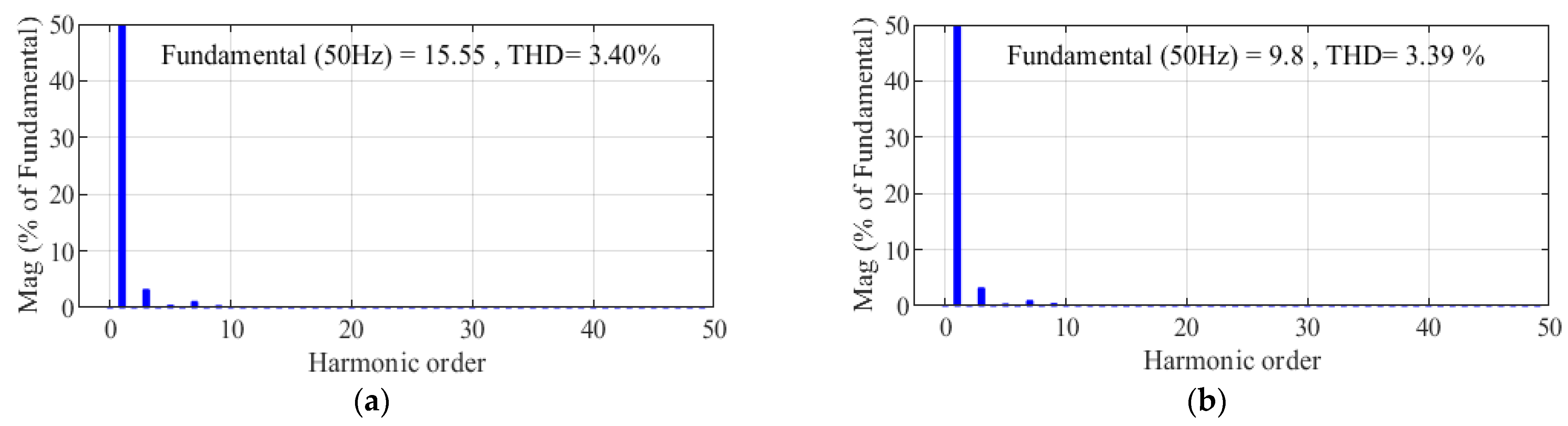
- Source voltage distorted
6. Conclusions
- -
- Improves the quality of the current and power;
- -
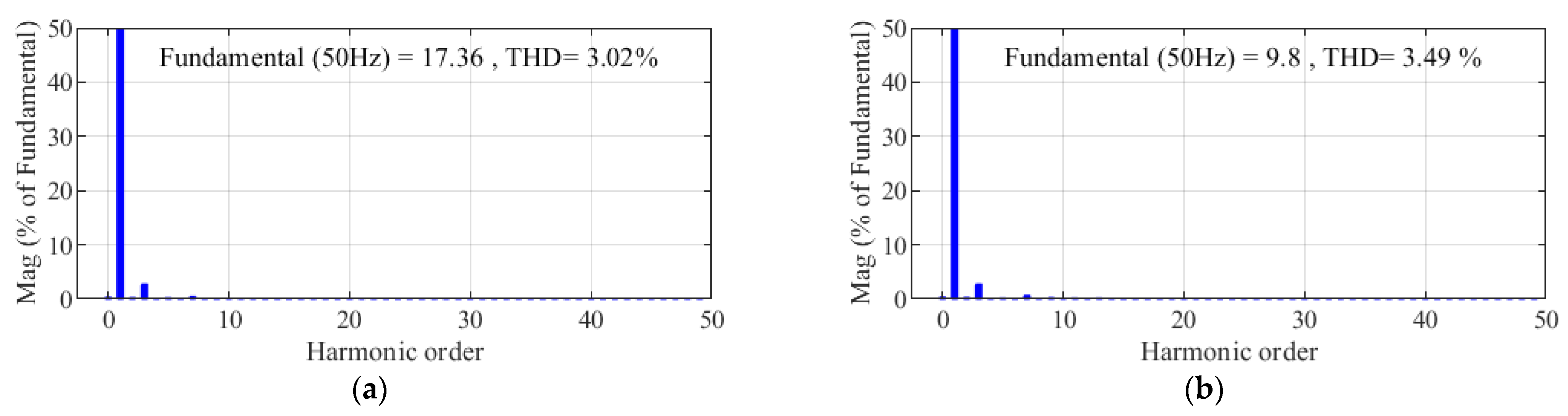
- Minimizes the THD value of the current;
- -
- Improvesthe settling time and reduces errors compared to traditional PI control.
Author Contributions
Funding
Data Availability Statement
Conflicts of Interest
Abbreviations
| PI | Proportional-integral |
| NPC | Neutral point clamped |
| FOSC | Fractional-order synergetic controller |
| PLL | Phase-locked loop |
| PWM | Pulse width modulation |
| STF | Self-tuning filter |
| SMC | Sliding mode control |
| SAPF | Shunt Active Power Filter |
| THD | Total harmonic distortion |
| DPC | Direct power control |
| SVM | Space vector modulation |
| VOC | Vector oriented control |
| PCC | Point of common coupling |
| MV | Macro-variable |
| BC | Backstepping controller |
| SC | Synergetic control |
| FOPI | Fractional-order proportional-integral |
References
- Michalec, Ł.; Jasiński, M.; Sikorski, T.; Leonowicz, Z.; Jasiński, Ł.; Suresh, V. Impact of Harmonic Currents of Nonlinear Loads on Power Quality of a Low Voltage Network—Review and Case Study. Energies 2021, 14, 3665. [Google Scholar] [CrossRef]
- Soliman, H.M.; Saleem, A.; Bayoumi, E.H.E.; De Santis, M. Harmonic Distortion Reduction of Transformer-Less Grid-Connected Converters by Ellipsoidal-Based Robust Control. Energies 2023, 16, 1362. [Google Scholar] [CrossRef]
- Karakaya, O.; Balci, M.E.; Hocaoglu, M.H. Minimization of Voltage Harmonic Distortion of Synchronous Generators under Non-Linear Loading via Modulated Field Current. Energies 2023, 16, 1789. [Google Scholar] [CrossRef]
- Sozanski, K.; Szczesniak, P. Advanced Control Algorithm for Three-Phase Shunt Active Power Filter Using Sliding DFT. Energies 2023, 16, 1453. [Google Scholar] [CrossRef]
- Park, B.; Lee, J.; Yoo, H.; Jang, G. Harmonic Mitigation Using Passive Harmonic Filters: Case Study in a Steel Mill Power System. Energies 2021, 14, 2278. [Google Scholar] [CrossRef]
- Massavie, V.; Despesse, G.; Carcouet, S.; Maynard, X. Comparison between Piezoelectric Filter and Passive LC Filter in a Class L−Piezo Inverter. Electronics 2022, 11, 3983. [Google Scholar] [CrossRef]
- Tan, K.-H.; Lin, F.-J.; Chen, J.-H. A Three-Phase Four-Leg Inverter-Based Active Power Filter for Unbalanced Current Compensation Using a Petri Probabilistic Fuzzy Neural Network. Energies 2017, 10, 2005. [Google Scholar] [CrossRef]
- Cao, X.; Dong, K.; Wei, X. An Improved Control Method Based on Source Current Sampled for Shunt Active Power Filters. Energies 2020, 13, 1405. [Google Scholar] [CrossRef]
- Habib, B.; Bizon, N. Advanced Direct Vector Control Method for Optimizing the Operation of a Double-Powered Induction Generator-Based Dual-Rotor Wind Turbine System. Mathematics 2021, 9, 2403. [Google Scholar] [CrossRef]
- Liu, J.; Hu, H.; Yu, S.S.; Trinh, H. Virtual Power Plant with Renewable Energy Sources and Energy Storage Systems for Sustainable Power Grid-Formation, Control Techniques and Demand Response. Energies 2023, 16, 3705. [Google Scholar] [CrossRef]
- Mahmoud, M.M.; Atia, B.S.; Esmail, Y.M.; Ardjoun, S.A.E.M.; Anwer, N.; Omar, A.I.; Alsaif, F.; Alsulamy, S.; Mohamed, S.A. Application of Whale Optimization Algorithm Based FOPI Controllers for STATCOM and UPQC to Mitigate Harmonics and Voltage Instability in Modern Distribution Power Grids. Axioms 2023, 12, 420. [Google Scholar] [CrossRef]
- Moschopoulos, G.; Jain, P. Single-phase single-stage power-factor-corrected converter topologies. IEEE Trans. Ind. Electron. 2005, 52, 23–35. [Google Scholar] [CrossRef]
- Ertl, H.; Kolar, J.W. A constant output current three-phase diode bridge rectifier employing a novel Electronic Smoothing Inductor. IEEE Trans. Ind. Electron. 2005, 52, 454–461. [Google Scholar] [CrossRef]
- Kiran Kumar, G.; Parimalasundar, E.; Elangovan, D.; Sanjeevikumar, P.; Lannuzzo, F.; Holm-Nielsen, J.B. Fault Investigation in Cascaded H-Bridge Multilevel Inverter through Fast Fourier Transform and Artificial Neural Network Approach. Energies 2020, 13, 1299. [Google Scholar] [CrossRef]
- Qanbari, T.; Tousi, B. Single-source three-phase multilevel inverter assembled by three-phase two-level inverter and two single-phase cascaded H-bridge inverters. IEEE Trans. Power Electron. 2020, 36, 5204–5212. [Google Scholar] [CrossRef]
- Chao, K.-H.; Ke, C.-H. Fault Diagnosis and Tolerant Control of Three-Level Neutral-Point Clamped Inverters in Motor Drives. Energies 2020, 13, 6302. [Google Scholar] [CrossRef]
- Mullali Kunnontakath Puthiyapurayil, M.R.; Nadir Nasirudeen, M.; Saywan, Y.A.; Ahmad, M.W.; Malik, H. A Review of Open-Circuit Switch Fault Diagnostic Methods for Neutral Point Clamped Inverter. Electronics 2022, 11, 3169. [Google Scholar] [CrossRef]
- Hoon, Y.; Mohd Radzi, M.A.; Hassan, M.K.; Mailah, N.F. A Dual-Function Instantaneous Power Theory for Operation of Three-Level Neutral-Point-Clamped Inverter-Based Shunt Active Power Filter. Energies 2018, 11, 1592. [Google Scholar] [CrossRef]
- Lee, J.S.; Kwak, R.; Lee, K.B. Novel discontinuous PWM method for a single-phase three-level neutral point clamped inverter with efficiency improvement and harmonic reduction. IEEE Trans. Power Electron. 2018, 33, 9253–9266. [Google Scholar] [CrossRef]
- Alnamer, S.S.; Mekhilef, S.; Mokhlis, H.; Tan, N. A Novel Multilevel DC-Link Three-Phase T-Type Inverter. Energies 2020, 13, 4186. [Google Scholar] [CrossRef]
- Buła, D.; Jarek, G.; Michalak, J.; Zygmanowski, M. Control Method of Four Wire Active Power Filter Based on Three-Phase Neutral Point Clamped T-Type Converter. Energies 2021, 14, 8427. [Google Scholar] [CrossRef]
- Long, B.; Cao, T.; Qi, X.; Shen, D.; Guerrero, J.M.; Rodriguez, J.; Chong, K.T. Noninteger Lexicographic-Optimization-Based Sequential Model-Predictive Fault-Tolerant Control of T-Type Shunt Active Power Filter. IEEE Trans. Power Electron. 2021, 37, 7169–7184. [Google Scholar] [CrossRef]
- Escobar, G.; Martinez-Rodriguez, P.R.; Iturriaga-Medina, S.; Vazquez-Guzman, G.; Sosa-Zuñiga, J.M.; Langarica-Cordoba, D. Control Design and Experimental Validation of a HB-NPC as a Shunt Active Power Filter. Energies 2020, 13, 1691. [Google Scholar] [CrossRef]
- Chen, C.-I.; Lan, C.-K.; Chen, Y.-C.; Chen, C.-H. Adaptive Frequency-Based Reference Compensation Current Control Strategy of Shunt Active Power Filter for Unbalanced Nonlinear Loads. Energies 2019, 12, 3080. [Google Scholar] [CrossRef]
- Madasamy, P.; Suresh Kumar, V.; Sanjeevikumar, P.; Holm-Nielsen, J.B.; Hosain, E.; Bharatiraja, C. A Three-Phase Transformerless T-Type- NPC-MLI for Grid Connected PV Systems with Common-Mode Leakage Current Mitigation. Energies 2019, 12, 2434. [Google Scholar] [CrossRef]
- Xie, L.; Yao, J. Common-Mode Voltage Reduction and Neutral Point Voltage Balance Modulation Technology of Quasi-Z-Source T-Type Three-Level Inverter. Electronics 2022, 11, 2203. [Google Scholar] [CrossRef]
- Habib, B.; Boudjema, Z.; Belaidi, A. DFIG-based wind turbine system using three-level neural space vector modulation technique. Majlesi J. Mechatron. Syst. 2018, 7, 35–45. [Google Scholar]
- Habib, B. Sliding mode with neural network regulateur for DFIG using two-level NPWM strategy. Iran. J. Electr. Electron. Eng. 2019, 15, 411–419. [Google Scholar]
- Habib, B.; Boudjema, Z.; Belaidi, A. Using three-level Fuzzy space vector modulation method to improve indirect vector control strategy of a DFIG based wind energy conversion systems. Int. J. Smart Grid 2018, 2, 155–171. [Google Scholar]
- Habib, B.; Bizon, N.; Colak, I. A Brief Review of Space Vector Modulation (SVM) Methods and a New SVM Technique Based on the Minimum and Maximum of the Three-Phase Voltages. Iran. J. Electr. Electron. Eng. 2022, 18, 1–18. [Google Scholar] [CrossRef]
- Cittanti, D.; Gregorio, M.; Bossotto, E.; Mandrile, F.; Bojoi, R. Full Digital Control and Multi-Loop Tuning of a Three-Level T-Type Rectifier for Electric Vehicle Ultra-Fast Battery Chargers. Electronics 2021, 10, 1453. [Google Scholar] [CrossRef]
- Benbouhenni, H.; Boudjema, Z.; Bizon, N.; Thounthong, P.; Takorabet, N. Direct Power Control Based on Modified Sliding Mode Controller for a Variable-Speed Multi-Rotor Wind Turbine System Using PWM Strategy. Energies 2022, 15, 3689. [Google Scholar] [CrossRef]
- Gao, Y.; Li, X.; Zhang, W.; Hou, D.; Zheng, L. A Sliding Mode Control Strategy with Repetitive Sliding Surface for Shunt Active Power Filter with an LCLCL Filter. Energies 2020, 13, 1740. [Google Scholar] [CrossRef]
- Toumi, T.; Allali, A.; Meftouhi, A.; Abdelkhalek, O.; Benabdelkader, A.; Denai, M. Robust control of series active power filters for power quality enhancement in distribution grids: Simulation and experimental validation. ISA Trans. 2020, 107, 350–359. [Google Scholar] [CrossRef]
- Silaa, M.Y.; Derbeli, M.; Barambones, O.; Cheknane, A. Design and Implementation of High Order Sliding Mode Control for PEMFC Power System. Energies 2020, 13, 4317. [Google Scholar] [CrossRef]
- Benbouhenni, H.; Bizon, N. Improved Rotor Flux and Torque Control Based on the Third-Order Sliding Mode Scheme Applied to the Asynchronous Generator for the Single-Rotor Wind Turbine. Mathematics 2021, 9, 2297. [Google Scholar] [CrossRef]
- Benbouhenni, H.; Bizon, N. Third-Order Sliding Mode Applied to the Direct Field-Oriented Control of the Asynchronous Generator for Variable-Speed Contra-Rotating Wind Turbine Generation Systems. Energies 2021, 14, 5877. [Google Scholar] [CrossRef]
- Ali, M.N.; Mahmoud, K.; Lehtonen, M.; Darwish, M.M.F. Promising MPPT Methods Combining Metaheuristic, Fuzzy-Logic and ANN Techniques for Grid-Connected Photovoltaic. Sensors 2021, 21, 1244. [Google Scholar] [CrossRef]
- Musa, S.; Radzi, M.A.M.; Hizam, H.; Wahab, N.I.A.; Hoon, Y.; Zainuri, M.A.A.M. Modified Synchronous Reference Frame Based Shunt Active Power Filter with Fuzzy Logic Control Pulse Width Modulation Inverter. Energies 2017, 10, 758. [Google Scholar] [CrossRef]
- Benbouhenni, H.; Bizon, N.; Colak, I.; Thounthong, P.; Takorabet, N. Application of Fractional-Order PI Controllers and Neuro-Fuzzy PWM Technique to Multi-Rotor Wind Turbine Systems. Electronics 2022, 11, 1340. [Google Scholar] [CrossRef]
- Habib, B.; Bizon, N. A Synergetic Sliding Mode Controller Applied to Direct Field-Oriented Control of Induction Generator-Based Variable Speed Dual-Rotor Wind Turbines. Energies 2021, 14, 4437. [Google Scholar] [CrossRef]
- Habib, B.; Bizon, N. Terminal Synergetic Control for Direct Active and Reactive Powers in Asynchronous Generator-Based Dual-Rotor Wind Power Systems. Electronics 2021, 10, 1880. [Google Scholar] [CrossRef]
- Ali, A.I.M.; Sayed, M.A.; Mohamed, A.A.S. Seven-Level Inverter with Reduced Switches for PV System Supporting Home-Grid and EV Charger. Energies 2021, 14, 2718. [Google Scholar] [CrossRef]
- Cano, J.M.; Martin, A.D.; Herrera, R.S.; Vazquez, J.R.; Ruiz-Rodriguez, F.J. Grid-Connected PV Systems Controlled by Sliding via Wireless Communication. Energies 2021, 14, 1931. [Google Scholar] [CrossRef]
- Khalkhali, H.; Oshnoei, A.; Anvari-Moghaddam, A. Proportional Hysteresis Band Control for DC Voltage Stability of Three-Phase Single-Stage PV Systems. Electronics 2022, 11, 452. [Google Scholar] [CrossRef]
- Abdusalam, M.; Poure, P.; Karimi, S.; Saadate, S. New digital reference current generation for shunt active power filter under distorted voltage conditions. Electr. Power Syst. Res. 2009, 79, 759–765. [Google Scholar] [CrossRef]
- Chedjara, Z.; Massoum, A.; Massoum, S.; Wira, P.; Safa, A.; Gouichiche, A. A novel robust PLL algorithm applied to the control of a shunt active power filter using a self-tuning filter concept. In Proceedings of the 2018 IEEE International Conference on Industrial Technology (ICIT), Lyon, France, 20–22 February 2018. [Google Scholar] [CrossRef]
- Hoon, Y.; Mohd Radzi, M.A.; Hassan, M.K.; Mailah, N.F. A Refined Self-Tuning Filter-Based Instantaneous Power Theory Algorithm for Indirect Current Controlled Three-Level Inverter-Based Shunt Active Power Filters under Non-sinusoidal Source Voltage Conditions. Energies 2017, 10, 277. [Google Scholar] [CrossRef]
- Hoon, Y.; Mohd Radzi, M.A.; Hassan, M.K.; Mailah, N.F. A Self-Tuning Filter-Based Adaptive Linear Neuron Approach for Operation of Three-Level Inverter-Based Shunt Active Power Filters under Non-Ideal Source Voltage Conditions. Energies 2017, 10, 667. [Google Scholar] [CrossRef]
- Chao, K.-H.; Chang, L.-Y.; Hung, C.-C. Fault Diagnosis and Tolerant Control for Three-Level T-Type Inverters. Electronics 2022, 11, 2496. [Google Scholar] [CrossRef]
- Yin, Z.; Hu, C.; Luo, K.; Rui, T.; Feng, Z.; Lu, G.; Zhang, P. A Novel Model-Free Predictive Control for T-Type Three-Level Grid-Tied Inverters. Energies 2022, 15, 6557. [Google Scholar] [CrossRef]
- Ghanim, F.; Al-Janaby, H.F.; Bazighifan, O. Some New Extensions on Fractional Differential and Integral Properties for Mittag-Leffler Confluent Hypergeometric Function. Fractal Fract. 2021, 5, 143. [Google Scholar] [CrossRef]
- Ahmed, I.; Kumam, P.; Shah, K.; Borisut, P.; Sitthithakerngkiet, K.; Ahmed Demba, M. Stability Results for Implicit Fractional Pantograph Differential Equations via ϕ-Hilfer Fractional Derivative with a Nonlocal Riemann-Liouville Fractional Integral Condition. Mathematics 2020, 8, 94. [Google Scholar] [CrossRef]
- Luchko, Y. Fractional Differential Equations with the General Fractional Derivatives of Arbitrary Order in the Riemann–Liouville Sense. Mathematics 2022, 10, 849. [Google Scholar] [CrossRef]
- Farid, G.; Nazeer, W.; Saleem, M.S.; Mehmood, S.; Kang, S.M. Bounds of Riemann-Liouville Fractional Integrals in General Form via Convex Functions and Their Applications. Mathematics 2018, 6, 248. [Google Scholar] [CrossRef]
- Obukhova, E.; Veselov, G.E.; Obukhov, P.; Beskopylny, A.; Stel’makh, S.A.; Shcherban’, E.M. Synergetic Synthesis of Nonlinear Laws of Throttle Control of a Pneumatic Drive. Appl. Sci. 2022, 12, 1797. [Google Scholar] [CrossRef]
- Al-Hussein, A.-B.A.; Tahir, F.R.; Ouannas, A.; Sun, T.-C.; Jahanshahi, H.; Aly, A.A. Chaos Suppressing in a Three-Buses Power System Using an Adaptive Synergetic Control Method. Electronics 2021, 10, 1532. [Google Scholar] [CrossRef]
- Nicola, M.; Nicola, C.-I. Improved Performance in the Control of DC-DC Three-Phase Power Electronic Converter Using Fractional-Order SMC and Synergetic Controllers and RL-TD3 Agent. Fractal Fract. 2022, 6, 729. [Google Scholar] [CrossRef]
- Nicola, M.; Nicola, C.-I. Fractional-Order Control of Grid-Connected Photovoltaic System Based on Synergetic and Sliding Mode Controllers. Energies 2021, 14, 510. [Google Scholar] [CrossRef]
- Agarwal, R.; Hristova, S.; O’Regan, D. Stability of Generalized Proportional Caputo Fractional Differential Equations by Lyapunov Functions. Fractal Fract. 2022, 6, 34. [Google Scholar] [CrossRef]
- Farag, M.M.; Patel, N.; Hamid, A.K.; Adam, A.A.; Bansal, R.C.; Bettayeb, M.; Mehiri, A. An Optimized Fractional Nonlinear Synergic Controller for Maximum Power Point Tracking of Photovoltaic Array under Abrupt Irradiance Change. IEEE J. Photovolt. 2023, 13, 305–314. [Google Scholar] [CrossRef]
- Zhang, S.; Kang, J.; Yuan, J. An optimized overmodulation synchronized SVPWM scheme for three-level NPC inverters with low switching frequency. CSEE J. Power Energy Syst. 2022, 14, 1–14. [Google Scholar]
- Ayachi Amor, Y.; Hamoudi, F.; Kheldoun, A.; Didier, G.; Rabiai, Z. Fuzzy logic enhanced control for a single-stage grid-tied photovoltaic system with shunt active filtering capability. Int. Trans. Electr. Energy Syst. 2021, 10, e13008. [Google Scholar] [CrossRef]
- Kovačević, H.; Korošec, L.; Milanovič, M. Single-Shunt Three-Phase Current Measurement for a Three-Level Inverter Using a Modified Space-Vector Modulation. Electronics 2021, 10, 1734. [Google Scholar] [CrossRef]
- Do, D.-T.; Nguyen, M.-K.; Ngo, V.-T.; Quach, T.-H.; Tran, V.-T. Common Mode Voltage Elimination for Quasi-Switch Boost T-Type Inverter Based on SVM Technique. Electronics 2020, 9, 76. [Google Scholar] [CrossRef]
- Madasamy, P.; Pongiannan, R.K.; Ravichandran, S.; Padmanaban, S.; Chokkalingam, B.; Hossain, E.; Adedayo, Y. A Simple Multilevel Space Vector Modulation Technique and MATLAB System Generator Built FPGA Implementation for Three-Level Neutral-Point Clamped Inverter. Energies 2019, 12, 4332. [Google Scholar] [CrossRef]
- Bekhoucha, N.; Mesbahi, N.; Bouchikha, H.; Heguig, L.; Chikha, S. Model Predictive Control of Three-Level Shunt Active Power Filter Connected to a Photovoltaic System. In Proceedings of the 2022 19th International Multi-Conference on Systems, Signals & Devices (SSD), Sétif, Algeria, 6–10 May 2022; pp. 128–133. [Google Scholar] [CrossRef]


| States | Status of Switching Devices (x = 1, 2, 3) (1 = ON, 0 = OFF) | Voltage | |||
|---|---|---|---|---|---|
| Tx1 | Tx2 | Tx3 | Tx4 | ||
| P | 1 | 1 | 0 | 0 | Vdc/2 |
| O | 0 | 1 | 1 | 0 | 0 |
| N | 0 | 0 | 1 | 1 | Vdc/2 |
| Parameter | Value |
|---|---|
| Source voltage and frequency | 220 V, 50 Hz |
| 5 mΩ, 3 mH | |
| 0.1 Ω, 3 mH | |
| 40 Ω, 10 mH | |
| 1.2 mΩ, 0.2 mH | |
| 4 mF | |
| Total DC-bus voltage reference | 700 V |
| Transient Time (s) | Settling Time (s) | Overshoot/Undershoot (%) | ||
|---|---|---|---|---|
| FOSC | PI | FOSC | PI | |
| 0 | 0.08 | 0.22 | 4.4 | 8.85 |
| 0.3 | 0.07 | 0.18 | 2.14 | 4.28 |
| Source Voltages and Currents | Phases | FOSC | PI | ||||
|---|---|---|---|---|---|---|---|
| t < 0.3 s | t > 0.3 s | t < 0.3 s | t > 0.3 s | ||||
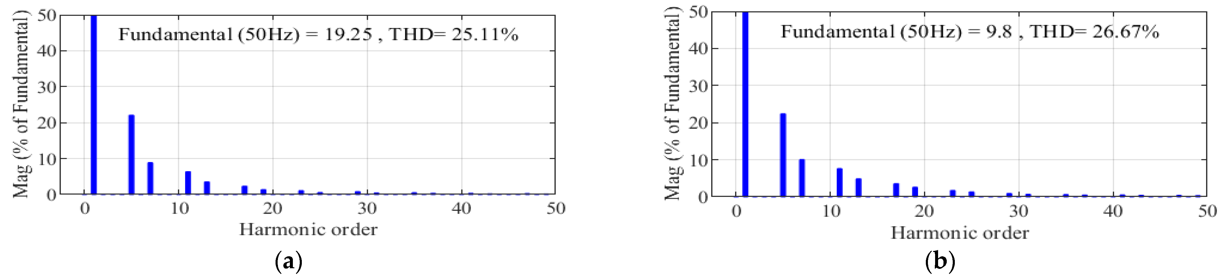
| Source current before filtering | THD (%) | Ph-1 | 25.11 | 26.67 | 25.11 | 26.67 | |
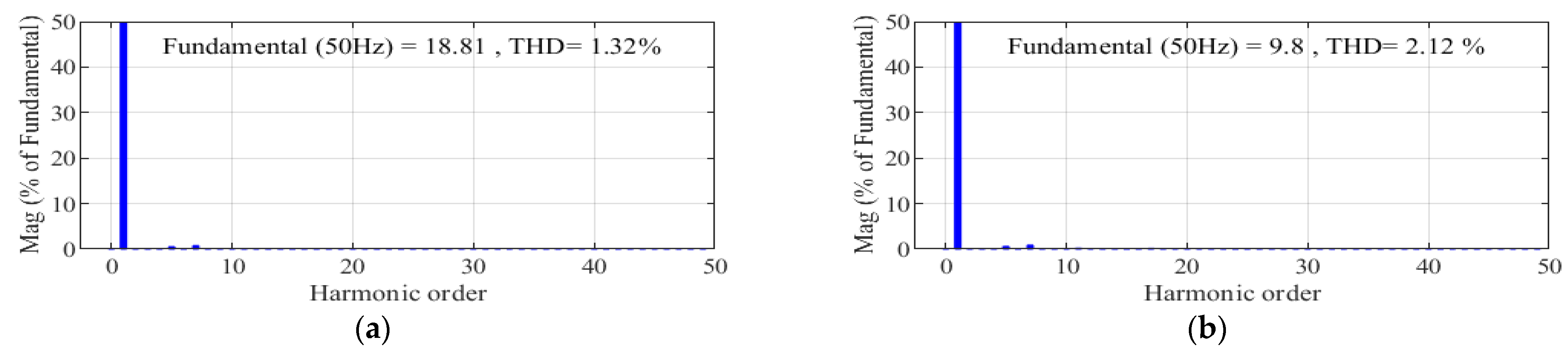
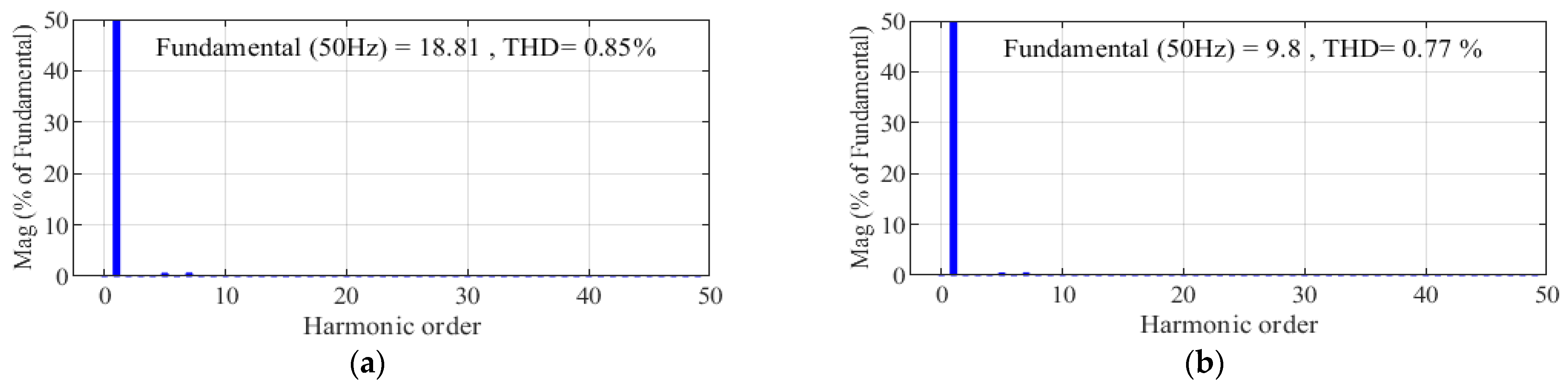
| Source voltages | Balanced | THD (%) | Ph-1 | 0.85 | 0.77 | 1.32 | 2.12 |
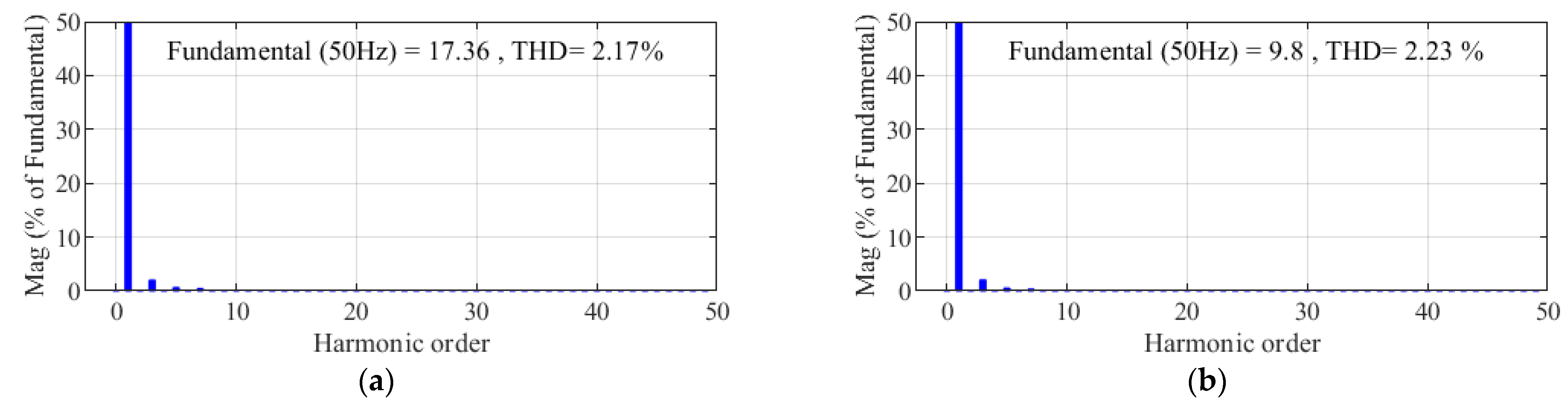
| Unbalanced | THD (%) | Ph-1 | 2.17 | 2.23 | 3.02 | 3.49 | |
| Ph-2 | 2.27 | 2.33 | 2.90 | 3.31 | |||
| Ph-3 | 1.78 | 1.93 | 2.70 | 3.42 | |||
| Distorted | THD (%) | Ph-1 | 3.40 | 3.39 | 3.51 | 4.11 | |
| Ph-2 | 3.44 | 3.49 | 3.41 | 4.17 | |||
| Ph-3 | 2.90 | 3.04 | 3.23 | 4.25 | |||
Disclaimer/Publisher’s Note: The statements, opinions and data contained in all publications are solely those of the individual author(s) and contributor(s) and not of MDPI and/or the editor(s). MDPI and/or the editor(s) disclaim responsibility for any injury to people or property resulting from any ideas, methods, instructions or products referred to in the content. |
© 2023 by the authors. Licensee MDPI, Basel, Switzerland. This article is an open access article distributed under the terms and conditions of the Creative Commons Attribution (CC BY) license (https://creativecommons.org/licenses/by/4.0/).
Share and Cite
Deffaf, B.; Debdouche, N.; Benbouhenni, H.; Hamoudi, F.; Bizon, N. A New Control for Improving the Power Quality Generated by a Three-Level T-Type Inverter. Electronics 2023, 12, 2117. https://doi.org/10.3390/electronics12092117
Deffaf B, Debdouche N, Benbouhenni H, Hamoudi F, Bizon N. A New Control for Improving the Power Quality Generated by a Three-Level T-Type Inverter. Electronics. 2023; 12(9):2117. https://doi.org/10.3390/electronics12092117
Chicago/Turabian StyleDeffaf, Brahim, Naamane Debdouche, Habib Benbouhenni, Farid Hamoudi, and Nicu Bizon. 2023. "A New Control for Improving the Power Quality Generated by a Three-Level T-Type Inverter" Electronics 12, no. 9: 2117. https://doi.org/10.3390/electronics12092117
APA StyleDeffaf, B., Debdouche, N., Benbouhenni, H., Hamoudi, F., & Bizon, N. (2023). A New Control for Improving the Power Quality Generated by a Three-Level T-Type Inverter. Electronics, 12(9), 2117. https://doi.org/10.3390/electronics12092117