
A CSAR 3D Imaging Method Suitable for Edge Computation


Abstract
:1. Introduction
2. BP 3D Imaging
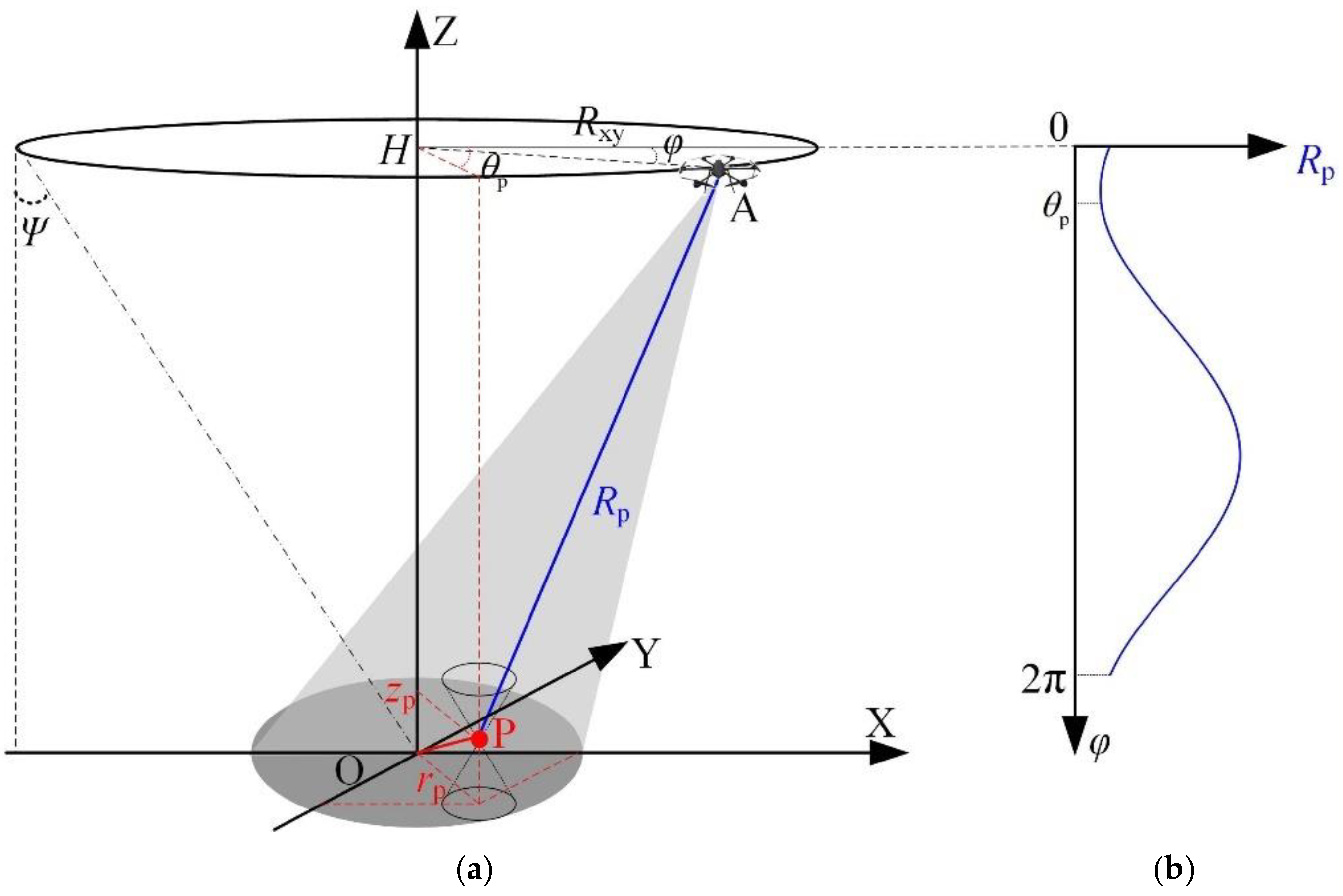
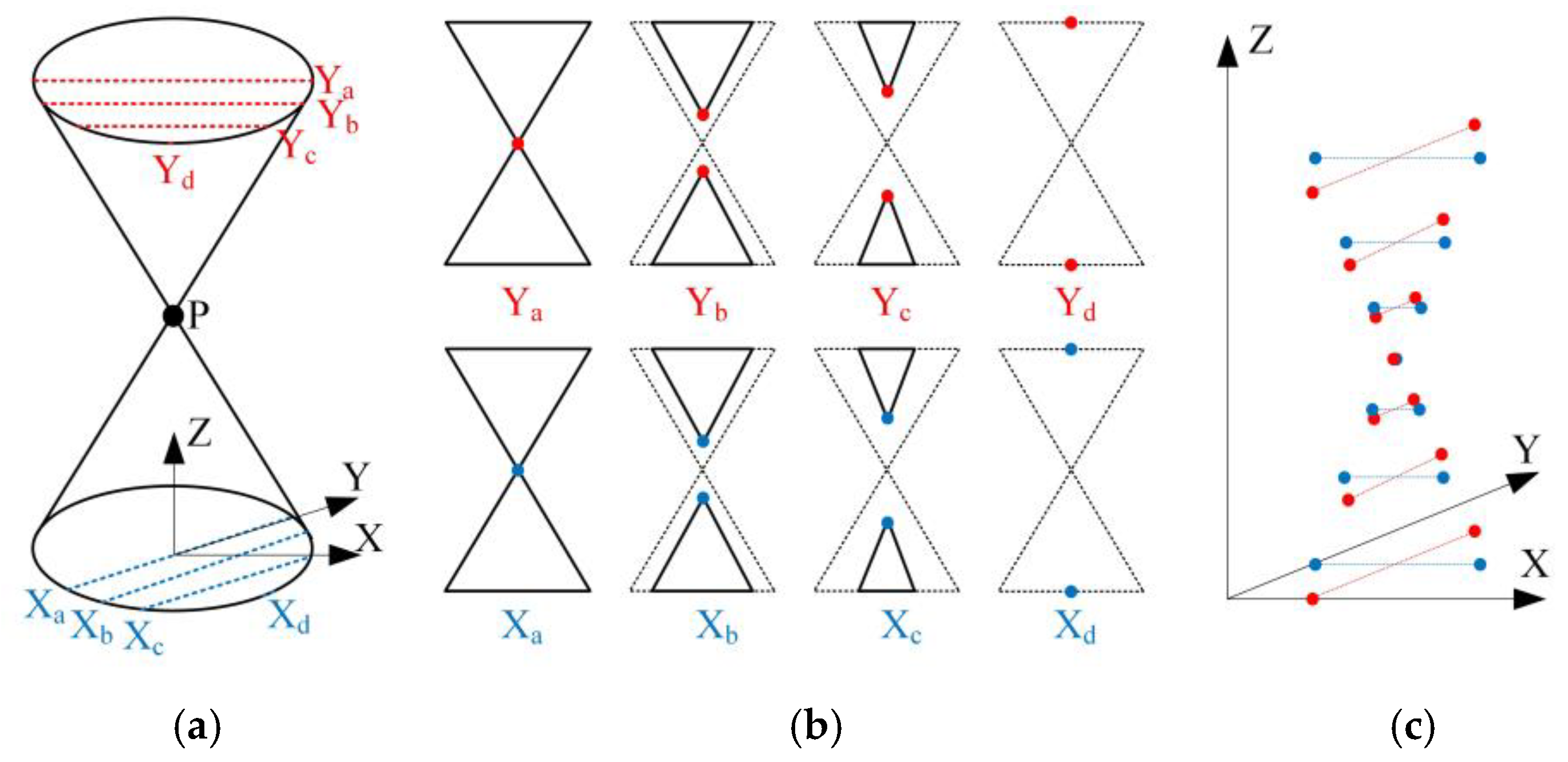
2.1. Imaging Geometric Model of CSAR
2.2. BP 3D Imaging
2.2.1. Traditional BP 3D Imaging
2.2.2. IBP 3D Imaging
3. A CSAR 3D Imaging Method Suitable for Edge Computation
3.1. Principle of the Method
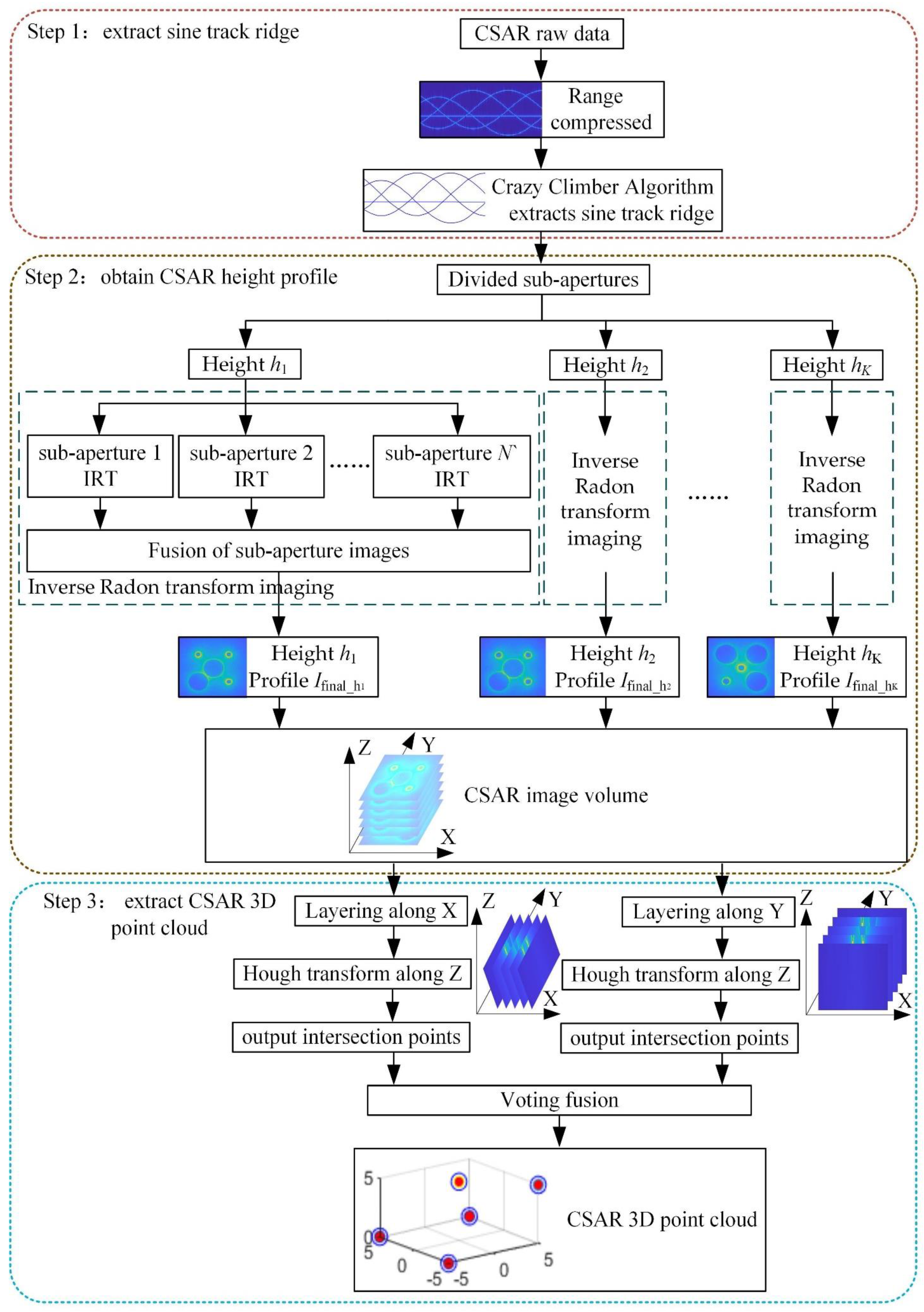
3.2. Algorithm Flow
3.3. Algorithm Complexity Analysis
4. Data Processing
4.1. Simulation Data Processing
 ” in Figure 9b; and the intersection point of the detected output line is shown as the cyan “
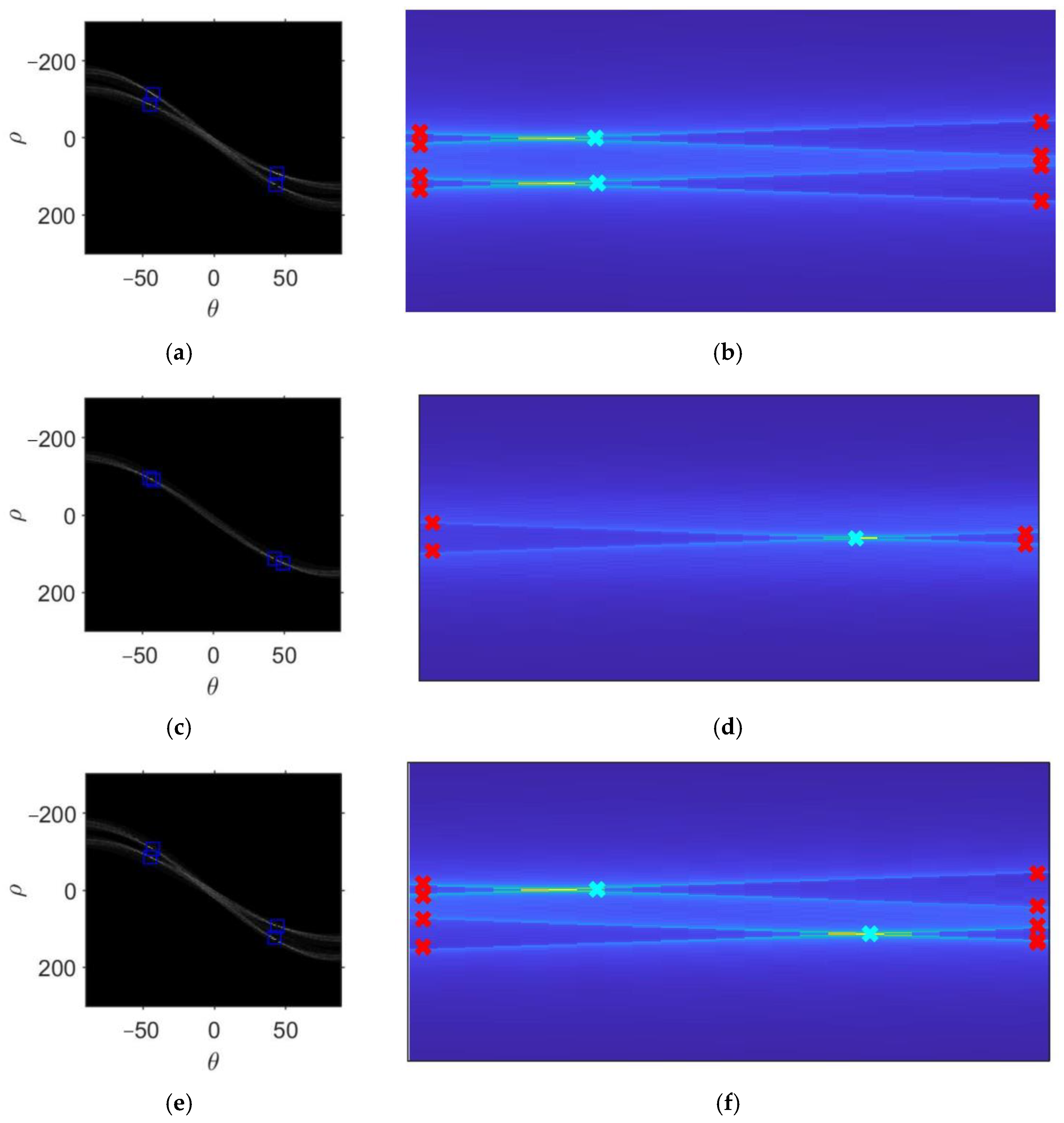
 ” in Figure 9b. Here, the two intersection points are consistent with the two-point target with a height of z = 0 m in the scene. When x = 0 m, the peak point after the Hough transform is extracted, as shown in Figure 9c, and the intersection point of the extracted straight line and the detected output straight line is shown in Figure 9d. When x = 5 m, the peak point after the Hough transform is extracted, as shown in Figure 9e, and the intersection point of the extracted straight line and the detected output straight line is shown in Figure 9f. The two intersection points are located at different heights, consistent with heights of z = 0 m and z = 5 m in the scene.
4.2. Measured Data Processing
5. Conclusions
Author Contributions
Funding
Institutional Review Board Statement
Informed Consent Statement
Data Availability Statement
Conflicts of Interest
Abbreviations
| CSAR | Circular synthetic aperture radar |
| 2D | Two-dimensional |
| 3D | Three-dimensional |
| BP | Back projection |
| FMCW | Frequency-modulated continuous wave |
| GLRT | Generalized likelihood ratio test |
| IBP | Improved BP |
| IRT | Inverse Radon transform |
| IoT | Internet of Things |
| SRUAV | Small rotor unmanned aerial vehicle |
References
- Hu, X.; Liu, Z.; Yu, X.; Zhao, Y.; Chen, W.; Hu, B.; Du, X.; Li, X.; Helaoui, M. Convolutional Neural Network for Behavioral Modeling and Predistortion of Wideband Power Amplifiers. IEEE Trans. Neural Netw. Learn. Syst. 2022, 33, 3923–3937. [Google Scholar] [CrossRef] [PubMed]
- Hu, X.; Zhang, Y.; Liao, X.; Liu, Z.; Wang, W.; Ghannouchi, F.M. Dynamic Beam Hopping Method Based on Multi-Objective Deep Reinforcement Learning for Next Generation Satellite Broadband Systems. IEEE Trans. Broadcast. 2020, 66, 630–646. [Google Scholar] [CrossRef]
- Zuo, F.; Li, J.; Hu, R.; Pi, Y. Unified coordinate system algorithm for terahertz video-SAR image formation. IEEE Trans. Terahertz Sci. Technol. 2018, 8, 725–735. [Google Scholar] [CrossRef]
- Han, D.; Zhou, L.; Jiao, Z.; Wu, Y. A coherent 3-D imaging method for multi-circular SAR based on an improved 3-D back projection algorithm. J. Electron. Inf. Technol. 2021, 43, 131–137. [Google Scholar]
- Li, Y.; Chen, L.; An, D.; Zhou, Z. A novel DEM extraction method based on chain correlation of CSAR subaperture images. IEEE J. Sel. Top. Appl. Earth Obs. Remote Sens. 2021, 14, 8718–8728. [Google Scholar] [CrossRef]
- Zhang, J.; Suo, Z.; Li, Z.; Bao, Z. Joint cross-correlation DEM extraction method for CSAR subaperture image sequences. Syst. Eng. Electron. 2018, 40, 1939–1944. [Google Scholar]
- Feng, S.; Lin, Y.; Wang, Y.; Teng, F.; Hong, W. 3D Point Cloud Reconstruction Using Inversely Mapping and Voting from Single Pass CSAR Images. Remote Sens. 2021, 13, 3534. [Google Scholar] [CrossRef]
- Zhang, X.; Shi, J.; Wei, S. Three Dimensional Synthetic Aperture Radar; National Defense Industry Press: Beijing, China, 2017. [Google Scholar]
- Bao, Z.; Xing, M.; Wang, T. Radar Imaging Technique; Electronic Industry Press: Beijing, China, 2005. [Google Scholar]
- Ma, Y.; Chu, L.; Yang, X.; Hou, X. SAR autofocusing method based on slant range wavenumber subband division. J. Eng. Univ. PLA 2022, 1, 12–21. [Google Scholar]
- Kan, X.; Li, Y.; Wang, H.; Wang, Y.; Fu, C. A new algorithm of fast back projection in circular SAR. Guid. Fuze 2018, 39, 10–14. [Google Scholar]
- Stankovic, L.; Dakovic, M.; Thayaparan, T.; Vesna, P. Inverse radon transform–based micro-doppler analysis from a reduced set of observations. IEEE Trans. Aerosp. Electron. Syst. 2015, 51, 1155–1169. [Google Scholar] [CrossRef]
- Ishimaru, A.; Chan, T.K.; Kuga, Y. An imaging technique using confocal circular synthetic aperture radar. IEEE Trans. Geosci. Remote Sens. 1998, 36, 1524–1530. [Google Scholar] [CrossRef]
- Jiang, J.; Shen, J.; Zhou, Z.; Han, P. Research on rotary drum assembly and adjustment technology based on improved probabilistic Hough transform. J. Appl. Opt. 2020, 41, 394–399. [Google Scholar]
- Chen, J.; Yang, B.; Huang, K.; Liu, Y.; Liu, X. Applications of a ridgeline extraction method in bearing fault diagnosis. China Mech. Eng. 2021, 32, 1157–1163. [Google Scholar]
- Feng, D.; An, D.; Chen, L.; Huang, X. Holographic SAR tomography 3-D reconstruction based on iterative adaptive approach and generalized likelihood ratio test. IEEE J. Sel. Top. Appl. Earth Obs. Remote Sens. 2021, 59, 305–315. [Google Scholar] [CrossRef]


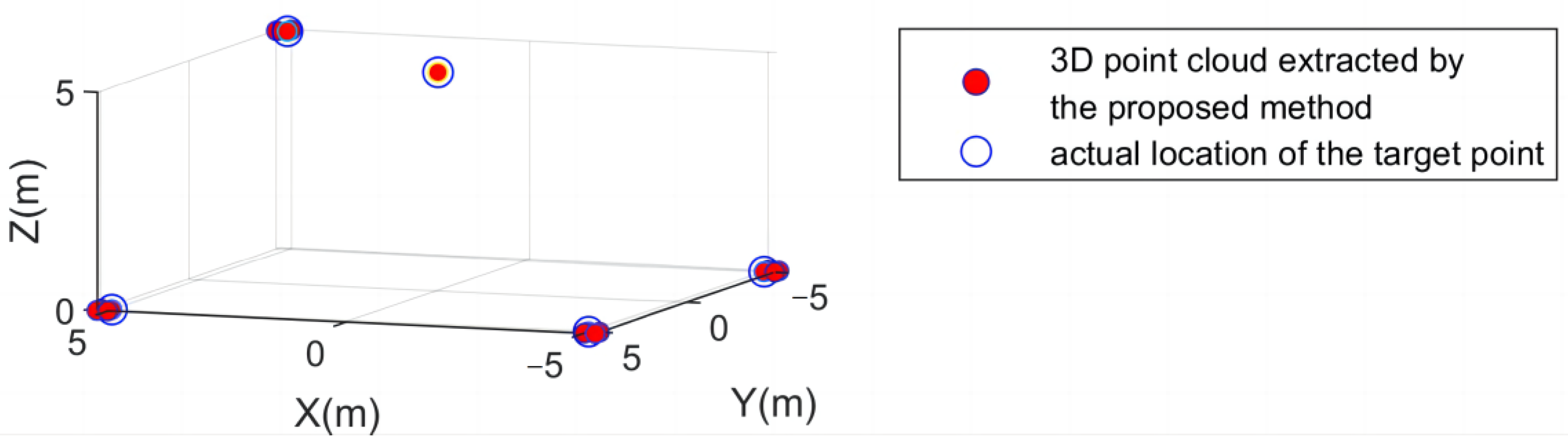
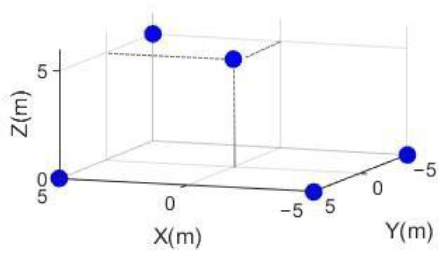
| Serial Number | X (m) | Y (m) | Z (m) |
|---|---|---|---|
| 1 | 0 | 0 | 5 |
| 2 | 5 | −5 | 5 |
| 3 | −5 | 5 | 0 |
| 4 | −5 | −5 | 0 |
| 5 | 5 | 5 | 0 |
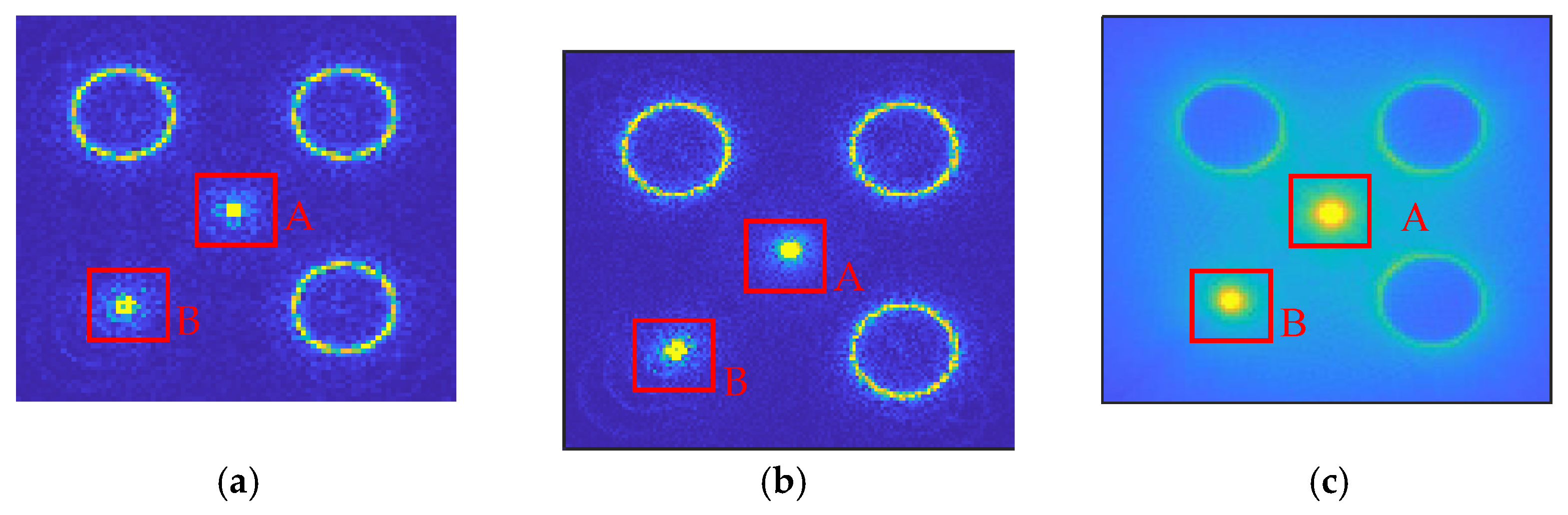
| BP (m) | IBP (m) | The Proposed Algorithm (m) | |
|---|---|---|---|
| point A | 0.2 | 0.24 | 0.36 |
| point B | 0.3 | 0.32 | 0.36 |
| BP (s) | IBP (s) | The Proposed Algorithm (s) |
|---|---|---|
| 3787.4 | 1278.4 | 582.1 |
| BP (s) | IBP (s) | The Proposed Algorithm (s) |
|---|---|---|
| 23,974.43 | 8001.40 | 3809.32 |
Disclaimer/Publisher’s Note: The statements, opinions and data contained in all publications are solely those of the individual author(s) and contributor(s) and not of MDPI and/or the editor(s). MDPI and/or the editor(s) disclaim responsibility for any injury to people or property resulting from any ideas, methods, instructions or products referred to in the content. |
© 2023 by the authors. Licensee MDPI, Basel, Switzerland. This article is an open access article distributed under the terms and conditions of the Creative Commons Attribution (CC BY) license (https://creativecommons.org/licenses/by/4.0/).
Share and Cite
Chu, L.; Ma, Y.; Hao, Z.; Li, B.; Shi, Y.; Li, W. A CSAR 3D Imaging Method Suitable for Edge Computation. Electronics 2023, 12, 2092. https://doi.org/10.3390/electronics12092092
Chu L, Ma Y, Hao Z, Li B, Shi Y, Li W. A CSAR 3D Imaging Method Suitable for Edge Computation. Electronics. 2023; 12(9):2092. https://doi.org/10.3390/electronics12092092
Chicago/Turabian StyleChu, Lina, Yanheng Ma, Zhisong Hao, Bingxuan Li, Yuanping Shi, and Wei Li. 2023. "A CSAR 3D Imaging Method Suitable for Edge Computation" Electronics 12, no. 9: 2092. https://doi.org/10.3390/electronics12092092
APA StyleChu, L., Ma, Y., Hao, Z., Li, B., Shi, Y., & Li, W. (2023). A CSAR 3D Imaging Method Suitable for Edge Computation. Electronics, 12(9), 2092. https://doi.org/10.3390/electronics12092092