Article

Development and Experimental Validation of Control Algorithm for Person-Following Autonomous Robots

by
J. Enrique Sierra-García
1,*,
Víctor Fernández-Rodríguez
2,
Matilde Santos
3,* and
Eduardo Quevedo
1
1
Department of Electromechanical Engineering, University of Burgos, 09006 Burgos, Spain
2
Mova Traffic Engineering, INDRA, 28108 Madrid, Spain
3
Institute of Knowledge Technology, Complutense University of Madrid, 28040 Madrid, Spain
*
Authors to whom correspondence should be addressed.
Electronics 2023, 12(9), 2077; https://doi.org/10.3390/electronics12092077
Submission received: 25 February 2023 / Revised: 21 April 2023 / Accepted: 26 April 2023 / Published: 30 April 2023
(This article belongs to the Special Issue Advances in Autonomous Control Systems and Their Applications)

Abstract

:
Automatic guided vehicles, in particular, and industrial autonomous mobile robots, in general, are commonly used to automate intralogistics processes. However, there are certain logistic tasks, such as picking objects of variable sizes, shapes, and physical characteristics, that are very difficult to handle fully automatically. In these cases, the collaboration between humans and autonomous robots has been proven key for the efficiency of industrial processes and other applications. To this aim, it is necessary to develop person-following robot solutions. In this work, we propose a fully autonomously controlling autonomous robotic interaction for environments with unknown objects based on real experiments. To do so, we have developed an active tracking system and a control algorithm to implement the person-following strategy on a real industrial automatic-guided vehicle. The algorithm analyzes the cloud of points measured by light detection and ranging (LIDAR) sensor to detect and track the target. From this scan, it estimates the speed of the target to obtain the speed reference value and calculates the direction of the reference by a pure-pursuit algorithm. In addition, to enhance the robustness of the solution, spatial and temporal filters have been implemented to discard obstacles and detect crossings between humans and the automatic industrial vehicle. Static and dynamic test campaigns have been carried out to experimentally validate this approach with the real industrial autonomous-guided vehicle and a safety LIDAR.

Graphical Abstract

1. Introduction

Automatic guided vehicles (AGVs) and industrial autonomous mobile robots stand out for their efficiency and versatility in industrial applications [1]. They are autonomous transport vehicles commonly used to replace conveyors and manual industrial trucks in the industrial sector in order to automate the intralogistics processes. They have become even more relevant in the Industry 4.0 framework due to the flexible manufacturing paradigm it entails [2]. These autonomous industrial vehicles provide flexibility, determinism, traceability, and enhance the quality of industrial processes [3,4].
However, there are certain logistic tasks that cannot be or are very difficult to fully automate. For instance, the picking of different parts in racks separated in a workspace. The complexity comes, on the one hand, from the perception abilities required to detect the objects in the rack, sometimes even partially or totally occluded by other objects; on the other hand, from the difficulty of grasping elements of different sizes, shapes, and physical properties. The latter is especially complex in the case of deformable or delicate objects [5].
In these cases, the collaboration between humans and autonomous robots is key in order to carry out these jobs. Humans can perform high-value tasks that are difficult to automate, such as component selection and picking, and the robot can focus on lower-value tasks, such as towing the goods. For this purpose, the autonomous robot must be able to follow the human operator while executing the logistic tasks.
This ability is very useful in many fields and use cases. For instance, a follower cart that transports heavy tools and measurement instruments for a technician, or in hospitals in order to transport medicines and medical devices, or even in supermarkets, autonomously driving the shopping trolley. The latter can be especially useful for people with reduced mobility. Thus, the importance of developing human-following autonomous robots.
In this work, we propose the control architecture and control algorithm for a person-following AGV. The approach can be adapted for any type of AGV or any autonomous robot, no matter the kinematics. In this paper, the control proposal has been experimentally validated on a real hybrid differential tricycle AGV [6] of the ASTI Mobile Robotics company.
The control approach exploits the cloud of points measured with a LIDAR sensor. It allows obtaining the position of the target to be tracked, although other sensing techniques could have been used, such as ultra-wide-band (UWB) [7]. Spatial and temporal filtering has been implemented to discard and avoid undesired obstacles in the surroundings of the target. Indeed, one of the problems of this application is the presence of objects that may cross the path between the sensor and the target. They cause the system to follow them instead of the target and produce unexpected behaviors. To avoid it, a crossing detector has been developed. If the system detects a crossing of something, it waits for a while to check if the crossing is temporal, in which case it continues with the previously registered target, or if a time threshold is exceeded, then it cancels the tracking for the sake of safety. In addition, a speed controller calculates the speed reference, and the well-known pure pursuit algorithm is used to obtain the direction.
As detailed in the state of the art, there are some other previous works related to human-following robots. However, we have tested the approach with a hybrid differential tricycle robot; thus, we have not found equivalent data to perform a numeric comparison. From the qualitative perspective, as the main innovations, it is possible to remark: the dynamic tracking cone to differentiate the target from the surrounding, the crossing detector, the integration of the tracking with the pure pursuit, and the implementation in a hybrid mobile robot.
The rest of the paper is structured as follows. Related works are presented in Section 2. Section 3 explains the model of the AGV and its kinematic equations. The architecture of the control system is detailed in Section 3. Section 4 is dedicated to the study of the person-following algorithm and the generation of the control references for the robot. The results obtained during the static and dynamic experimental tests are discussed in Section 5. Finally, the paper ends with the conclusions and future works.

2. Related Works

People-following is a well-known problem in robotic autonomous navigation. It has a wide range of applications in the home, industry, manufacturing, health care, entertainment industry, and other settings. Different work environments and applications pose various challenges that have been addressed in many ways. In fact, the generation of the appropriate trajectory and the avoidance of collisions are recurring topics in different scenarios. To mention some works in the aerospace field, where they can be critical, in [8] several autonomous trajectory generation algorithms for space robots are proposed, some of them including convex optimization. Raigoza and Sands [9] augmented the previous approach with distributed waypoints for autonomous collision avoidance. The work by Sands [10] uses Pontryagin’s minimization of Hamiltonian systems to derive controls that account for interaction with robot structural dynamics providing autonomous trajectories for highly flexible space robotics. Manikandan et al. (2022) address the problem of AGV tracking of a curve path [11]. They applied model predictive control once the curve had been detected. The so-called curve-aware MPC algorithm has been proven in real-time experiments for mixed environments.
One of the required abilities of AGVs is detection. For security reasons, mainly if they work in congested environments with human operators in the workplace, autonomous vehicles must be able to detect any objects on the path and avoid collisions. This is an issue address for other types of ground vehicles, as shown in the review by Islam et al., 2022. In this case, the paper focuses on ground vehicle detection methods for the off-road environment [12]. Closer to our approach, the paper by Pires et al. (2022) develops an autonomous navigation system for an AGV in order to detect and avoid obstacles based on the processing of data acquired with a frontal depth camera mounted on the vehicle [13]. Zahid and Hao (2022) developed an IoT system for an AGV prototype in an indoor industrial environment. The study produced several significant results related to obstacle detection of AGV with the IoT-based technology that allows flexible wireless communication among mobile robots [14].
The paper by [15] gives a comprehensive overview of the literature on person-following by autonomous robots. The state-of-the-art methods for perception, planning, control, and interaction are discussed, and their applicability in varied ground, underwater, and aerial scenarios is presented. Some of the main challenges of the robotic person-following approaches are also discussed in the survey paper [16] from the social interactions point of view, where the main goal is the design of socially aware person-following robots.
For what concerns terrestrial applications, classifications of the different methods are based on the type of sensors used for perception and on the strategy used to detect the target person, control, and interaction. According to [17], most ground applications use a simple unicycle model that controls the robot’s 2D motion in polar coordinates. The chosen detection system should be able to find the target position and distance from the robot. People are usually localized by means of identification of the face, legs, or whole body by using a laser range finder or 2D imaging sensors.
Nevertheless, most of these works do not address the control of the follower robot as part of the study. Person-following is mainly solved with two main control approaches. The inputs to the robot are synthesized so as to control either the relative position of the robot w.r.t. the person frame or the relative position of the person in the robot frame (person frame-based control or robot-centered control) [18]. This way, the mobile robot is able to follow the leader (human), whether in front, side-by-side, or behind the robot. The cutting-edge communication-control co-design is presented in the paper by Qiao and Yuan (2022) and applied to an AGV [19]. Indeed, this work analyzes and summarizes the existing communication–control co-design methods and shows as a challenging use case the cloud control of an automated guided vehicle (AGV) in a future factory. The paper by [20] covers the review of trends in person-following robot control algorithms, describing different methods where the robot receives input of tracking data and outputs the movement of the robot accordingly. Moshayedi et al., 2022, propose a PID control tuned with different techniques to adjust the difference in the speed of both sides of the robot; thus, the robot will be able to move along the path [21]. They are simulated and tested on different trajectories on a model of the AGV.
In [4], a hybrid controller that combines reinforcement learning-based control (RLC) and PI regulators is applied to solve the trajectory tracking control and the longitudinal velocity control of an AGV.
Reis et al. (2022) detect the gap in the literature on control strategies of the position of AGVs [22]. The paper proposes a systematic literature review to investigate the research field from the controller design perspective, and the technological tendencies of the proposed solutions are revealed.
In [23], a Lyapunov globally asymptotically stable controller is proposed, where the human user velocity is also taken into account to modify the controller gains. It also addresses the extended kinematic and the inverse kinematics model-based controller for the differential-drive mobile robot. A non-linear controller is proposed in [24] focused on the so-called jack-knife effects to avoid the limitation of classical control laws regarding the robot’s non-holonomy and the difficulty of estimating the person’s orientation. In [25], the robot follows the operator from behind by feeding decentralized proportional or PID controllers with relative and translational errors to the robot. Petrov et al. (2021) address the control of an autonomous mobile robot when it is following a person in front of him. Using a leader–follower formation approach combined with a look-ahead concept, a human-robot kinematic model in error coordinates with respect to a local Cartesian coordinate system is developed [26]. Non-linear feedback control is designed using local information from the onboard sensor for the relative human–robot position and orientation. An adaptive control is proposed to estimate the unknown human linear and angular velocities.
The paper by Oh-hara, 2022, presents an image-based control for a person following a mobile robot [27]. Based on the estimate of the lowest positions of both feet of a tracked person through particle filters based on color invariances, authors control the velocity of the robot. They define an analytic control law using the image coordinates so it coincides with the target point.
The longitudinal control scheme of a person following a robot usually aims at keeping a specified distance during the following. It could be approached with classical regulators, such as PID [28], or with more sophisticated or intelligent techniques. In [29], an intelligent control based on fuzzy logic is proposed. It makes use of a laser range finder mounted on a wheeled mobile robot to detect and follow a person’s legs while keeping a safe distance. The fuzzy system has two inputs, the relative velocity of the robot to the person’s legs and the difference between the relative distance and the safe distance. The output is the needed acceleration of the robot. Another fuzzy logic control strategy is proposed in [30] to obtain the appropriate velocity of the following robot. The gap between the person and the robot is used, and the longitudinal direction is obtained. In [31], the challenges of the person-following robot longitudinal control are summarized, including reverse, gap range, no imitation, and the leader person’s periodic/random movement. Then the person-following robot longitudinal control based on the data of the bar-laser-perception device is presented.
Finally, in [32], a contactless control system for an automatic guide vehicle (AGV) is developed. The AGV is designed using a tricycle drive system. Using a depth camera, the AGV is programmed to be able to follow human movements without marking or direct contact.
So, as far as we know, the human-following approach is not so common in the industry environment, and the related literature does not usually include AGVs, nor address the control problem for these vehicles in the follower configuration.

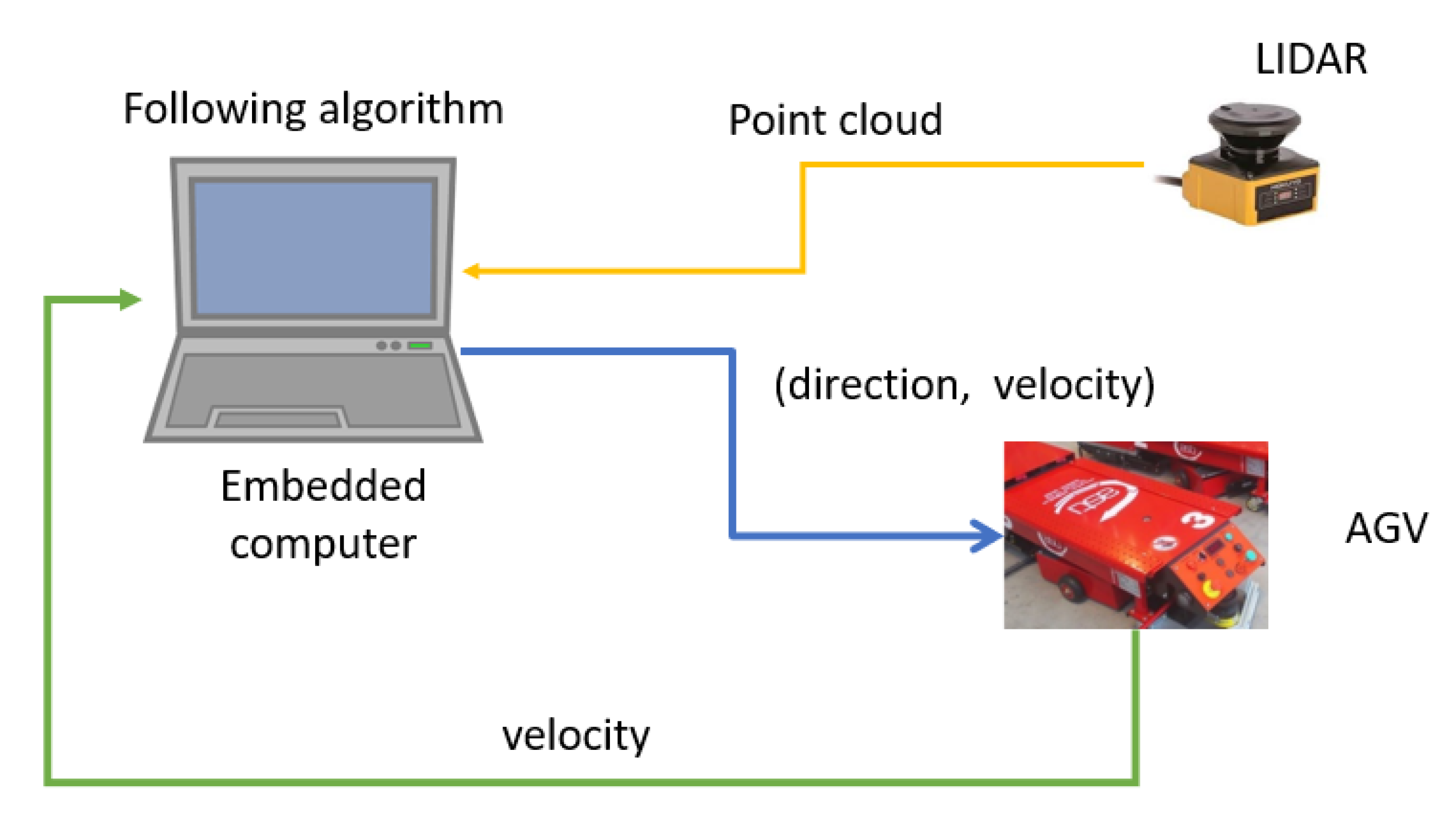
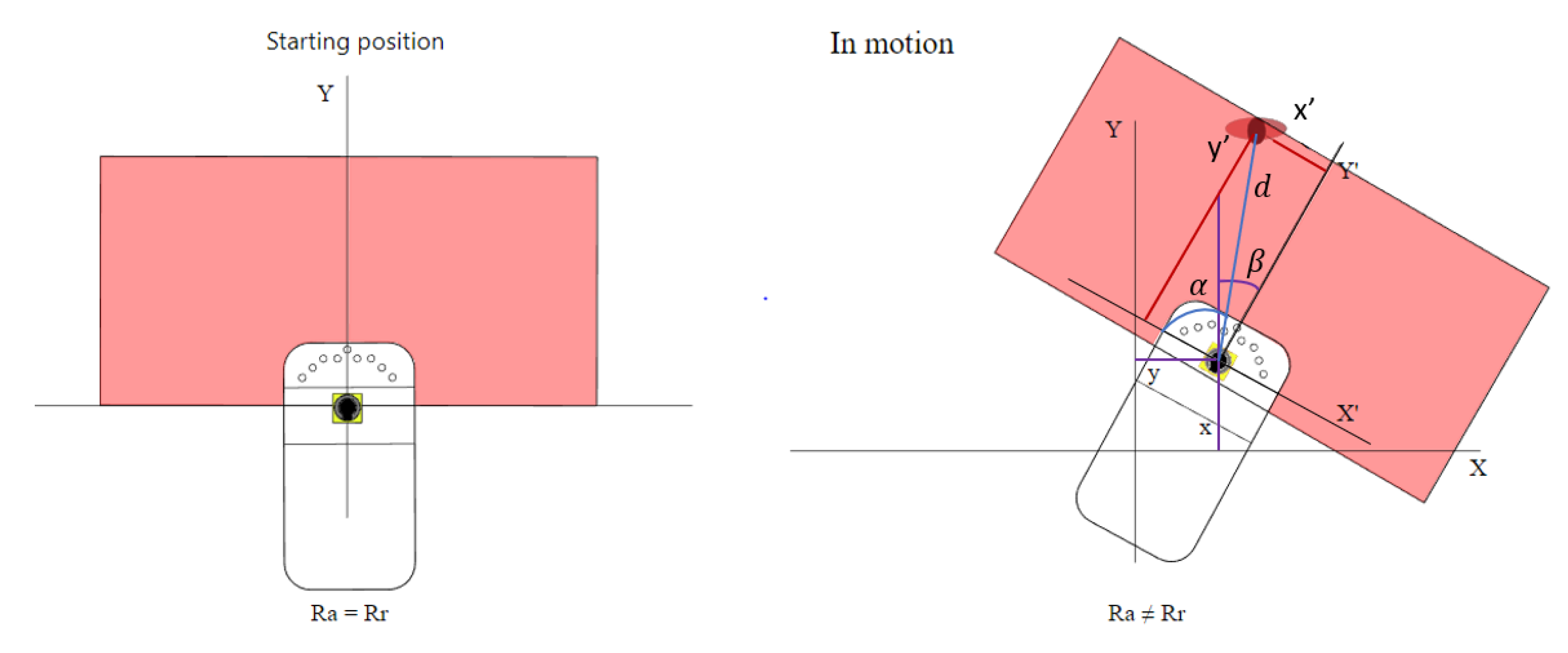
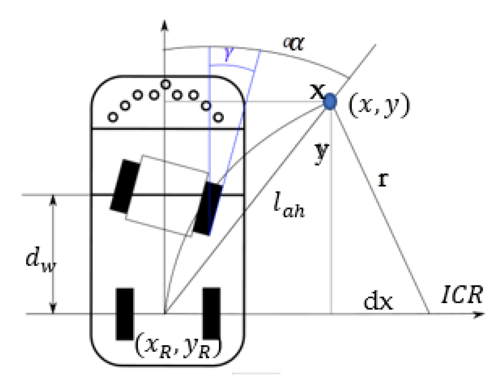
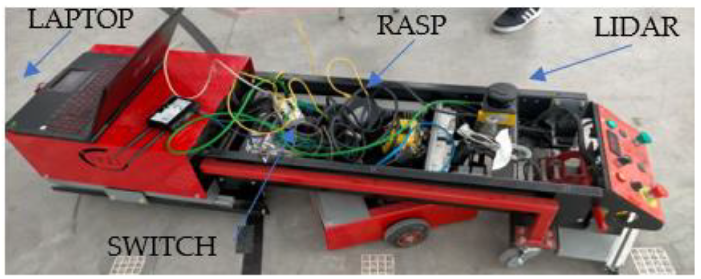
3. Model of the System

The here proposed human-following controller can be implemented in any type of AGV or any autonomous robot. However, in this work, we have used a hybrid tricycle and differential tow AGV. This type of hybrid autonomous guided vehicle is widely used in the industry. The traction unit works as a differential mobile robot. This traction unit is linked to the body by an axle on which it pivots. Thus, the kinematics of the AGV body follows the movement of a tricycle robot. Figure 1 shows a schematic representation of this hybrid AGV.
The kinematic model of the AGV is described by Equations (1)–(3). These equations are explained in more detail in [33,34].
x ˙ h = V L + V R 2 cos Φ h ,   y ˙ h = V L + V R 2 sin Φ h ,   Φ ˙ h = v R v L L h
x ˙ b = v h cos γ cos Φ b ,   y ˙ b = v h cos γ sin Φ b ,   Φ ˙ b = v h L b sin γ
v h = x ˙ h 2 + y ˙ h 2 = v L + v R 2
where x h , y h , Φ h and x b , y b , Φ b denote the position (m) and orientation (rad) of the body and the traction unit, respectively. The variable v h (m/s) is the longitudinal velocity of the traction unit, L h (m) is the distance between the wheels in the traction unit, L b (m) is the distance between the rear wheels and the center of the traction unit, v L is the linear velocity of the left wheel, and v R is the linear velocity of the right wheel.
Normally, in these types of AGV, the control references are v L and v R . However, in the AGV used in the experiments, there is an embedded controller for the wheel speed and a control interface such that the external references are the longitudinal velocity v r e f and the direction, γ r e f , as shown in Figure 1. These external references v r e f ,   γ r e f   are internally transformed into wheel speed references by Equations (4)–(6).
w r e f = Kp w γ r e f γ + Kd w d γ r e f γ d t + KI w γ r e f γ d t
v L R E F = v r e f w R E F · L h 2
v R R E F = v r e f + w R E F · L h 2
The parameters of the model are summarized in Table 1.

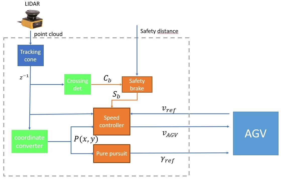
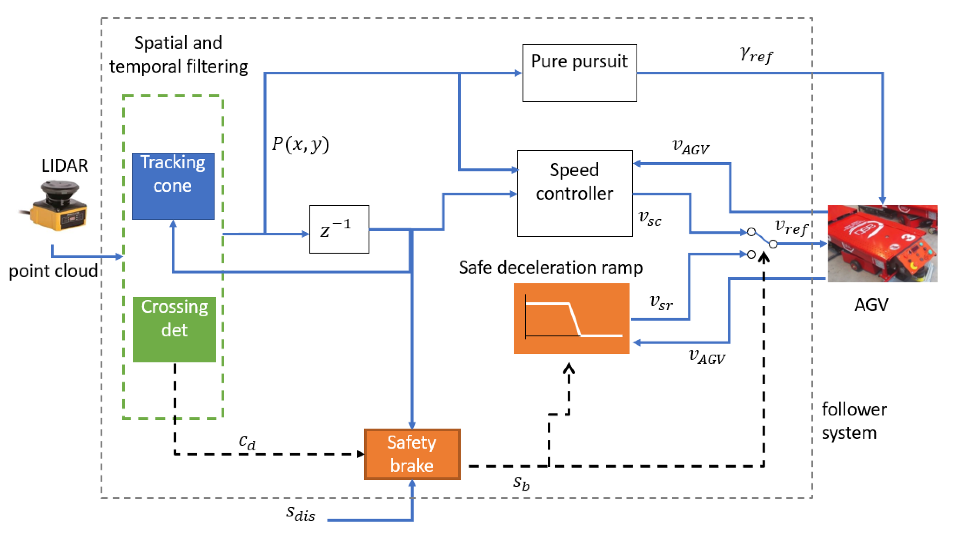
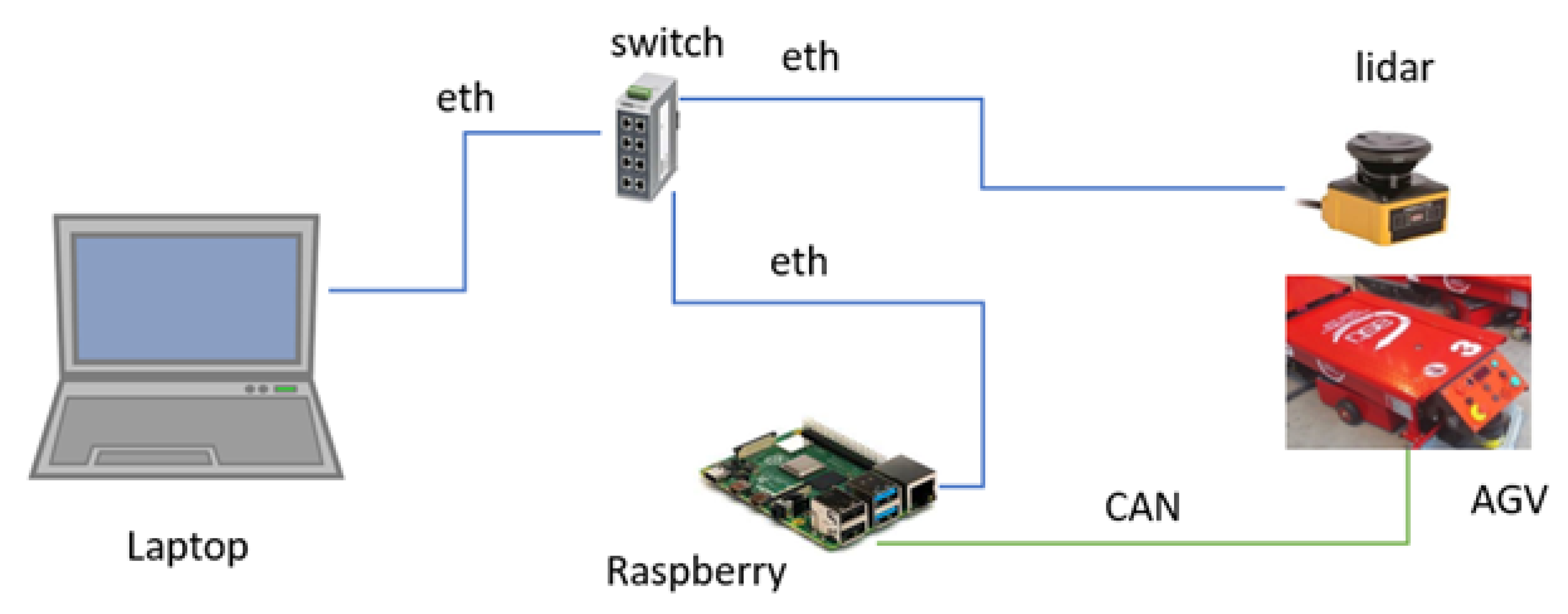
4. Description of the Control Architecture

Figure 2 shows the hardware control architecture. A safety LIDAR gives a cloud of points to an embedded computer. This computer oversees the detection of the target, performs the tracking algorithm, and obtains the control references sent to the AGV. Depending on the AGV type, the control references can be given as pairs (direction, velocity), (angular velocity, longitudinal velocity,) or (left velocity, right velocity). In this work, we use an AGV that is controlled by the direction and the speed. In turn, the AGV provides information to the embedded computer about its current velocity. If this information is not available, for instance, in the case the AGV is not equipped with encoders, this speed could be estimated from the previous speed references.
The software configuration of the person-following system is shown in Figure 3. The point cloud obtained by the LIDAR goes to the module in charge of the spatial and temporal filtering. This module selects the correct samples of the lidar for the right-tracked target. It is composed of a tracking cone (spatial filter) and a crossing detector that acts as a temporal filter. Both are further explained in Section 4. The crossing detector also generates a signal to trigger the safety brake, c d , if a crossing is detected.
The position of the target detected, P(x,y), feeds the input of the pure pursuit algorithm and the speed controller. Pure pursuit generates the reference of the direction, γ r e f , for the AGV. The speed controller also receives the position of the target in the previous iteration. The current position and the previous one are used to estimate the speed of the target. Then the pure pursuit calculates the speed reference for the AGV to follow the target, v s c . When the AGV is working, this speed reference is used as a reference for the AGV, v r e f (switch of Figure 3 in the upper position).
In case the distance to the target is below the safety distance or when a crossing is detected ( c d = 1 ) the safety brake module triggers the safety stop, s b = 1 . This event changes the switch to the down position, then the speed reference given by the safe deceleration ramp, v s r , is used, and the AGV stops in a controlled way. It is important not to confuse this stop managed by the human-following controller with the stop commanded by the AGV safety system. Indeed, to ensure that both safety systems coexist well, it is necessary to set the safety distance of the human-following architecture larger than the safety distance of the safety device embedded in the AGV.

5. Human-Following Algorithm

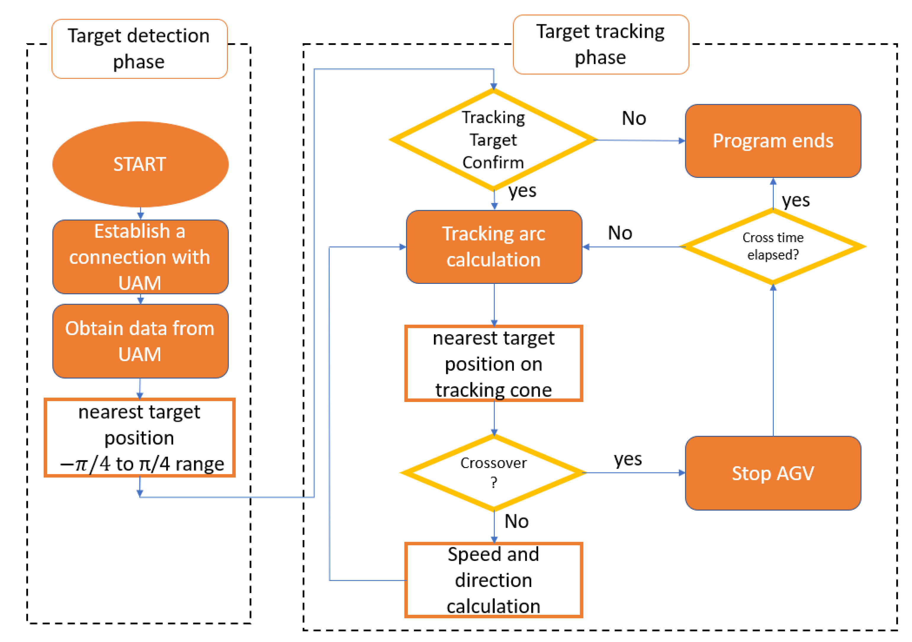
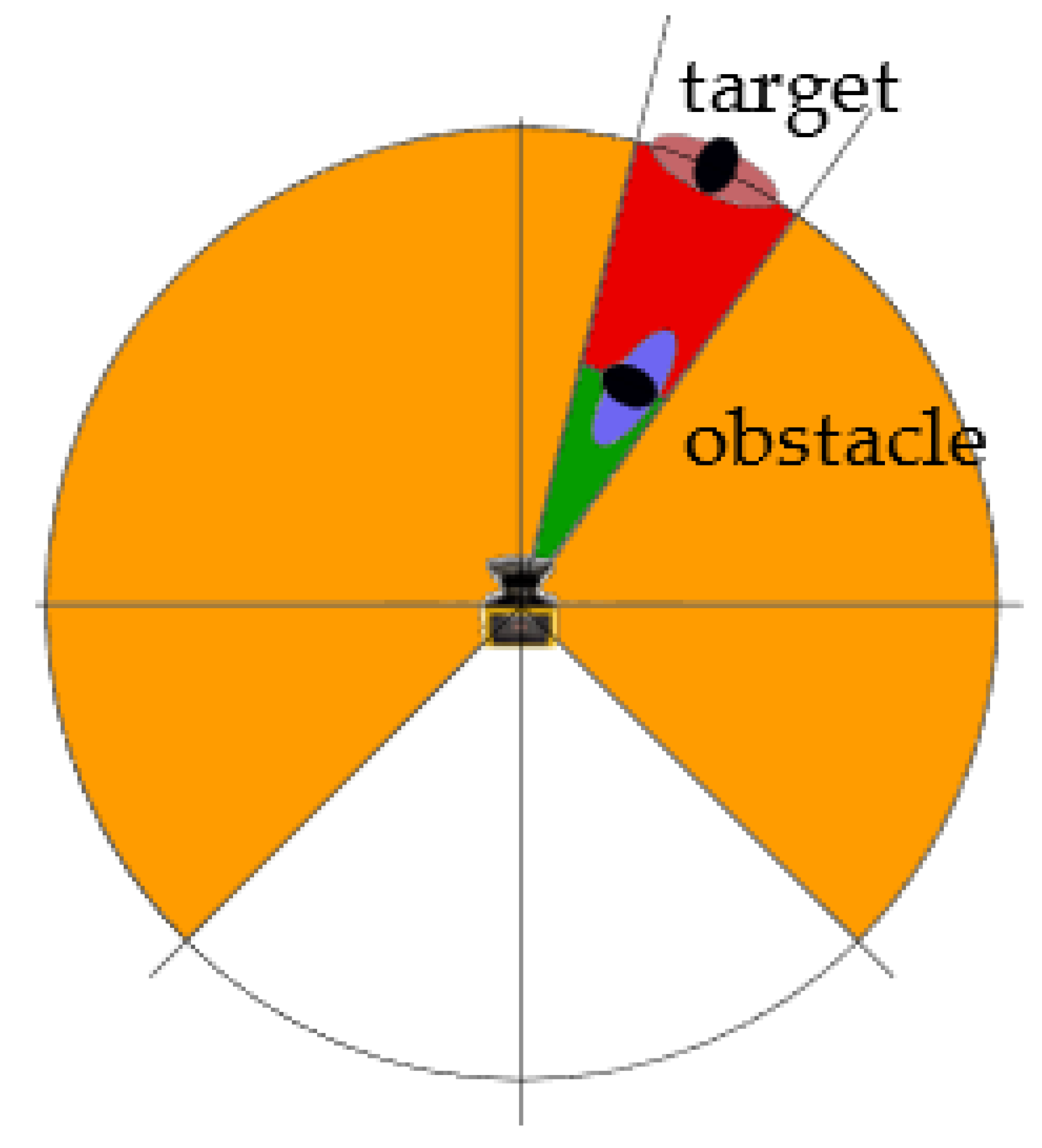
5.1. General Description

The flowchart of the person-following algorithm is shown in Figure 4. It is structured in two phases: detection and tracking. It starts with the detection, and once a target is detected and confirmed, it moves to the tracking phase.
During the initialization of the process, the industrial computer where the algorithm is running must establish a connection with the lidar sensor to receive the scans. Then the algorithm waits to detect a target in the initial tracking cone. As it is explained in the next section, during the detection phase, the range of the detection cone is ( π 4 , π 4 ) . Samples outside this range are initially filtered.
Once a target is detected, the system requests confirmation from the operator before tracking the target. If the operator declines the tracking, the process ends; otherwise, the algorithm goes on to the tracking phase. Usually, there is no need for two persons to do this, the followed human and the operator. In industrial workspaces, it is expected that people use an app to see the objects perceived by the AGV and confirm that he/she is the correct tracking target. After this confirmation, the application sends a command to the AGV to start the tracking process. This can be observed in Figure 4.
While in the tracking phase, the algorithm calculates the circumference arc required to reach the target. Then it obtains the nearest target position within the tracking cone to track the movement of the object and to detect if an obstacle has crossed between the target and the lidar. If there is a crossing, it stops and checks if it is an instantaneous or a permanent crossing. If the obstacle remains after the crossing threshold time, the program ends. Otherwise, if the crossing disappears, the algorithm calculates the speed and the direction references and calculates the circumference arc again to the next point. This process is carried out continuously until a permanent crossing is detected or the operator decides to stop the tracking.
The operation of the human-follower robot described in Figure 4 can be formalized by Algorithm 1. In this algorithm, r e a d L I D A R ( ) is a function that gives the measurements of the LIDAR in polar coordinates r , θ , where r denotes the distances, and θ represents the angles. The function f i l t C o n e is the filtering cone; it receives the distances and the angles measured by the LIDAR and filters them to obtain the measures that belong to the tracking cone. This is further explained in Section 5.2.1. The function g e t M I N ( ) calculates the closest point r m i n , θ m i n of the filtered point cloud, r f , θ f . The function p o l a r 2 C a r t ( ) transforms polar coordinates to cartesian coordinates, and it is used to calculate the position of the closest point in cartesian coordinates x m i n , y m i n . The function g e t C o n f i r m a t i o n () shows the detected position to the user and requests confirmation for the tracking.
The crossing detection is implemented by the function c r o s s i n g D e t e c t i o n ( ) , that generates the crossing condition, c d , and updates the latest position, r o k , if there has not been an obstruction. The elapsed time t c d is used to measure the duration of the LIDAR obstruction. This is further explained in Section 5.2.3. The velocity reference and direction reference are obtained by the functions u p d _ V r e f   and u p d _ Υ r e f , respectively. They are detailed in Section 5.3.1 and Section 5.3.3. Finally, the function that updates the detection cone is called u p d cone (see Section 5.2.2.)
Algorithm 1. Human-following algorithm.
c o n f     F A L S E
   t c d     0
   c o n e     45 ,   45
 
   While { t   < T e x e c }{%Detection phase
       While { c o n f   = F A L S E }{
          r , θ   r e a d L I D A R ( )
          r f , θ f   f i l t C o n e r , θ , c o n e
          r m i n , θ m i n   g e t M I N r f , θ f
          x m i n , y m i n   p o l a r 2 C a r t r m i n , θ m i n
          c o n f   g e t C o n f i r m a t i o n x m i n , y m i n
          x o l d , y o l d , r o k x m i n , y m i n , r m i n
      }end While
      While { t c d <   T c }{ %Tracking phase
          r , θ   r e a d L I D A R ( )
          r f , θ f   f i l t C o n e r , θ , c o n e
          r m i n , θ m i n   g e t M I N r f , θ f
          x m i n , y m i n   p o l a r 2 C a r t r m i n , θ m i n
          [ c d , r o k ]   c r o s s i n g D e t e c t i o n r o k ,   r m i n
          If c d = 1 then
             v r e f   = 0
             t c d   =   t c d + Δ t
          Else{
             t c d     0
             v r e f   u p d _ V r e f x o l d ,   y o l d , x m i n ,   y m i n
             v r e f   u p d _ Υ r e f x m i n ,   y m i n
             c o n e   u p d _ c o n e θ m i n
         }End If
          x o l d x m i n
          y o l d y m i n
       }end While
  }end While
The detection cone is initially set to cover 90° centered at 0°, from −45° to 45°. The crossing time counter is initialized to 0. The algorithm is divided into two parts. First, it measures the closest point and waits for confirmation from the user. This is done continuously until the confirmation is received, and then it starts the tracking phase. In this second phase, it first obtains the closest point and checks whether this point is a crossing object or not. If it is a crossing object, the AGV stops and updates the crossing time counter. In the next iteration, it measures the closest point again and checks if the crossing persists. If the crossing event takes longer than Tc, the tracking phase finishes and goes back to the detection phase. On the other hand, when no crossing is detected, the crossing time counter is reset, and the control references and the tracking cone are updated.

5.2. Target Detection, Filtering, and Tracking

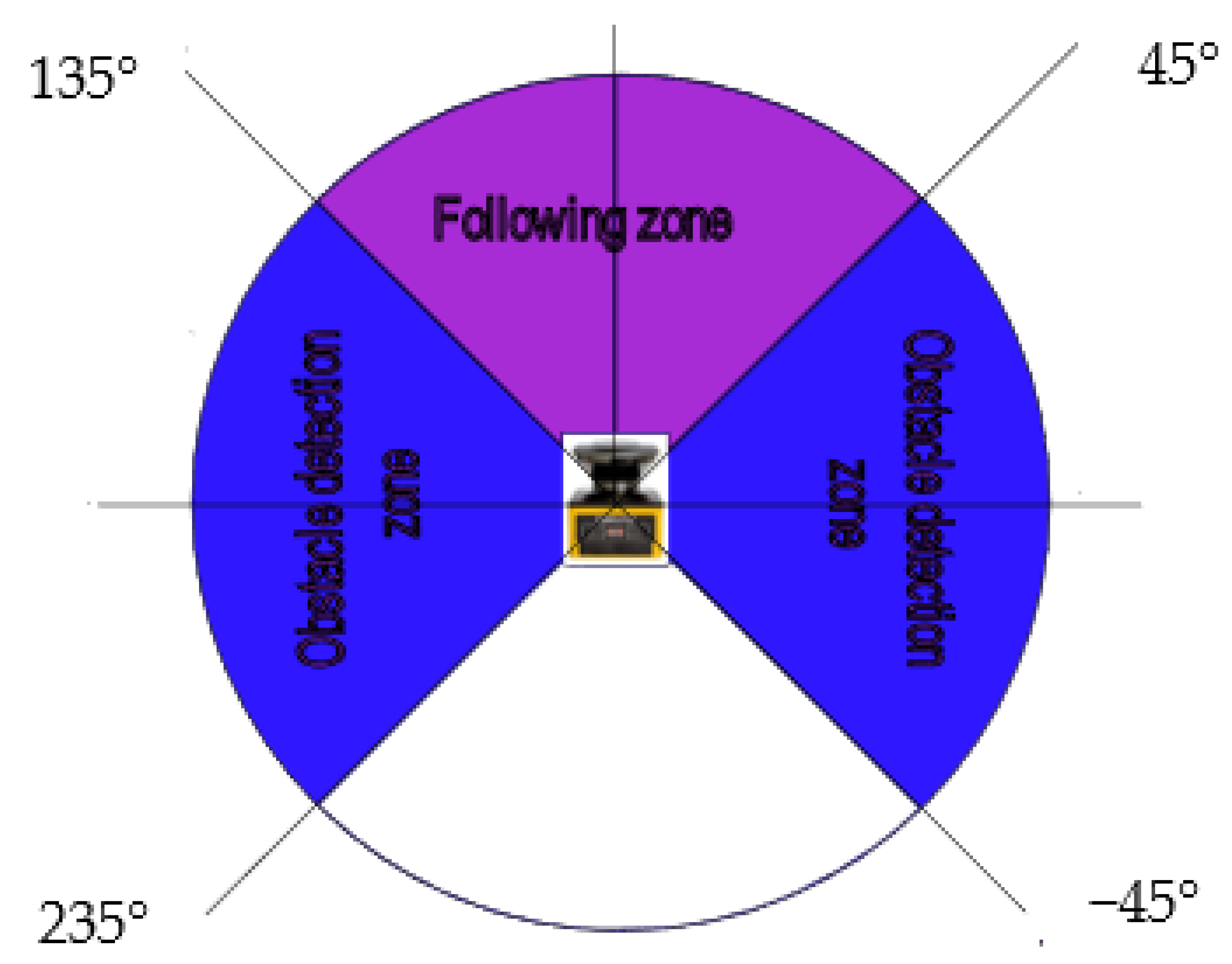
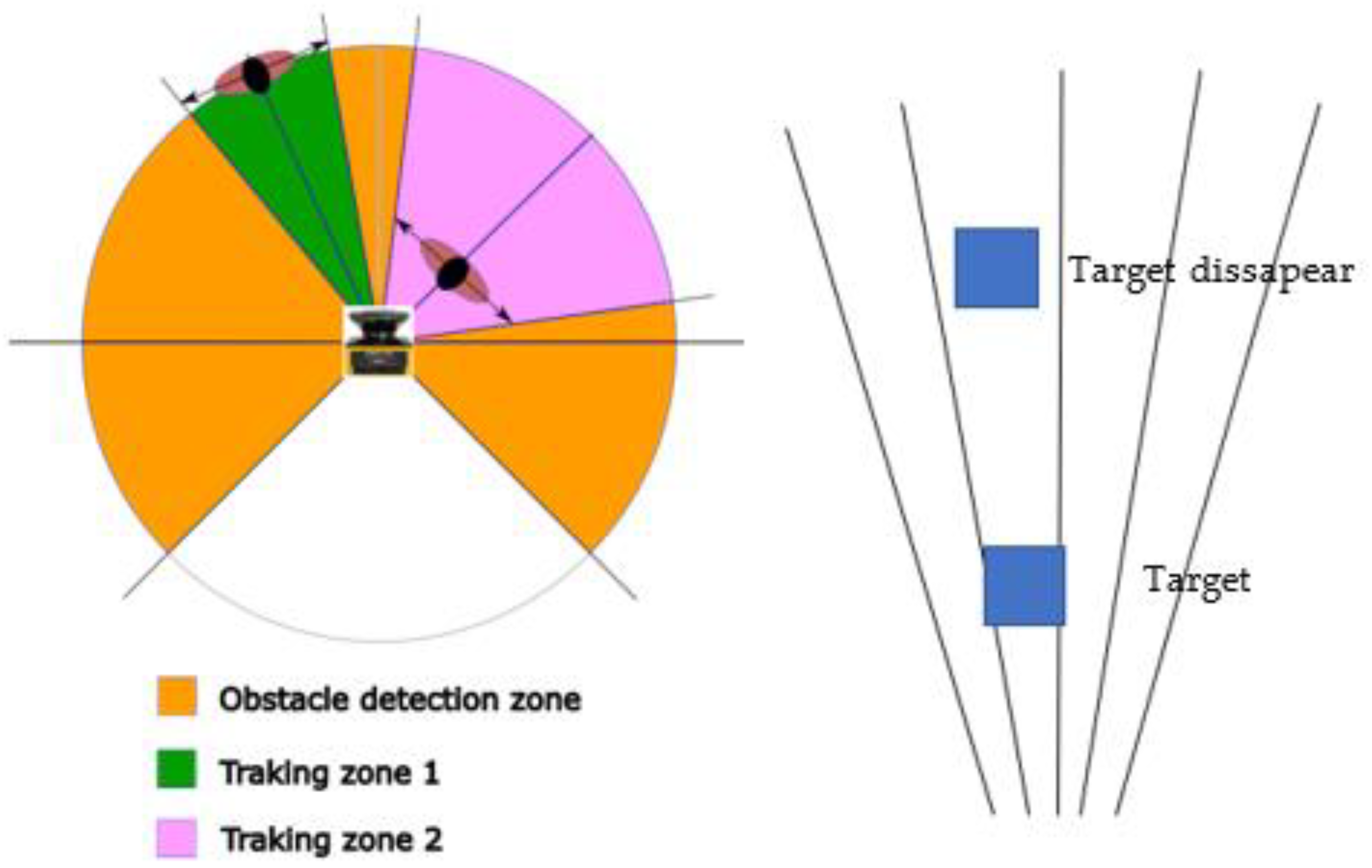
5.2.1. Target Detection

When the algorithm starts, it must detect the object or person to be tracked. To do so, the algorithm performs an initial sweep and compares all distances obtained. The algorithm identifies the target as the point closest to the lidar.
It is noteworthy to clarify that during the object detection phase, a filter is applied to reduce the scan range of the lidar. The laser has a sweeping range of 270°, which, in the case of our setup, only leaves the rear of the AGV uncovered (the scanning device is a safety lidar). However, for object detection and tracking, we must consider that the object to be tracked will be mainly and most of the time in front of the AGV. This way, we can reduce the cone to 90° around the front of the scan during the object detection phase. This filtering is represented in Figure 5.
When the human (target) is detected by the system, the human operator must confirm that he/she wants to be followed by the AGV. This confirmation is key to avoiding the AGV following undesired people or objects.
The adjustment of the angle of the field of vision, α f o v , must consider the clearance to the lateral obstacles, s c . If this angle is not well configured, the LIDAR could perceive the lateral obstacles closer than the human target and would not follow the human. The following Figure 6 shows the situation when the AGV must track a human in the presence of lateral obstacles in the surroundings.
The distance to the obstacle is denoted as l o . In this situation, in order to enable human tracking, the condition l o > l a h must be satisfied. By performing some trigonometrical operations, it is possible to obtain the constraint of the field of vision.
l d > l a h = > w b + s c cos π 2 α f o v 2 > l a h = > α f o v < π 2 acos w b + s c l a h
In our case, the width of the AGV is 50 cm, so w b = 25 cm. If we consider a safety clearance of s c = 50 cm, the field of vision constraint is α f o v < 97.18°. As we have used an angle of 90°, the field of vision meets the constraint.
From another perspective, by operating the previous equation, it is also possible to obtain the minimum safety clearance for a given field of vision.
s c > l a h cos π 2 α f o v 2 w b

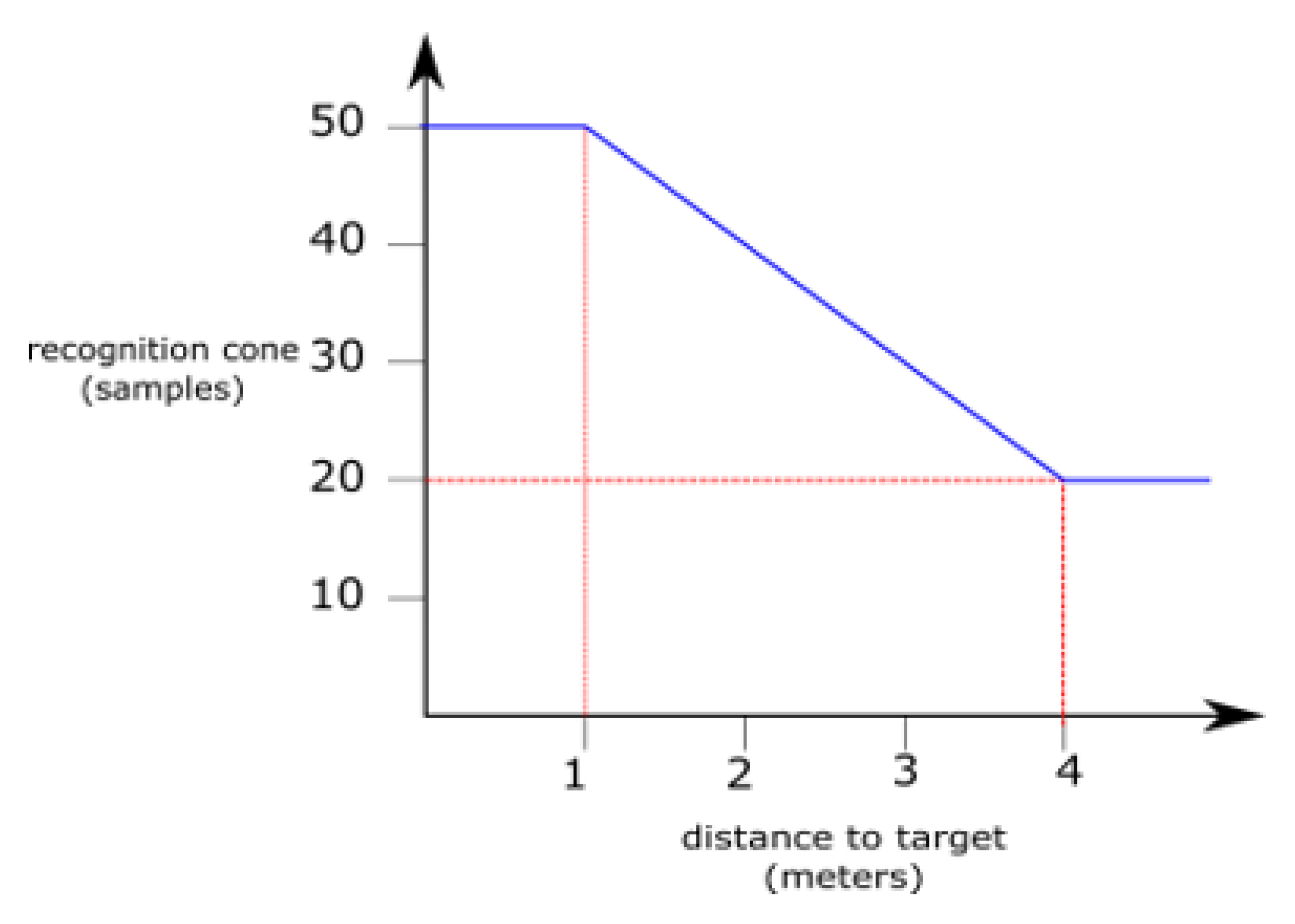
5.2.2. Target Tracking

Once the target has been detected, the system must follow it, avoiding mistaking it for other possible objects within the detection field. With this aim, in this approach, we have reduced the detection cone even further than shown in Figure 5. Even more, the detection cone moves with the object. This dynamic spatial filtering is based on three main assumptions:
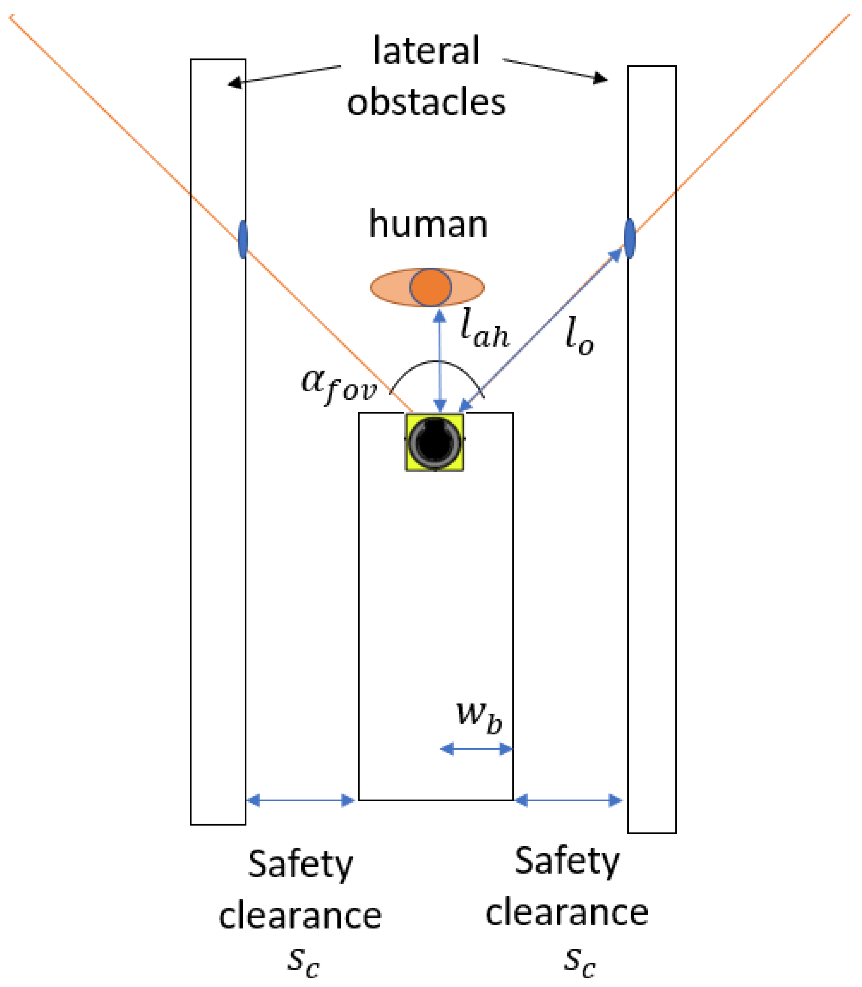
  • The human to be tracked has a detectable thickness greater than 10 cm;
  • The human to be tracked does not move at too high a speed; we can assume that it is not higher than 1.5 m/s;
  • The laser has a scanning frequency of 30 ms, so it performs about 33.3 scans per second.
According to these assumptions, when the target moves at the maximum speed of 1.5 m/s, it travels 4.5 cm during a lidar sweep, that is 30 ms. Therefore, it does not make sense to search for the object outside this range of motion. In this way, we reduce the detection field to the object’s surroundings. However, to consider a certain clearance, we extend this margin to 20 cm per scan. For a proper operation, the distance between the legs of the worker and other objects must be larger than 4.5 cm. The previous assumptions have been specified for human-following robots; however, they could be updated to follow other different tracking targets.
As the laser makes a circular scanning, the perimeter of the circular sector scanned grows with the distance. However, the number of samples scanned only varies with the angular range; it is not affected by the distance. Therefore, if a target is detected by n samples of the lidar at a certain distance, it will be detected by n / 2 samples if the distance is doubled. That is, the number of samples scanning the target is inversely proportional to the distance. From another perspective, the distance between two consecutive samples grows with the distance; thus, the measurement error also grows. Indeed, if the distance is large enough, the detected target could disappear between two samples (Figure 7 right). On the other hand, if the target approaches the lidar, we must increase the detection cone if we want the target to be totally covered by the scan (Figure 7 left).
In order to avoid false readings, it is necessary that several samples simultaneously scan the target. We have set the number of samples to detect the target to 5. Thus, if the target measures 10 cm, then the minimum distance between samples is 2 cm.
The capacity to differentiate two objects that are very close depends on the distance between two lidar samples, so it is possible to obtain the distance between samples, d s , as a function of the distance r from the center of the lidar (Equation (9)).
d S r = 2 π r 3 4 N s p s  
where N s p s is the number of samples per scan (a technical parameter of the LIDAR), and r is the distance from the LIDAR to the object. Considering the perimeter of the circumference, the angular range of the lidar (270°), and that in the experimental implementation, N s p s = 1080, at 1 m this distance d S is 0.43 cm. So, the LIDAR would be able to distinguish two objects even if the distance between them is smaller than 4.5 cm.
From this equation, it is possible to check that if we want to obtain a distance between samples less than 2 cm, the radius must be less than 4.583 m, i.e., around 4 m. At this distance from the lidar, the distance between samples is d S = 1.7453 cm, so we need 11.46 samples to cover 20 cm. To guarantee some clearance, we set this value to 20 samples.
We defined the minimum distance from the lidar as 1 m so the AGV is able to brake in time if an obstacle appears. At 1 m, the distance between samples is d S = 0.436 cm; thus, to cover a displacement of 20 cm, it is necessary to have 45.83 samples, which we round to 50 to simplify the calculations.
Considering these values, it is possible to draw a function that represents the evolution of the samples that we must consider in the detection cone with respect to the distance from the lidar (Figure 8). The lowest limit is (1, 50), and the highest limit is (4, 20); these two points are linked by a straight line.
Figure 8 can be mathematically described by Equation (10):
n s r = 50 , r 1 10 r + 60 , 1 < r < 4 20 , r 4  
As the target can move in both directions, the width of the detection cone at a distance r is given by 2 n s r in a number of samples.
The algorithm selects the target to track (the closest point to the lidar), denoted by s m i n ,   r m i n , where s m i n is the number of samples, and r m i n is the distance to the target. The distance r m i n is used in Equation (8) to obtain n s . This n s value allows it to obtain the range of the detection cone in samples s m i n n s ,   s m i n + n s . Using this dynamic spatial filter, we can keep tracking the target even if an obstacle appears closer to the laser than the selected target, for example, when passing near a wall (Figure 9).
This tracking process is performed by the algorithm every scanning cycle, i.e., about 33.3 times per second at maximum speed, so ensuring that the target is not missed.
In addition to the tracking cone, a further step has been taken to prevent the laser from missing the target in case of an object crosses between the laser and the target, the cross detector.

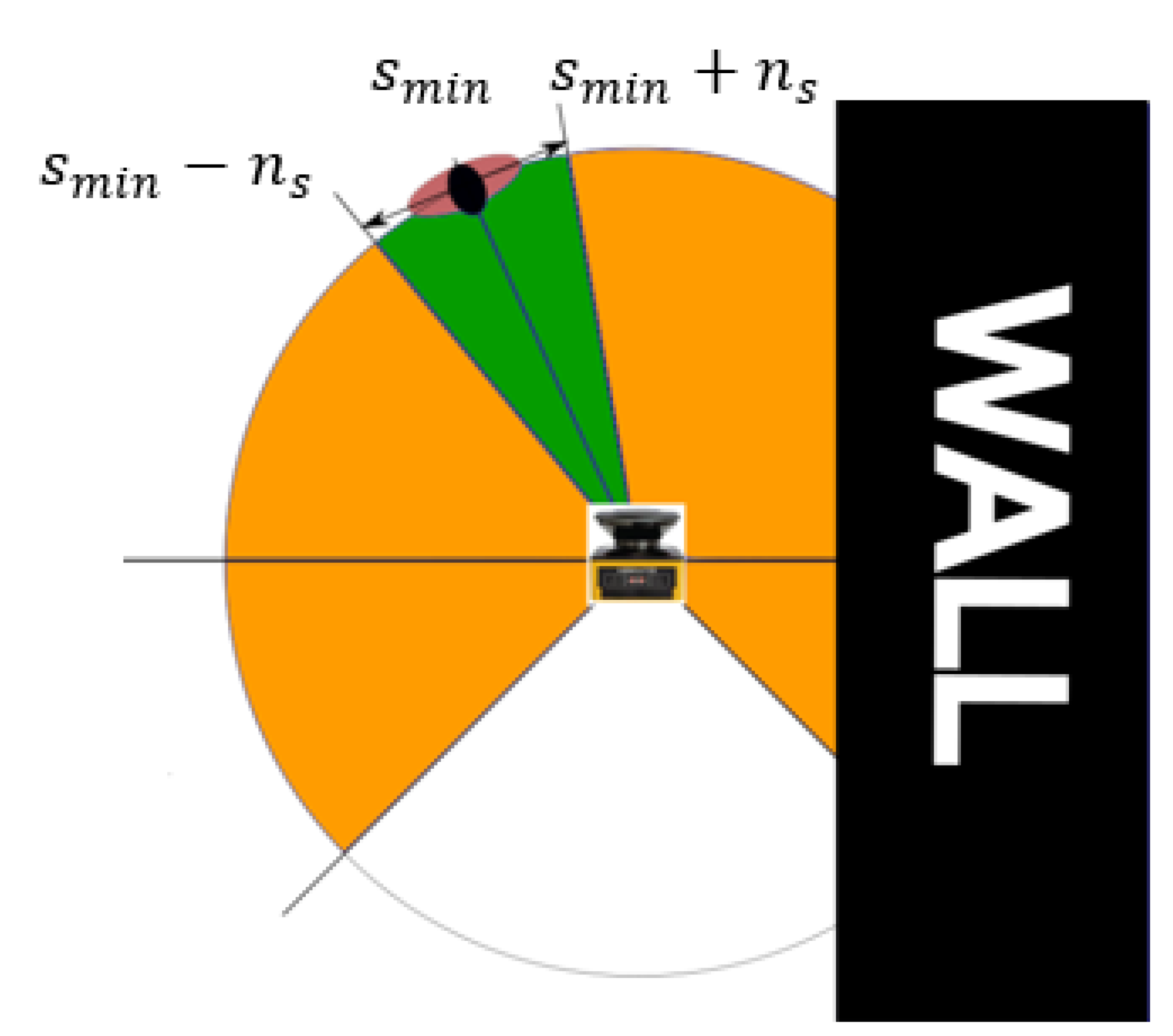
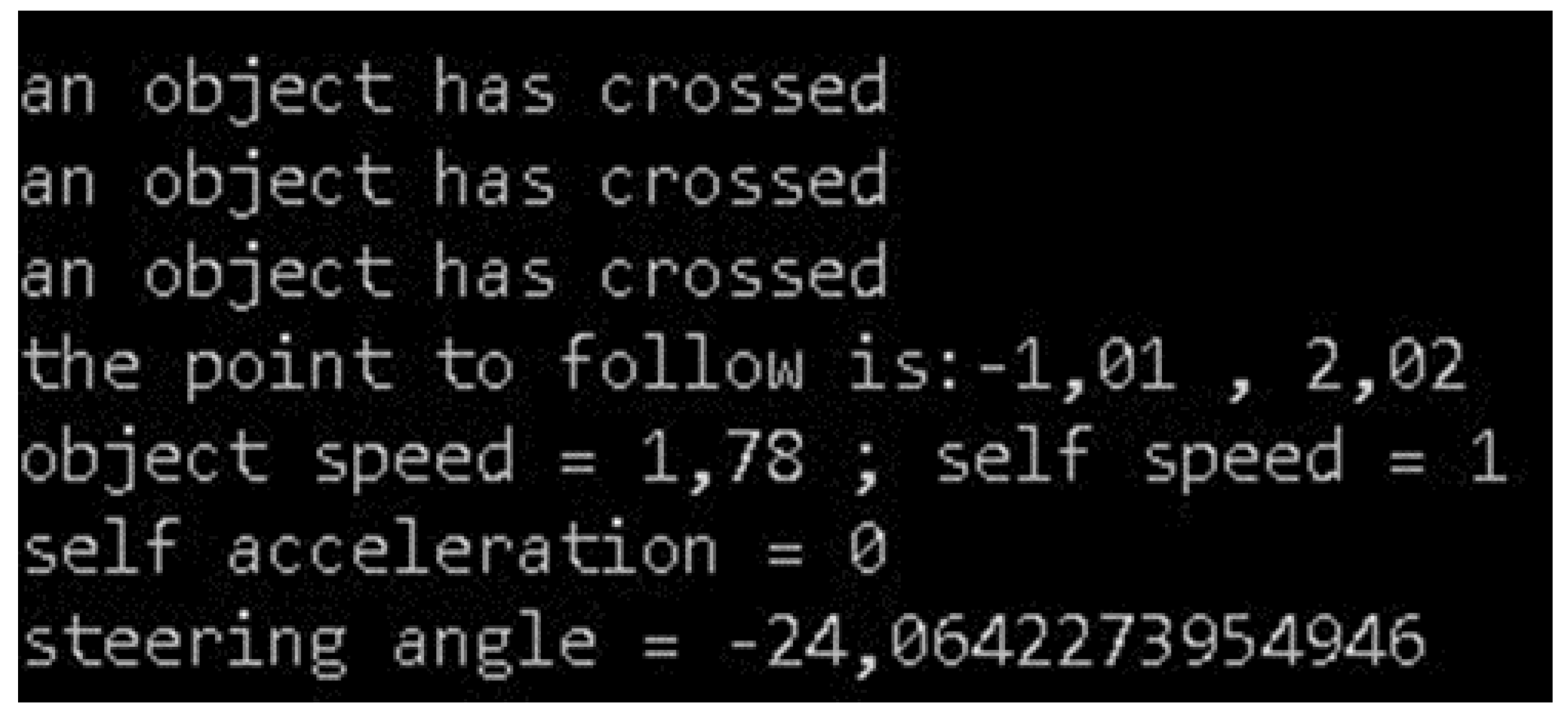
5.2.3. Crossing Detection

One of the main problems that can be found while tracking a target is that an obstacle crosses between the AGV detection cone and the target. So far, the algorithm is vulnerable to this possibility since it could detect this obstacle as the closest object to track. Fortunately, this event can be detected and filtered. This is represented in Figure 10.
Considering that the AGV always keeps a safe distance from the target, we can assume that the crossing will not occur closer than that distance to the target. Then, if the algorithm perceives a difference between two consecutive scans larger than a certain distance d c , and the detected point is closer to the lidar, there is a high probability that an object has crossed. This behavior is similar to a low pass filter, and it can be formalized by Equation (11).
c d t i , r o k t i = 1 ,     r o k t i 1 , r o k t i 1 r m i n t i > d c 0 ,     r m i n t i , o t h e r c a s e
When this happens, the best alternative is to stop the AGV to avoid any collision. However, there may be occasions when the crossing is only momentary or the laser gives a false positive. To solve that, a standby mode that is activated when a crossover is detected is included in the algorithm. When so, the AGV will slow down, but the program will continue to search for the original target it was following. Once the obstacle has passed, the search for the target continues within the detection cone, comparing the distances obtained with those before the crossing. If the target has not moved more than d c , the program will recognize it again as the target to follow and will continue to run normally. During the experimental tests, the distance d c was set to 20 cm.
When a crossing happens, it may cause the crossing object to be considered the original tracking target. To solve it, our algorithm defines a configurable crossing time parameter, T c . This way, if this obstruction time is less than T c , the crossing obstacle is considered a momentary crossing or a false positive. In this case, the tracking of the initial target continues. However, if the crossing time is longer than T c the algorithm stops, and the user must start the tracking process again. This is done for safety reasons as if the lidar is obstructed for a long period, the initial tracking target could have changed its position or been replaced by an unexpected object. All the variables and parameters that are used in target tracking are shown in Table 2. With this safety mechanism, we avoid following undesired crossing targets. This procedure is presented in the flowchart of Figure 4.

5.3. Generation of Control References for Velocity and Direction
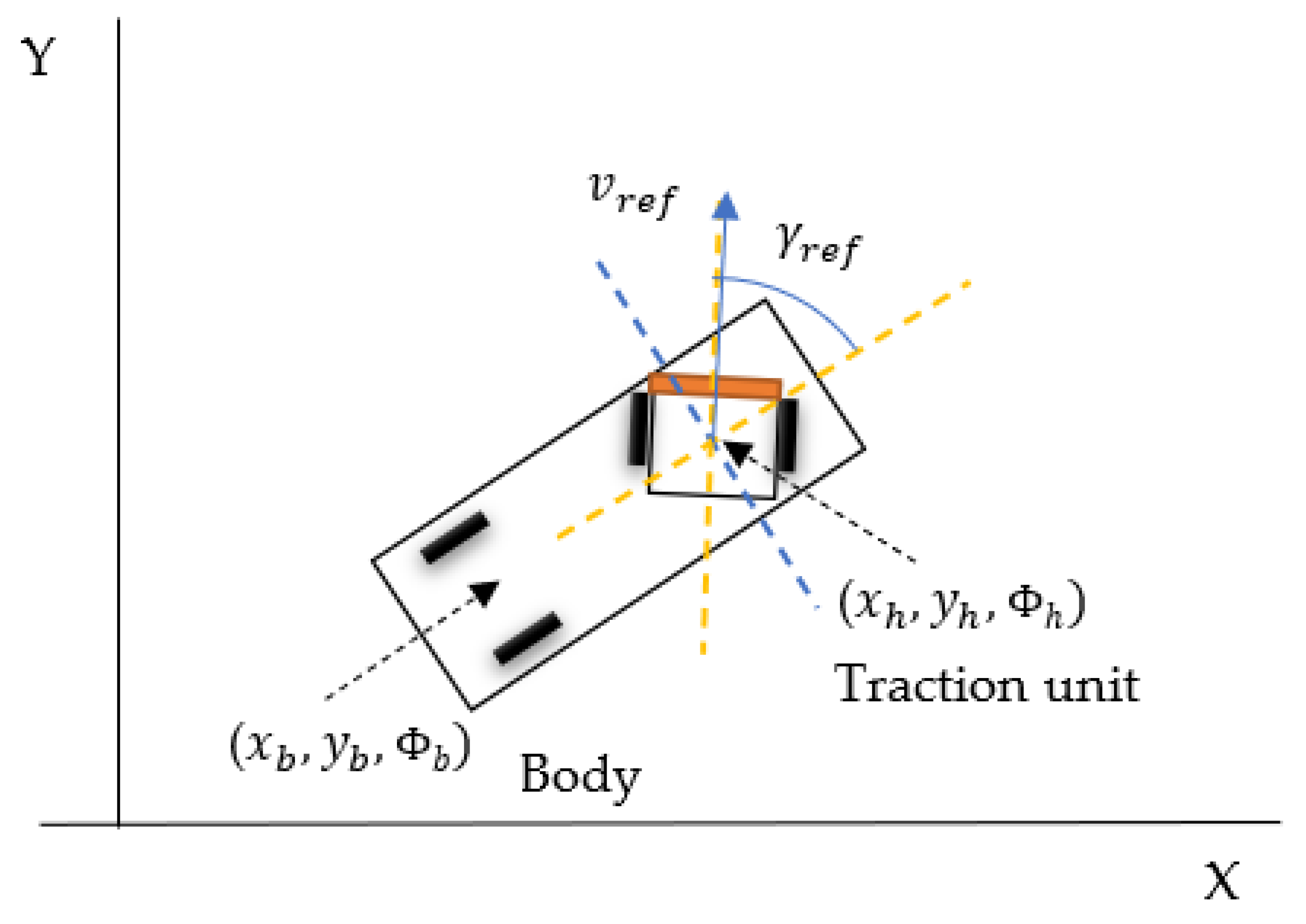
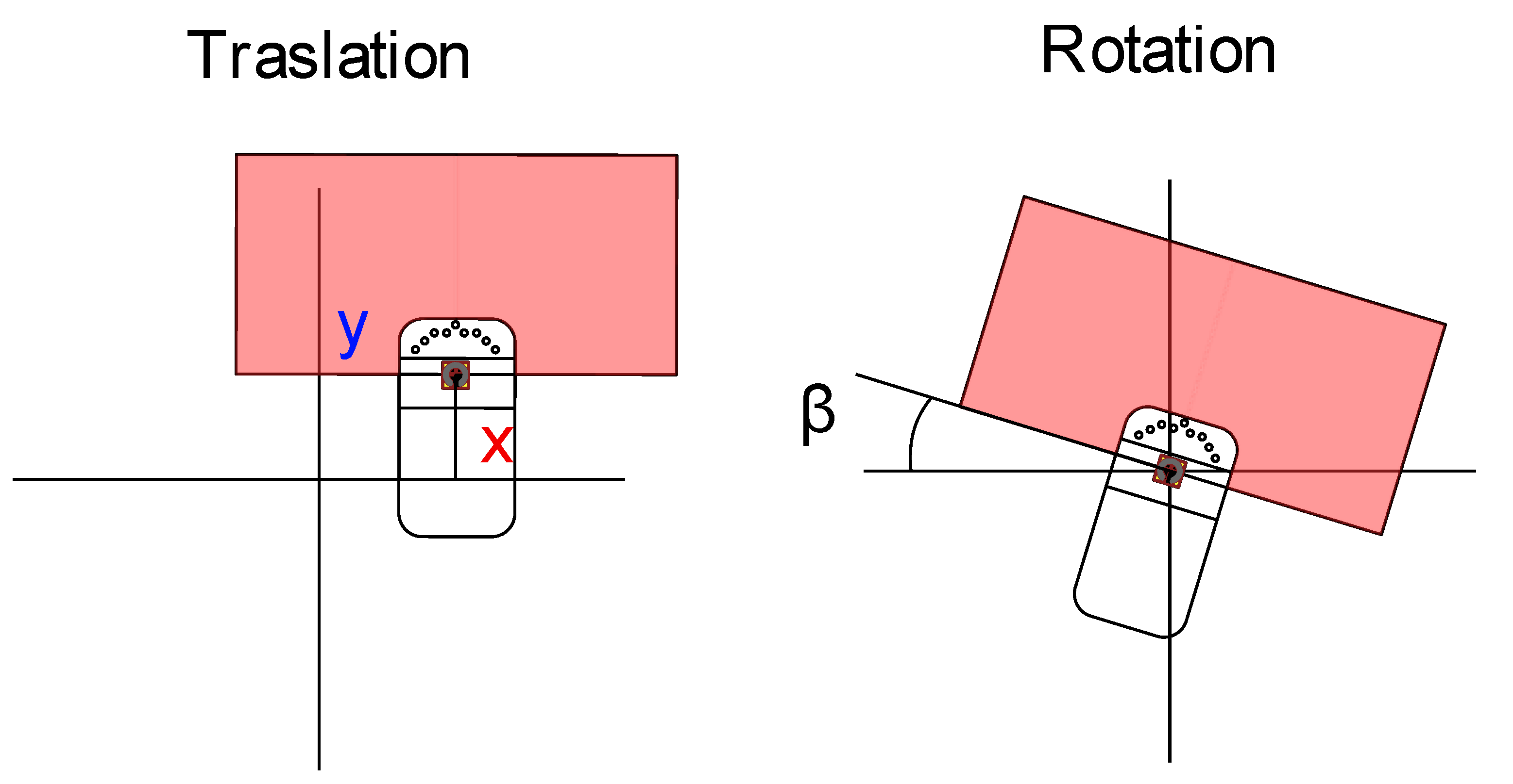
5.3.1. Position

When generating a trajectory, the first point to be considered is the coordinate system in which it is located. In this application, we work with two coordinate systems simultaneously: a general coordinate system called absolute, S 0 , and a relative coordinate system that will vary with the movement of the AGV, S R . both in Cartesian coordinates, although polar coordinates are also used for certain operations.
The UAM-05LP safety lidar measures distances and transmits these data in a format similar to polar coordinates, but instead of providing the angle in radians, the device indicates the sample number i of the lidar sweep. Knowing from the specifications that the UAM lidar takes 1080 samples per sweep and that its reading range is 270°, it is possible to convert it to polar coordinates (Equation (12)):
k s = 270 ° 1080   s a m p l e s = 0.25 ° / s a m p l e = 0.0043   r a d / s a m p l e
α i = i · k s
Then, multiplying k s by the sample index i given by the lidar, it is possible to obtain the angle α i associated with the sample i , and thus the polar coordinates d i , α i . Now, we need to transform them from polar to Cartesian using the simple expressions in Equations (14) and (15):
x i = d i · cos α
y i = d i · s e n α
where d i is the distance obtained by the laser at sample i , and x ,   y are the already transformed Cartesian coordinates. With these coordinates, every point p i detected by the lidar is located in the relative system S R . However, to get the position in the absolute coordinate system S 0 , it is necessary to perform one more transformation.
In Figure 11, we can see how the relative coordinate system S R , in red, moves with the AGV, and it is different from S 0 . Indeed, we must transform the points in S R detected by the lidar to the absolute coordinate system S 0 .
This transformation between coordinate systems is done with the transformation matrix. Transformation matrices reflect the displacement and rotation of the coordinate system relative to the absolute.
Luckily, the coordinate system is two-dimensional because the laser performs two-dimensional sweeps without moving on the vertical axis. This simplifies the calculations by reducing the size of the matrix to 3 × 3, i.e., the rotation exclusively around the z-axis and the translations on the x-axis and y-axis.
For each degree of freedom (translation or rotation), there exists an equation that transforms the coordinates of the points measured in the relative system to the absolute system (Figure 12) given by Equation (16):
X = x + x ,   Y = y + y
And the rotation by Equation (17)
X = x s e n β + y c o s β ,               Y = x     c o s β y s e n β  
where X , Y denotes the coordinates of the point in S 0 , x , y is the location of S R in S 0 , x , y is the pair of coordinates of the point in S R , and β represents the angle of rotation.
This way, by combining the two individual movements, it is possible to use a vector approach to obtain the transformation matrix (Equation (18)).
T x , y , β = 1 0 X 0 1 Y 0 0 1 × cos β sin β 0 sin β cos β 0 0 0 1 = cos β sin β X sin β cos β Y 0 0 1  
p S 0 = T x , y , β × p S R  
Using Equation (18) any point detected in the relative coordinate system S R can be transformed into the absolute coordinate system, S 0 .
Once we know how to calculate the points to follow, we will need to generate the velocity and direction of the AGV to head toward them.

5.3.2. Reference of the Velocity

First, we estimate the speed at which the target moves, with two consecutive measurements separated by a certain cycle time Δ t . From these two measurements, the points P 1 and P 2 with relative coordinates P 1 = x t i 1 ,   y t i 1 , and P 2 = x t i ,   y t i , are obtained, where Δ t = t i t i 1 .
The distance between the consecutive points is:
d 12 t i = x t i x t i 1 2 + y t i y t i 1 2  
Once the distance has been calculated, the velocity of the objective V o b j is estimated by dividing the distance by the time elapsed between the measurements.
V m t i = s i g n x t i 2 + y t i 2 x t i 1 2 + y t i 1 2 d 12 t i Δ t  
V o b j t i = V A G V t i 1 + V m t i
It is also necessary to consider if the objective approaches or moves away from the AGV. To do it, we have included the sign function in Equation (19) that in case of approaching V o b j it will be negative, and if moving away, it will be positive. To follow the objective, we generate a reference for the angular speed and a reference for the longitudinal speed. The reference for the longitudinal speed considers the module of the velocity; therefore, at this moment, we do not pay too much attention to its direction.
This speed input will feed one of the inputs of the speed controller, which is in charge of calculating the speed of the AGV to reach the target. First, we estimate the necessary acceleration to reach the object. We assume that, for small intervals ( Δ t ), the AGV travels with uniform acceleration. The acceleration needed to reach the target speed in 1 s can be then obtained from the following kinematic formula:
a R E F t i = V o b j 2 t i V A G V 2 t i 1 2 x t i 1 2 + y t i 1 2  
From this reference of acceleration, it is possible to calculate the speed reference (Equation (24)).
V r e f t i = V A G V t i 1 + a R E F t i Δ t

5.3.3. Reference for the Direction

Now, to obtain the direction, we use the mathematical basis of the Pure Pursuit path-tracking algorithm that calculates the trajectories using circumference arcs between the current point and the next one. The idea behind this algorithm is inspired by the way humans drive vehicles to follow a road, that is, looking ahead and changing the steering of the vehicle to keep this point in the middle of the lane.
The algorithm starts from a “looking ahead” distance, l a h , which is the next point on the path to follow. The look-ahead distance affects the tracking behavior. A large look-ahead distance imposes a large distance to the tracking target. To work closely with the human worker, it would be better to have a small value. However, very small values may create oscillations around the trajectory.
To reach the next point of the trajectory, the program will calculate the radius of the arc that links the current position of the vehicle with the next point.
Figure 13 shows a schematic representation of the pure pursuit algorithm. The next point to be reached has coordinates x ,   y , and we must find the radius r of the circumference arc that links the points x ,   y and x R ,   y R . The origin of this circumference is the instantaneous center of rotation (ICR), which is located at a distance r = x + d x from the point x R ,   y R .
From Figure 13, it is possible to deduce:
y 2 + x 2 = l a h 2  
d x = r x  
r x 2 + y 2 = r 2  
By manipulating Equation (27) and substituting Equation (25), it is possible to obtain the turning radius:
r = l a h 2 2 x = l a h 2 sin α
In this vehicle, considering the kinematic constraints, the steering angle γ is given by the relationship between the distance from the front and rear wheels d w to the turning radius r . Therefore, from Equation (28) and considering the kinematic constrains, the steering angle is obtained.
γ R E F = atan d w r = atan 2 sin α d w l a h
It is important to set the value of the distance l a h correctly; if l a h is too small, the robot will try to pass very accurately through the given points; however, the curvatures will be very large and the robot could end up zigzagging, skidding, and even overturning if the speed is high. On the other hand, if l a h is too large, the robot will make little effort to follow the path; thus, it may deviate too much from the way points.
In a human-following application, it is not so important that the robot passes exactly through the points where the human has passed. It is preferable that the robot tracks the trajectory of the human with smooth and predictable paths. From this perspective, it is better to manage medium-large look-ahead distances to avoid oscillations.
However, too large look-ahead distances can limit human–robot collaboration. Some specific collaborative tasks, such as synesthetic teaching, demand very small distances as the robot must follow the human very closely. However, other collaborative tasks, such as in logistic applications, do not require so small tracking distances. In the latter cases, the human can work closely with the robot to place or pick assets on/from the robot; meanwhile, the robot can stay immobile at the same location. Then, when the worker goes to the next location to perform the picking or dropping operation, the robot follows the human operator to perform the logistic operation.
Additionally, l a h is a configurable parameter of the algorithm, and it must be tuned by the user considering the requirements of the application: the workplace space limitations, the typical trajectories that the human will perform, the speed, the operation times, etc. All the variables and parameters that have been used to generate the control references are shown in Table 3.

6. Results and Discussion
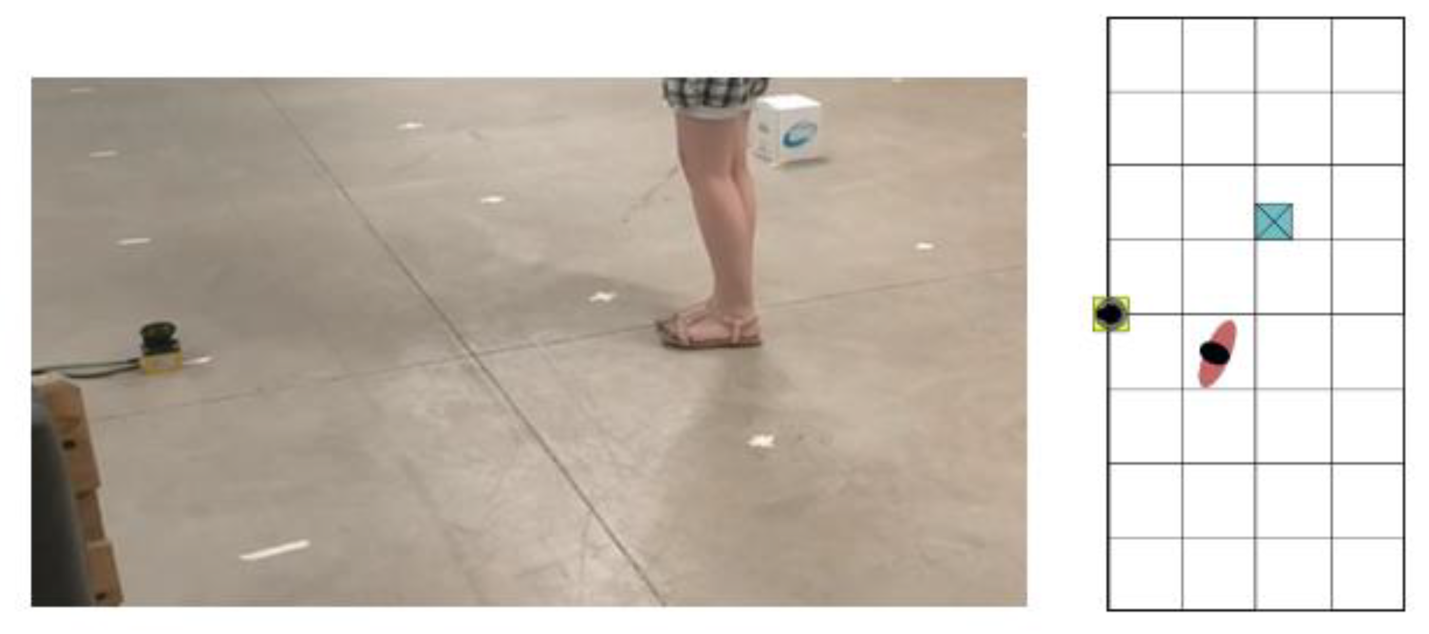
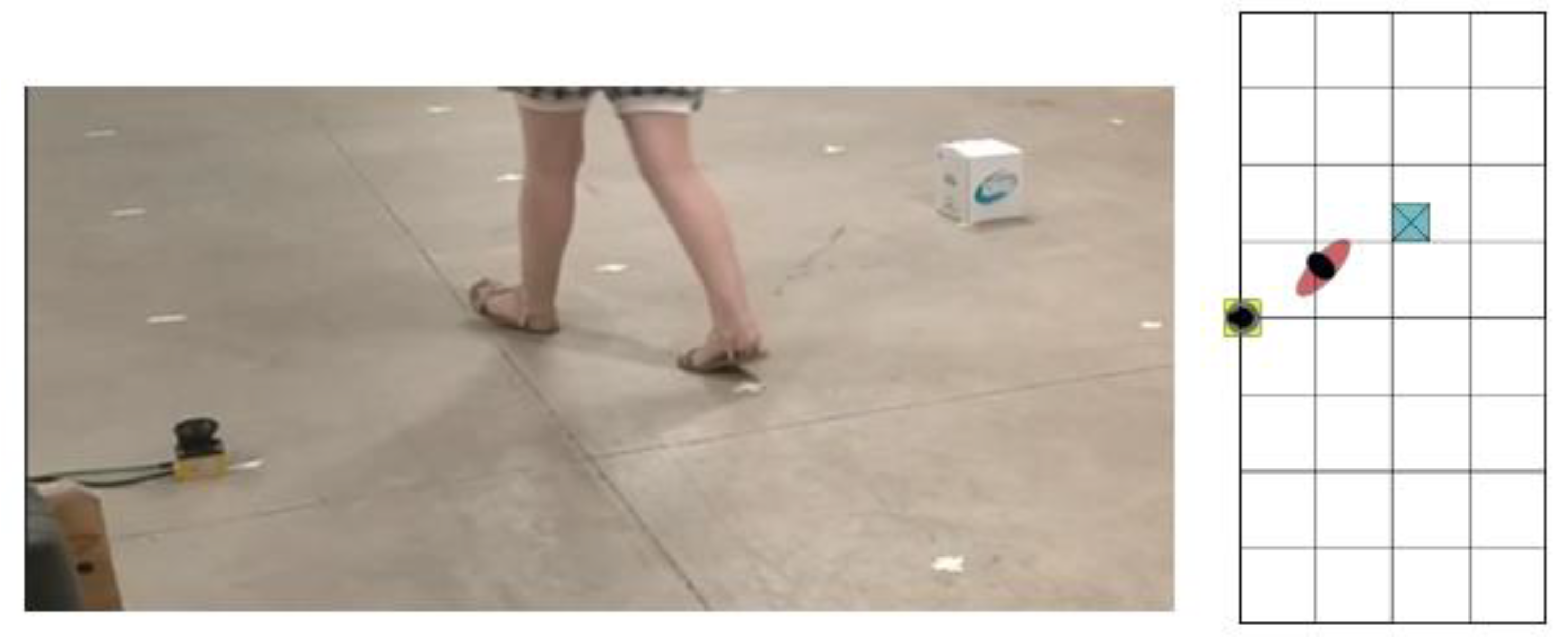
6.1. Static Tests

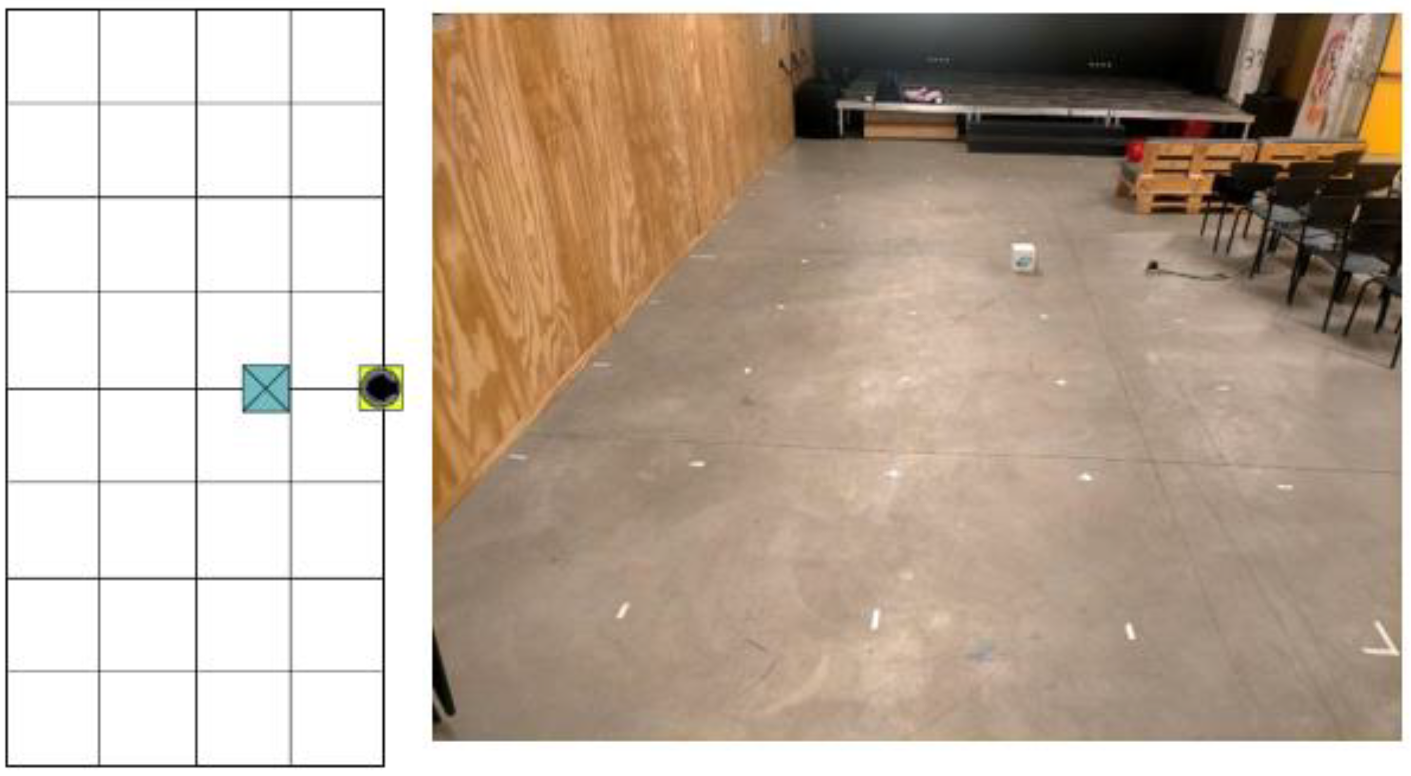
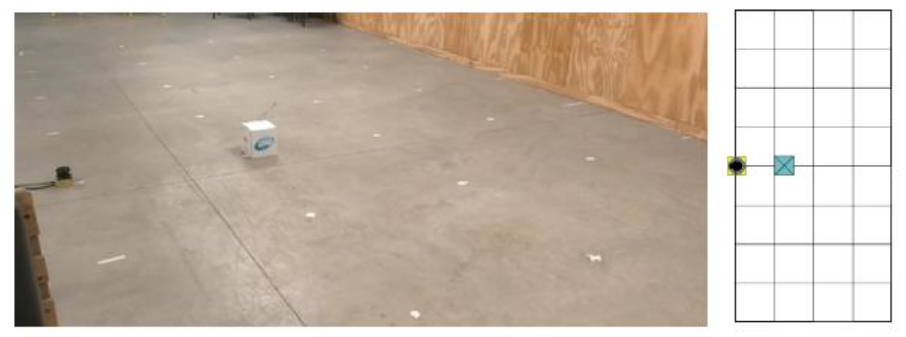
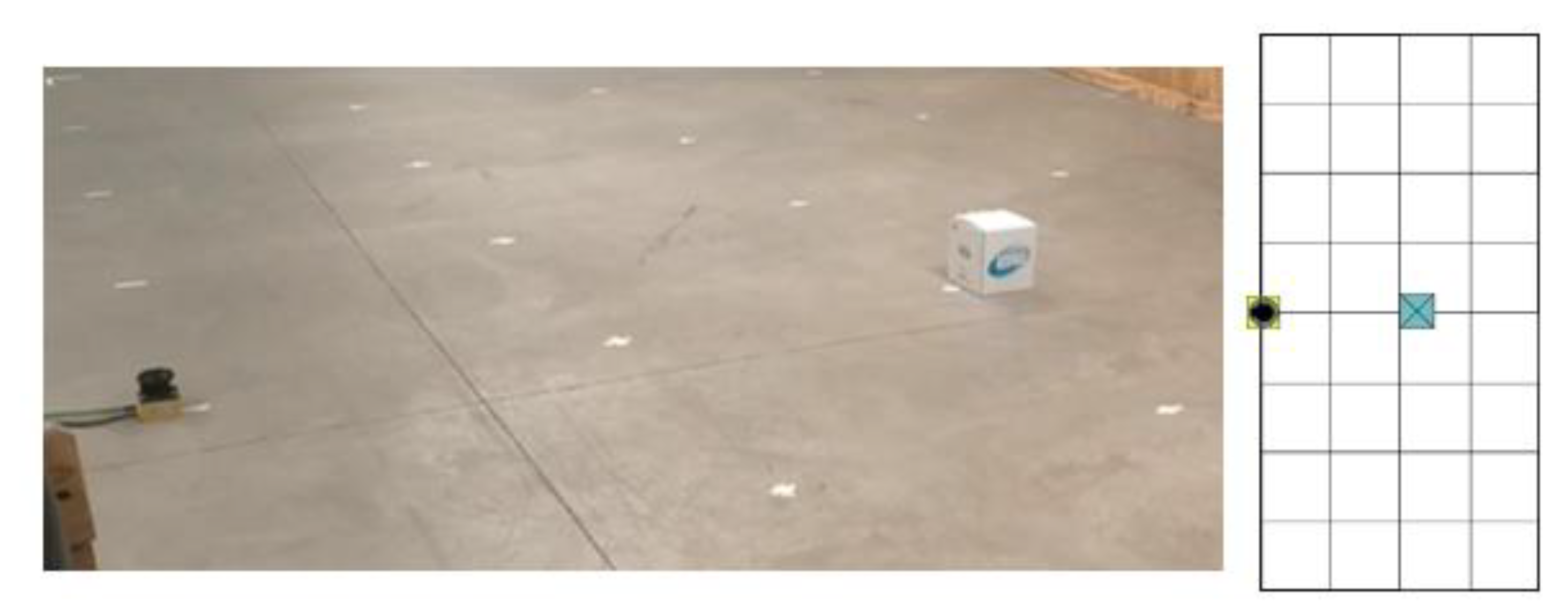
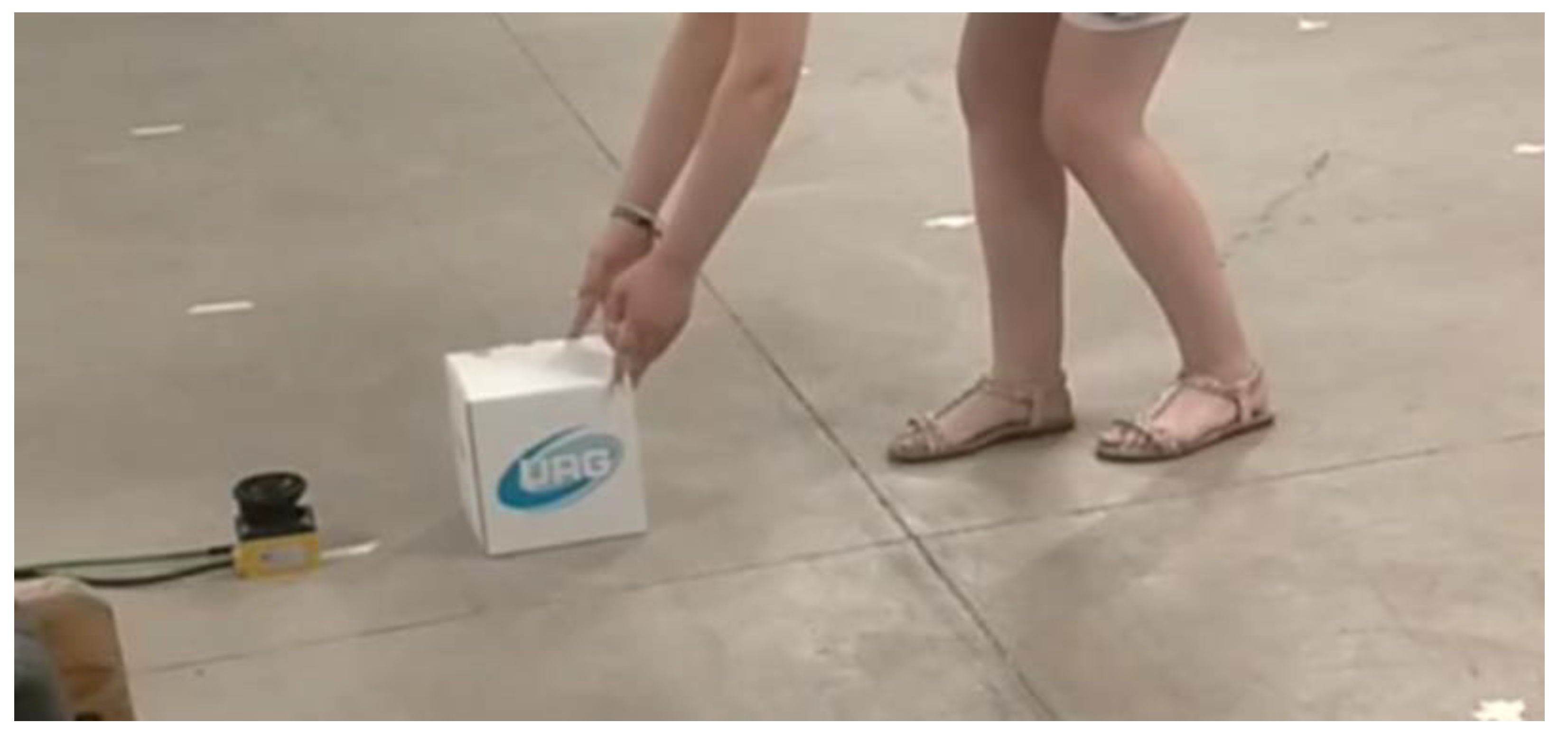
6.1.1. Setup of the Experimental Scenario

In the first test, the aim is to measure the accuracy with which the laser obtains distances, its ability to follow the target without losing it as far as possible and to check if it correctly detects the crossing of objects. To this end, we need a relatively large but controlled space, so outdoor tests are discarded to avoid wind, animals, or other disturbances.
To efficiently measure the actual distances accurately but without interfering with the measurements, a laboratory space of at most 4 × 8 m (detection range planned) is used. A grid of one-meter square cells is drawn carefully on the floor, marking the grid intersections to locate the exact meter points. Finally, as shown in Figure 13, the laser is placed on the first row and fourth column.
A camera on a tripod focusing on the grid is used to record the process. The experimental results will be compared with the ones generated by the following program. As the target, we used the laser box since it was easy to move and had enough size to be detected by the lidar (Figure 14).
Finally, it is worth it to note that to obtain an accurate measurement of the distances, the box was placed with the closest corner of the box coinciding with the cross marked on the floor. In the case of placing the box in the center, then the side of the box is on the grid line. This way, we ensured that the closest point coincides with the intersection points of the grid.

6.1.2. Description of the Tests

To check the quality of object detection, these were placed on the exact points of the grid, and the obtained real data were compared with those of the following program. For this first test, we moved the testing object in various directions and checked the position, velocity, and direction values obtained.
The second test assessed the ability to track a target once it is fixed and ignore other objects placed even at a shorter distance but without crossing.
Finally, in the third test, we evaluated the algorithm’s ability to detect the crossing of external objects. In addition, we checked whether the program continues after a momentary crossing or whether it stops when the crossing exceeds the safety time.
To illustrate these tests, in the following sub-sections, we show screenshots extracted from the videos recorded during the tests and a diagram showing the position of the target. We also show the data extracted from the recording during the measurement and screenshots of the information displayed on the screen by the program.

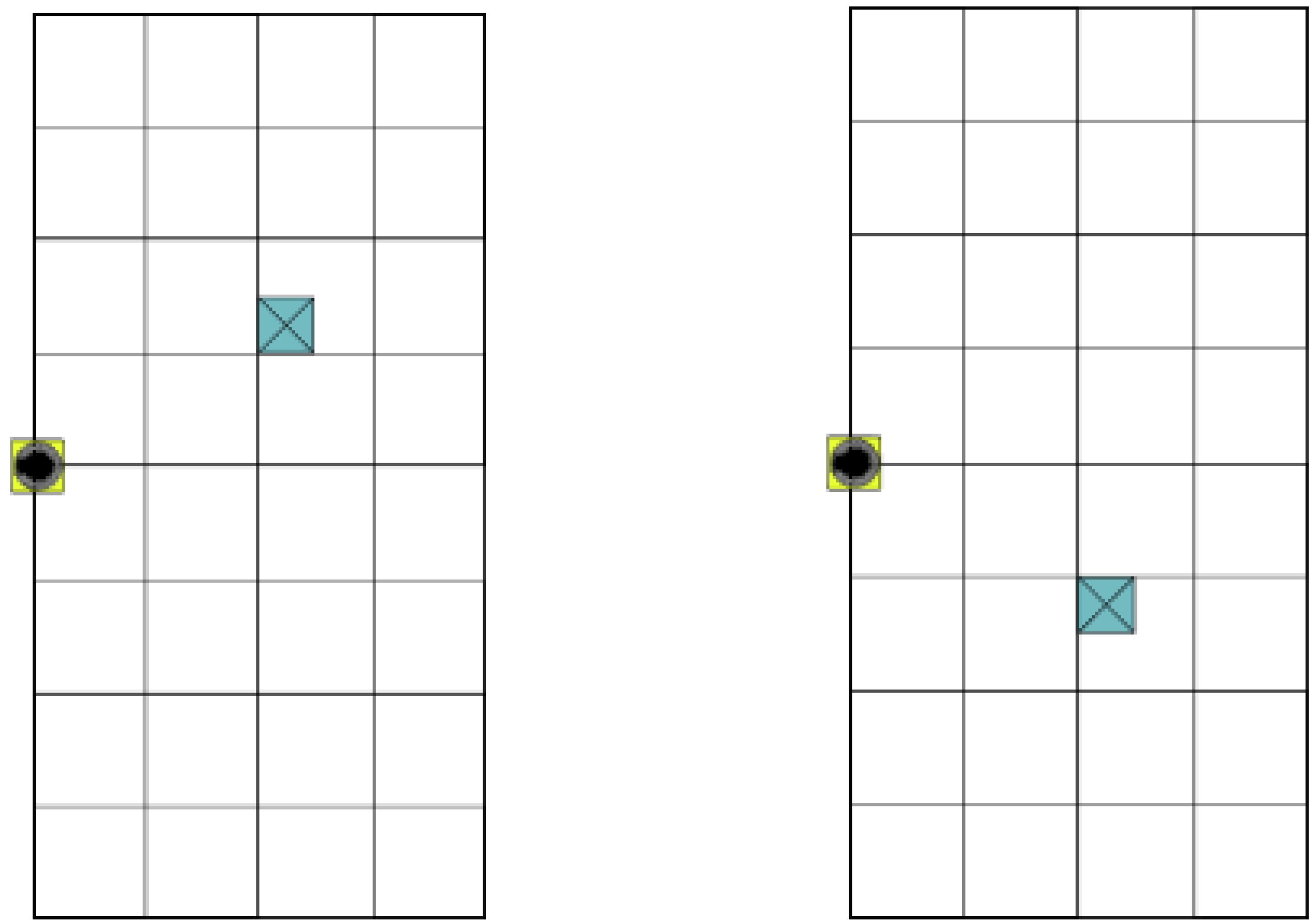
6.1.3. Position Test

We start by placing the object in position (0, 1), according to the coordinate system set by the grid, so that the laser can detect it as the object to be tracked (Figure 15). Once this is done, we start the execution of the program.
The data obtained at this instant showed that the closest object detected was at a position in the range X = [−0.05, 0] and Y = [0.93, 0.95]. This variation is due to the fact that the side of the box is parallel to the grid line, and at such a short distance, the laser detects all points of the side of the box closest to the lidar at a similar distance due to its accuracy. On the other hand, we observe a maximum variation of a couple of cm on the Y-axis. We attribute the 5 cm error with respect to the position to the inaccurate positioning of the box.
The log of the program shows the timestamp, the command sent to the AGV, and the target position detected by the lidar in cartesian coordinates. The command is sent in JSON format with three fields: “com”, “speed”, and “dir”. The field “com” indicates the action to be executed; “VEL” means that the action is to update the speed and direction references, and the variable “speed” stores the target speed; the field “dir” stores the target direction. The following lines are an example of the output of the program at the date/time indicated:
[28/06/2022 19:25:38]{“com”:”VEL”,”speed”:”0”,”dir”:”0”},
target position X: −0.04, Y: 0.93
[28/06/2022 19:25:39]{“com”:”VEL”,”speed”:”0”,”dir”:”0”},
target position X: −0.04, Y: 0.93
[28/06/2022 19:25:39]{“com”:”VEL”,”speed”:”0”,”dir”:”0”},
target position X: −0,05, Y: 0,94
Then we started to move the box backward to point (0, 2) (Figure 16).
The output of the program during this movement was:
[28/06/2022 19:25:46]{“com”:”VEL”,”speed”:”0,15”,”dir”:”0”},
target position X: −0.02, Y: 1.34.
[28/06/2022 19:25:46]{“com”:”VEL”,”speed”:”0,23”,”dir”:”0”},
target position X: −0.01, Y: 1.48
[28/06/2022 19:25:46]{“com”:”VEL”,”speed”:”0,37”,”dir”:”0”},
target position X: 0.02, Y: 1.64
[28/06/2022 19:25:47]{“com”:”VEL”,”speed”:”0,49”,”dir”:”0”},
target position X: 0.01, Y: 1.76
At this point, we can observe how not only does the position on the y-axis change but also the velocity sent to the AGV starts to increase.
Once the target is at point (0, 2), Figure 17, we can observe that the samples reflect a position in range X   [−0.05,−0.01] and Y   [2,−2.01]. The variation in the x-axis has decreased. In addition, the velocity stabilizes at 0.94 m/s.
Samples taken during these instants:
[28/06/2022 19:25:51]{“com”:”VEL”,”speed”:”0,94”,”dir”:”0”},
target position X: −0.01, Y: 2
[28/06/2022 19:25:51]{“com”:”VEL”,”speed”:”0,94”,”dir”:”0”},
target position X: −0,02, Y: 2,01
[28/06/2022 19:25:52]{“com”:”VEL”,”speed”:”0,94”,”dir”:”0”},
target position X: −0,04, Y: 2,01
Finally, we moved the box first to the left and then to the right to check the correct measurement on the x-axis. When the box was moved to the left (Figure 18left), we obtained a position in the range X [−0.99,−1.02] and Y   [2.02, 2.03]. The velocity remained stable, but the direction varied until it stabilized between −0.41 and −0.42 rad (24–25°).
When the box was moved to the right (Figure 18right), we obtained a position of X   [−0.99, −1] and Y   [2, 2.01]. In this case, the speed increased to 1 m/s which is the maximum, and the direction stabilized between 0.41 and 0.42 rad.
The following lines show the output of the program when the target was in position (−1, 2):
[28/06/2022 19:26:22]{“com”:”VEL”,”speed”:”0,94”,”dir”:”−0,41”},
target position X: −0,99, Y: 2,03
[28/06/2022 19:26:22]{“com”:”VEL”,”speed”:”0,94”,”dir”:”−0,41”},
target position X: −1, Y: 2.03
[28/06/2022 19:26:23]{“com”:”VEL”,”speed”:”0,94”,”dir”:”−0,42”},
target position X: −0,99, Y: 2,02
And with the target at (1, 2):
[28/06/2022 19:26:22]{“com”:”VEL”,”speed”:”0,94”,”dir”:”−0,41”},
target position X: −0,99, Y: 2,03
[28/06/2022 19:26:22]{“com”:”VEL”,”speed”:”0,94”,”dir”:”−0,41”},
target position X: −1, Y: 2.03
[28/06/2022 19:26:23]{“com”:”VEL”,”speed”:”0,94”,”dir”:”−0,42”},
target position X: −0,99, Y: 2,02
To finish the position tests, we bring the object along the y-axis closer to a distance of less than 1 m (Figure 19). We observed how as soon as the object gets nearer than 2 m, the velocity drops rapidly towards 0.
The following lines show the output of the program during this test:
target position X: −0.01, Y: 1.04
[28/06/2022 19:27:05]{“com”:”VEL”,”speed”:”0”,”dir”:”0”},
target position X: 0.02, Y: 0.95
[28/06/2022 19:27:05]{“com”:”VEL”,”speed”:”0”,”dir”:”0”},
target position X: −0.05, Y: 0.84
[28/06/2022 19:27:05]{“com”:”VEL”,”speed”:”0”,”dir”:”0”},
target position X: −0.02, Y: 0.79
In addition to these tests, we have carried out other controlled experiments with the LIDAR placed at different positions. The resulting measures are shown in Table 4, Table 5 and Table 6 for the different laser positions (first column). As it is possible to see in Table 4, the laser is at −0.5, −0.5 position with 30° rotation in the z-axis. The position of the target is shown in the column “Object position”. To define these static positions, we have considered the angles: 0°, −30°, 30°, −45°, and 45° at different distances from the LIDAR. The column “Estimated position” indicates the absolute coordinates with respect to the origin. This estimation was obtained with the LIDAR measurement and homogeneous transformation matrices. All data have been measured three times, and the values of the table are the average of the three measurements. The last column expresses the error of the estimation regarding the real value of the coordinates.
As it is possible to observe in these tables, the estimation error is very small. We have considered the general transformation matrix with the value of translation and rotation according to every case. Every measure has been done three times, and the average has been used. The measure of the real distance between the laser and the object has been done with a laser distance meter. The largest errors appear when the angle is rotated, which may be due to inaccuracies when the object is located at a determined angle.
To sum up, the obtained values in the experiment are highly reliable, and they confirm the accuracy of our calculations for different positions of the laser, the object, or even both.

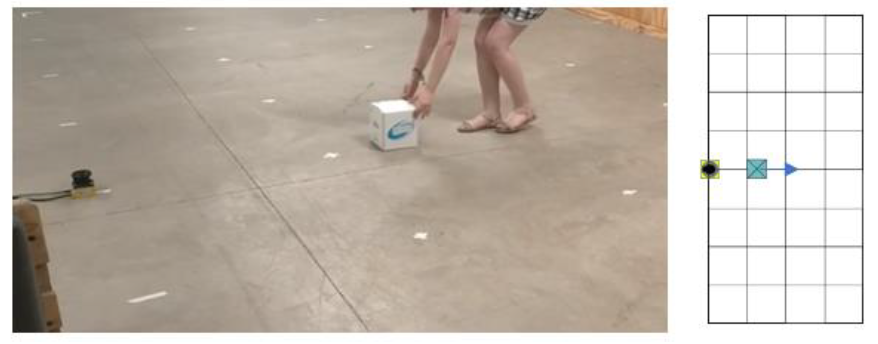
6.1.4. Tracking Test

To test the tracking, we placed the box at position (−1, 2), started the program, and checked that it was correctly detected during the target detection phase. Then, we asked the assistant to stand closer to the laser than the box (Figure 20), but without getting on the path, and we checked the output data.
The laser data still gave good values, X   [−0.99, −1.01] and Y   [2.02, 2.04]. This means that the detection cone worked successfully, and the assistant’s position was filtered, as expected.

6.1.5. Crossing Test

As a last validation during the static test campaign, we started with the laser detecting the target at position (−1, 2) and asked the assistant to step between the laser and the target. First, we performed a fast crossing in which the assistant passed without stopping in front of the target. After this, a crossing test was carried out in which the assistant remained between the target and the laser.
Figure 21 shows the output of the program when the object temporarily crosses, so the crossing lasts a very short time. It is possible to see how the system has detected the crossing during some samples; however, once the crossed object has passed, it detects the target again at the same position as before.
On the other hand, when the object crosses in front of the laser, and it remains for a period of time (Figure 22), the program detects it and outputs “tracking interrupted”. If this situation persists for a long time, the program is interrupted for safety reasons, and the operator must start the process again

6.1.6. Interpretation of Results
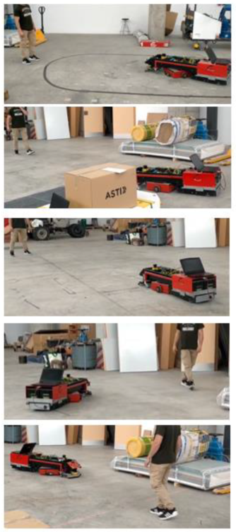
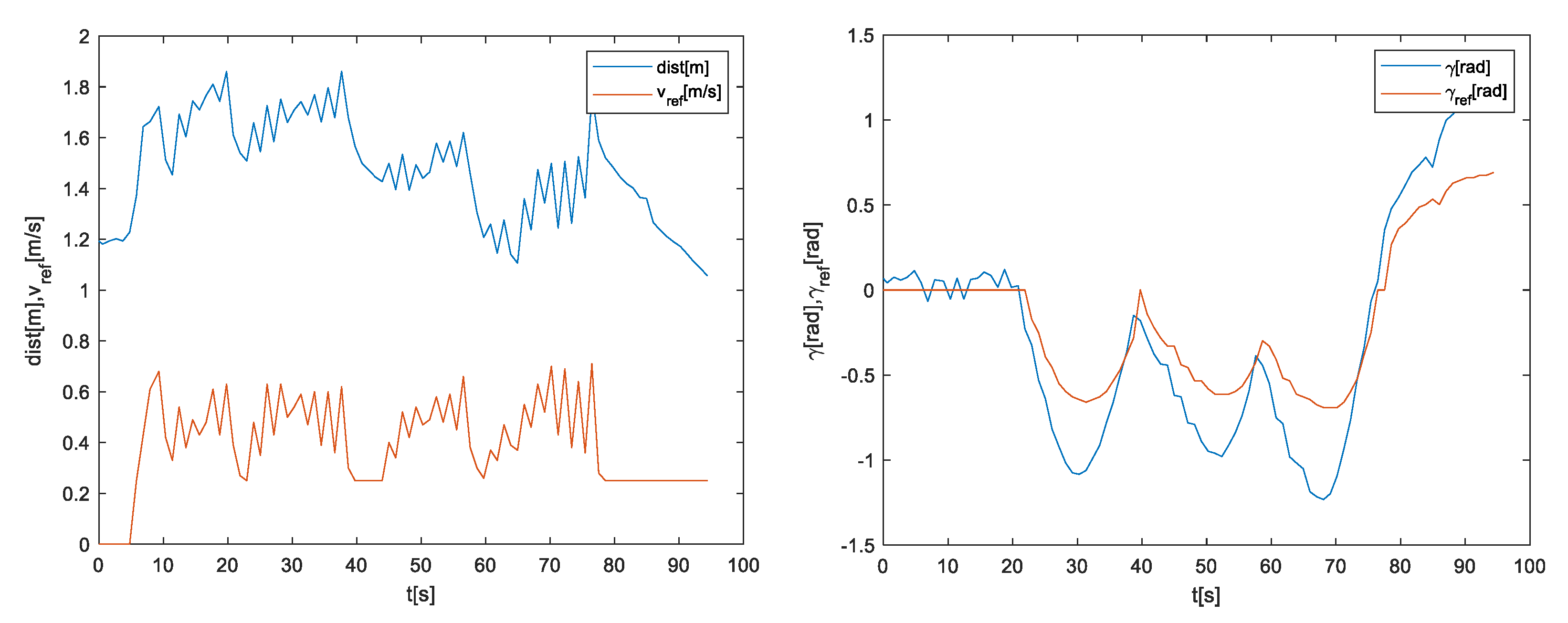
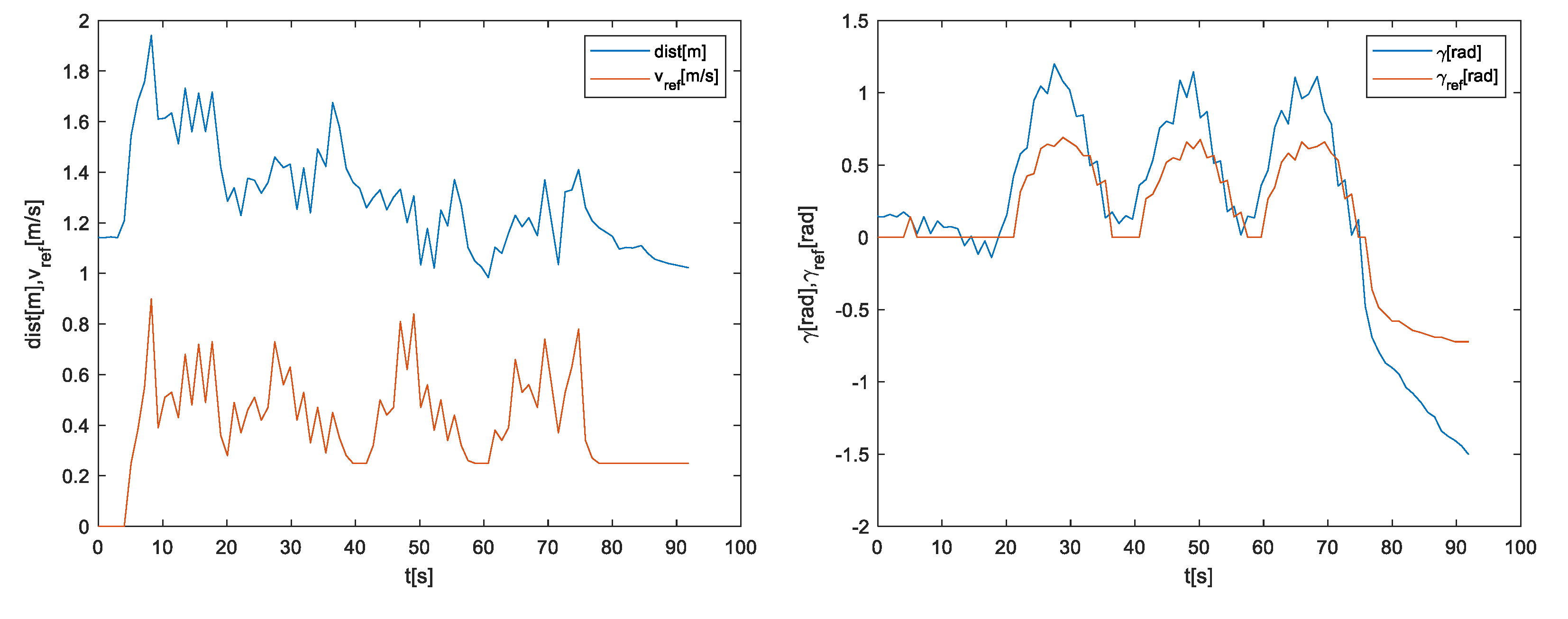
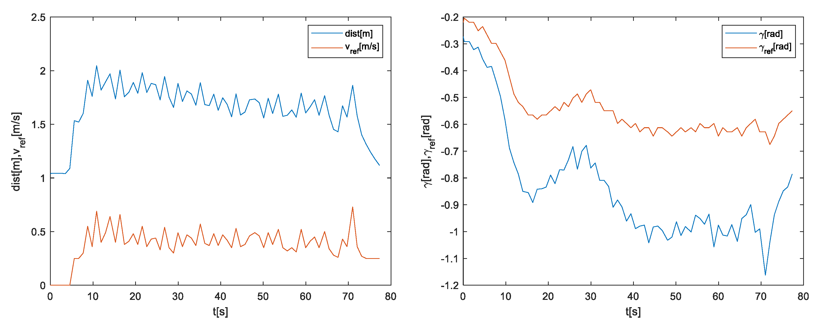
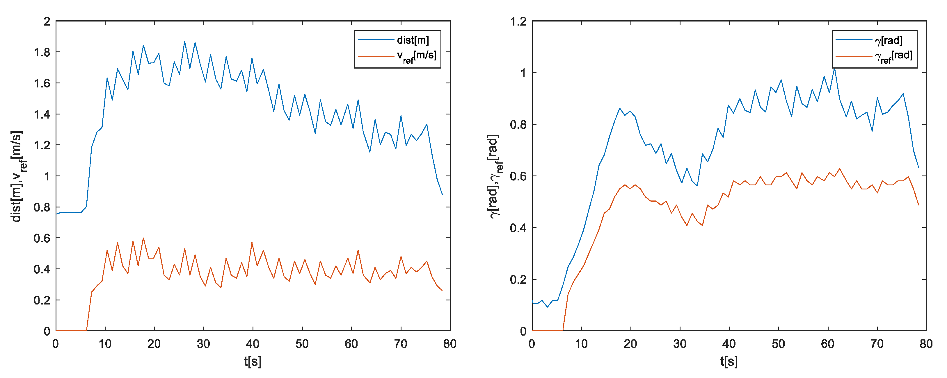
Based on the results of these tests, we can draw several conclusions. The calculation of coordinates and positions varies by an average of 2–3 cm during sampling, which can be considered an acceptable margin.
The accuracy and variation mentioned above vary very slightly, with the distance decreasing as we move away from the laser. This may be due to the fact that the number of samples of the object considered in a range of distances close to the lidar is greater than those taken at a farther distance. This results in a greater likelihood of obtaining very similar distances of the same object at different positions.
Once the object is moved to a more distant position, the velocity remains stable. This can be explained because the program believes it has already reached the velocity of the target, and therefore, the two systems maintain a constant distance.
The direction varies correctly with respect to the movements on the x-axis and remains at 0 when the object is kept on the y-axis, so it understands that it is in front of it.
The angle obtained (24°) is slightly less than the angle formed by the distance to the target and the y-axis (~26.5°). If we validate this data with the equation to calculate γ R E F we observe that the result is correct, considering a look-ahead distance of 1 m and a distance between front and rear wheels of 0.5 m.
γ R E F = atan 2 sin α d w l a h = atan 2 0.5 s e n 26.5 ° 1 24.04 °
We observed that the program is able to focus on the object it is tracking, ignoring other objects closer to the laser as long as they do not cross.
We also checked that the crossing detection works correctly, detecting the variation in the distance when an object is on the way. In addition, the program goes on running if the crossing is short and stops after the crossing safety time has elapsed.

6.2. Dynamic Tests

This test was performed in the AGVs laboratory of the University of Burgos, Spain. First, we connected a laptop where the following algorithm was running, the lidar and the AGV through an ethernet switch and a raspberry. Figure 23 shows the architecture for the dynamic tests. The raspberry was connected to the AGV by a CAN bus. The laptop sends UDP frames with the direction and speed references to the raspberry, and it translates them into CAN frames.
Figure 24 shows the location of these devices in the AGV.
To perform these tests, first, the connection between all elements was checked. Then, we sent control frames in an open loop with the AGV connected and observed how the speed and direction were modified by the messages sent. Once the communication with the AGV was verified, we proceeded to make the complete assembly, feeding the laser with a 24 V output of the AGV and connecting the laser, the computer, and the raspberry connected to the AGV using an ethernet switch.
The maximum speed was set to 0.5 m/s to easily control the AGV in case of failure and to protect the equipment and the computer on it.
Once the connection was checked and with that architecture, we realized that the AGV was moving in the right direction but twisting from one side to the other, trying to correct its direction to fit the target. To reduce this zigzag, we decided to increase the look-ahead distance from 0.5 m to 1 m, achieving a very substantial improvement in the smoothness of the turns.
Now, we obtained a successful dynamic test in which the AGV followed the target at low speed, correcting its heading to match that of the target but without extreme pitching. The AGV tracked the target forward and turned with it, reversing its direction.
Figure 25 shows a compilation of images that summarizes the execution of the dynamic test.

Performance Evaluation of the AGV with Different Trajectories

To complement the section of the experimental results, several experiments were carried out to follow a human describing different trajectories: a straight line, a square, and a circumference. Figure 26, Figure 27 and Figure 28 show the distance, the velocity reference, the angle to the target, and the direction reference for these trajectories. The figures on the left show the distance in blue and the velocity reference in red; the figures on the right show the angle to the target in blue and the direction reference in red.
Figure 26 and Figure 27 represent the results for the counterclockwise and clockwise square trajectories, respectively. In these figures, it is possible to observe that the velocity reference is related to the distance; if the distance grows, the velocity also does the same. Indeed, the peaks in the distance curve appear also in the velocity line. These peaks come from the steps of the human when walking. If the AGV followed a vehicle instead of a human, these peaks would decrease as the movement became more regular. The big jumps in the distance seem to match the edges of the square. At the beginning of the curve, the distance is maintained, so the speed reference is zero. When the target starts moving, the reference is updated in order to follow the target.
Another interesting result can be observed in the direction. It is possible to see how the direction reference has a similar shape to the trajectory described by the angle of the target but with a lower amplitude. This effect can be seen in both directions of movement. In this curve, there are three big peaks that match the first three edges of the square. In the counterclockwise square, the angles have a negative sign as the target is located on the left of the AGV. In the clockwise direction, the opposite happens; the angles and the reference are positive, as the target is located on the right of the AGV. In the beginning, the direction is zero because the AGV starts aligned with one of the segments of the square.
Figure 28 and Figure 29 represent the results for the counterclockwise and clockwise circular trajectories, respectively. The distance and velocity reference curves are similar to the square case but smoother. Although the same peaks appear due to the human-walking, the decreasing trend in the distance is more regular. It is also noticeable how the direction reference tracks the angle of the target. These curves are quite similar but with less absolute value. Unlike the square, the angle of the target does not present periodic peaks, as the circular trajectory is more regular. In addition, for both trajectories, the sign of the direction reference matches the direction of rotation: for clockwise is positive, and for counterclockwise is negative.
In addition to these graphical results, the performance of this approach has also been evaluated numerically, and the corresponding metrics are shown in Table 7. The minimum distance Dmin, maximum distance, Dmax, average distance, Davg, and the standard deviation of the distance Dstd, have been obtained.
For all these trajectories, the average distance is between 1 and 2 m, and the maximum distance is around 2 m. This result proves that the implementation of collaborative logistic applications with this system is feasible. As expected, the easiest movement to follow is the 0° straight line, and the hardest is circular.

7. Conclusions and Future Works

AGVs and autonomous robots are commonly used to replace conveyors and manual industrial trucks in the industrial sector. They commonly share their workspace with other vehicles and humans. Indeed, Industry 4.0 and its flexible production paradigm are promoting new human–AGV collaborative logistic use where humans perform complex tasks, and the robot transports parts or products. In this scenario, the person-following autonomous robot follows the operator to implement different logistic and industrial applications.
Hence, for this goal, we present in this work a control architecture and a control algorithm to implement human-following autonomous robots. Although any AGV or autonomous robot, regardless of kinematic setup, can use this approach, we used a tow AGV of ASTI Mobile Robotics to empirically validate this strategy, with a scanning laser UAM-05LT-301C as the sensor for real-time data acquisition.
The solution provides a high sensibility with a range of 2 to 5 cm, depending on the distance. It can perform 12 scans per second and track the desired target ignoring other elements within 30 cm of each other. Furthermore, it is able to detect a crossing element with a minimum detection difference of 30 cm. Static and dynamic test campaigns have been carried out to validate the proposal.
In future works, we can highlight the validation of the proposal with other different mobile robots, the adaption of the architecture to be used with different sensors, and the design of other filtering mechanisms.

Author Contributions

All authors contributed equally to the manuscript. All authors have read and agreed to the published version of the manuscript.

Funding

This research received no external funding.

Data Availability Statement

Data are available from the authors upon reasonable request.

Conflicts of Interest

The authors have no relevant financial or non-financial interest to disclose.

Abbreviations

AGVAutomated Guided Vehicle
CANController Area Network
ICRInstantaneous Center of Rotation
LIDARLight Detection and Ranging
PIDProportional Integral Derivative
RLCReinforcement Learning based Control
UDPUser Datagram Protocol (UDP)
UWBUltra Wide Band

References

  1. Echeto, J.; Santos, M.; Romana, M.G. Automated vehicles in swarm configuration: Simulation and analysis. Neurocomputing 2022, 501, 679–693. [Google Scholar] [CrossRef]
  2. Dintén, R.; López Martínez, P.; Zorrilla, M. Arquitectura de referencia para el diseño y desarrollo de aplicaciones para la Industria 4.0. Rev. Iberoam. Automática Inf. Ind. 2021, 18, 300–311. [Google Scholar] [CrossRef]
  3. Espinosa, F.; Santos, C.; Sierra-García, J.E. Transporte multi-AGV de una carga: Estado del arte y propuesta centralizada. Rev. Iberoam. Automática Inf. Ind. 2020, 18, 82–91. [Google Scholar] [CrossRef]
  4. Sierra-Garcia, J.E.; Santos, M. Combining reinforcement learning and conventional control to improve automatic guided vehicles tracking of complex trajectories. Expert Syst. 2022, e13076. [Google Scholar] [CrossRef]
  5. Wen, R.; Yuan, K.; Wang, Q.; Heng, S.; Li, Z. Force-guided high-precision grasping control of fragile and deformable objects using semg-based force prediction. IEEE Robot. Autom. Lett. 2020, 5, 2762–2769. [Google Scholar] [CrossRef]
  6. Sánchez, R.; Sierra-García, J.E.; Santos, M. Modelado de un AGV híbrido triciclo-diferencial. Rev. Iberoam. Automática Inf. Ind. 2022, 19, 84–95. [Google Scholar] [CrossRef]
  7. Zamora-Cadenas, L.; Velez, I.; Sierra-Garcia, J.E. UWB-based safety system for autonomous guided vehicles without hardware on the infrastructure. IEEE Access 2021, 9, 96430–96443. [Google Scholar] [CrossRef]
  8. Sandberg, A.; Sands, T. Autonomous trajectory generation algorithms for spacecraft slew maneuvers. Aerospace 2022, 9, 135. [Google Scholar] [CrossRef]
  9. Raigoza, K.; Sands, T. Autonomous trajectory generation comparison for de-orbiting with multiple collision avoidance. Sensors 2022, 22, 7066. [Google Scholar] [CrossRef]
  10. Sands, T. Flattening the curve of flexible space robotics. Appl. Sci. 2022, 12, 2992. [Google Scholar] [CrossRef]
  11. Manikandan, S.; Kaliyaperumal, G.; Hakak, S.; Gadekallu, T.R. Curve-Aware Model Predictive Control (C-MPC) Trajectory Tracking for Automated Guided Vehicle (AGV) over On-Road, In-Door, and Agricultural-Land. Sustainability 2022, 14, 12021. [Google Scholar] [CrossRef]
  12. Islam, F.; Nabi, M.M.; Ball, J.E. Off-road detection analysis for autonomous ground vehicles: A review. Sensors 2022, 22, 8463. [Google Scholar] [CrossRef] [PubMed]
  13. Pires, M.; Couto, P.; Santos, A.; Filipe, V. Obstacle detection for autonomous guided vehicles through point cloud clustering using depth data. Machines 2022, 10, 332. [Google Scholar] [CrossRef]
  14. Zahid, M.N.O.; Hao, L.J. A Study on Obstacle Detection for IoT Based Automated Guided Vehicle (AGV). MEKATRONIKA 2022, 4, 30–41. [Google Scholar] [CrossRef]
  15. Islam, M.J.; Hong, J.; Sattar, J. Person-following by autonomous robots: A categorical overview. Int. J. Robot. Res. 2019, 38, 1581–1618. [Google Scholar] [CrossRef]
  16. Honig, S.S.; Oron-Gilad, T.; Zaichyk, H.; Sarne-Fleischmann, V.; Olatunji, S.; Edan, Y. Toward socially aware person-following robots. IEEE Trans. Cogn. Dev. Syst. 2018, 10, 936–954. [Google Scholar] [CrossRef]
  17. Boschi, A.; Salvetti, F.; Mazzia, V.; Chiaberge, M. A cost-effective person-following system for assistive unmanned vehicles with deep learning at the edge. Machines 2020, 8, 49. [Google Scholar] [CrossRef]
  18. Tari, J.; Danès, P. Person Following from a Nonholonomic Mobile Robot with Ultimately Bounded Tracking Error. IFAC-PapersOnLine 2020, 53, 9596–9601. [Google Scholar] [CrossRef]
  19. Qiao, Y.; Fu, Y.; Yuan, M. Communication-Control Co-Design in Wireless Networks: A Cloud Control AGV Example. IEEE Internet Things J. 2022, 10, 2346–2359. [Google Scholar] [CrossRef]
  20. Tarmizi, A.I.; Shukor, A.Z.; Sobran NM, M.; Jamaluddin, M.H. Latest trend in person following robot control algorithm: A review. J. Telecommun. Electron. Comput. Eng. (JTEC) 2017, 9, 169–174. [Google Scholar]
  21. Moshayedi, A.J.; Li, J.; Sina, N.; Chen, X.; Liao, L.; Gheisari, M.; Xie, X. Simulation and validation of optimized PID controller in AGV (automated guided vehicles) model using PSO and BAS algorithms. Comput. Intell. Neurosci. 2022, 2022, 7799654. [Google Scholar] [CrossRef]
  22. Reis, W.P.N.D.; Couto, G.E.; Junior, O.M. Automated guided vehicles position control: A systematic literature review. J. Intell. Manuf. 2022, 34, 1483–1545. [Google Scholar] [CrossRef]
  23. Montesdeoca, J.; Toibero, J.M.; Jordan, J.; Zell, A.; Carelli, R. Person-Following Controller with Socially Acceptable Robot Motion. Robot. Auton. Syst. 2022, 153, 104075. [Google Scholar] [CrossRef]
  24. Pucci, D.; Marchetti, L.; Morin, P. Nonlinear Control of Unicycle-Like Robots for Person Following. In Proceedings of the 2013 IEEE/RSJ International Conference on Intelligent Robots and Systems, Tokyo, Japan, 3–7 November 2013; pp. 3406–3411. [Google Scholar] [CrossRef]
  25. Leigh, A.; Pineau, J.; Olmedo, N.; Zhang, H. Person Tracking and Following with 2d Laser Scanners. In Proceedings of the 2015 IEEE International Conference on Robotics and Automation (ICRA), Seattle, WA, USA, 26–30 May 2015; IEEE: Piscataway, NJ, USA, 2015; pp. 726–733. [Google Scholar]
  26. Petrov, P.; Georgieva, V.; Kralov, I.; Nikolov, S. An Adaptive Mobile Robot Control for Autonomous Following in Front of a Person. In Proceedings of the 2021 12th National Conference with International Participation (ELECTRONICA), Sofia, Bulgaria, 27–28 May 2021; IEEE: Piscataway, NJ, USA, 2021; pp. 1–4. [Google Scholar]
  27. Oh-Hara, S.; Saito, K.; Fujimori, A. Person following control for a mobile robot based on color invariance corresponding to varying illumination. IAES Int. J. Robot. Autom. 2022, 11, 33. [Google Scholar] [CrossRef]
  28. Tarokh, M.; Merloti, P. Vision-based robotic person following under light variations and difficult walking maneuvers. J. Field Robot. 2010, 27, 387–398. [Google Scholar] [CrossRef]
  29. Shaker, S.; Saade, J.J.; Asmar, D. Fuzzy inference-based person-following robot. Int. J. Syst. Appl. Eng. Dev. 2008, 2, 29–34. [Google Scholar]
  30. Jia, S.; Wang, L.; Wang, S.; Bai, C. Fuzzy-Based Intelligent Control Strategy for a Person Following Robot. In Proceedings of the 2013 IEEE International Conference on Robotics and Biomimetics (ROBIO), Shenzhen, China, 12–14 December 2013; IEEE: Piscataway, NJ, USA, 2013; pp. 2408–2413. [Google Scholar]
  31. Wang, L.; Wu, J.; Li, X.; Wu, Z.; Zhu, L. Longitudinal control for person-following robots. J. Intell. Connect. Veh. 2022, 5, 88–98. [Google Scholar] [CrossRef]
  32. Kautsar, S.; Gumilang, M.A.; Widiawan, B.; Tholabi, H.; Ariscandra, F. Contactless control system design for automatic guide vehicle (agv) based on depth camera. Food Agric. Sci. Polije Proc. Ser. 2021, 3, 136–144. [Google Scholar]
  33. Sierra-García, J.E.; Santos, M. Mechatronic modelling of industrial AGVs: A complex system architecture. Complexity 2020, 2020, 6687816. [Google Scholar] [CrossRef]
  34. Sánchez-Martinez, R.; Sierra-García, J.E.; Santos, M. Performance and Extreme Conditions Analysis Based on Iterative Modelling Algorithm for Multi-Trailer AGVs. Mathematics 2022, 10, 4783. [Google Scholar] [CrossRef]
Figure 1. Schematic representation of the AGV. The traction unit works as a differential mobile robot and is linked to the body by an axle on which it pivots. Thus, the kinematics of the AGV body follows the movement of a tricycle robot.
Electronics 12 02077 g001
Figure 2. General hardware architecture. The LIDAR generates the point cloud that is sent to the embedded computer, which runs the person-following algorithm. The embedded computer sends the direction and velocity reference to the AGV.
Electronics 12 02077 g002
Figure 3. Software control architecture. The SW architecture is composed of spatial and temporal filtering, a pure pursuit algorithm that calculates the direction, and the speed controller that obtains the velocity reference. In addition, a safety brake is implemented to decelerate the AGV if an object is too close.
Electronics 12 02077 g003
Figure 4. Flowchart of the human-following algorithm. The left part of the flowchart is the target detection phase; when the user confirms the tracking target, the algorithm proceeds to the target tracking phase. The system remains in this phase as long as no object obstructs the LIDAR.
Electronics 12 02077 g004
Figure 5. Spatial filter applied during the target detection phase. The tracking cone during this phase measures 90°. On the sides of this tracking cone, the objects are considered obstacles.
Electronics 12 02077 g005
Figure 6. Diagram that relates the constraints of the angle of the field of vision and the safety clearance to the obstacles. The distance to the obstacles must be larger than the look-ahead distance.
Electronics 12 02077 g006
Figure 7. Change in the detection cone with the distance (left) and object disappearing between samples (right). When the distance grows, the probability that a target disappears between the samples also grows.
Electronics 12 02077 g007
Figure 8. Variation of the number of samples in the detection cone with the distance. When the distance is smaller than 1 m or larger than 4 m, the number of samples in the cone is kept constant. Between these values, the number of samples decreases.
Electronics 12 02077 g008
Figure 9. Tracking of the target when passing near obstacles. The tracking cone moves with the target. The width of the tracking cone measured in LIDAR samples is 2 n s . This tracking approach allows us to move near obstacles without considering them as tracking targets.
Electronics 12 02077 g009
Figure 10. Crossing detection. When an obstacle appears between the LIDAR and the target, the crossing detection is triggered. This happens if the difference between distances is larger than d c .
Electronics 12 02077 g010
Figure 11. Absolute and relative coordinate systems when the AGV is in the starting position (left) and in motion (right).
Electronics 12 02077 g011
Figure 12. Example of translation (left) and rotation (right), where X, Y is the position of the center of the LIDAR and β is the rotation of the LIDAR, both in the inertial frame.
Electronics 12 02077 g012
Figure 13. Pure pursuit algorithm schematic representation, where l a h is the look-ahead distance and d w is the distance between the rear wheels and the center of the traction unit. The pair ( x R , y R ) represents the center of the rear axle.
Electronics 12 02077 g013
Figure 14. Static test environment setup. The LIDAR is in a static location, placed on the floor without the AGV. The object to be detected is the box of the LIDAR. The LIDAR is represented by a yellow square and the object by a blue one.
Electronics 12 02077 g014
Figure 15. Position test, target detection phase. The object is located in front of the LIDAR at position (0, 1). The angle from the LIDAR to the object is 0°, and there are not any obstacles between the LIDAR and the object. The LIDAR is represented by a yellow square and the object by a blue one.
Electronics 12 02077 g015
Figure 16. Position test, moving the target to (0,2). The object is moved carefully from (0,1) to (0,2), avoiding obstructing the LIDAR. The LIDAR is represented by a yellow square and the object by a blue one.
Electronics 12 02077 g016
Figure 17. Position test, target at (0,2). The object is located in front of the LIDAR. The angle from the LIDAR to the object is 0°. There are not any obstacles between the LIDAR and the object. The LIDAR is represented by a yellow square and the object by a blue one.
Electronics 12 02077 g017
Figure 18. Position test, target at (−1, 2) (left) and at (1,2) (right). When the object is located on the left, the angle is negative, and when it is on the right, it is positive. The sign of the direction reference matches the sign of the angle to the target. The LIDAR is represented by a yellow square and the object by a blue one.
Electronics 12 02077 g018
Figure 19. Position test, moving the target closer to the lidar. The object is placed very close to the LIDAR, so the velocity drops rapidly toward 0.
Electronics 12 02077 g019
Figure 20. Tracking test. The target object is located at (−1, 2). The target object is correctly detected by the tracking cone. When an obstacle approximates the LIDAR at a closer distance, at (1,1), the LIDAR still correctly detects the desired target thanks to the tracking cone. The LIDAR is represented by a yellow square, the object by a blue one, and the person by a pink ellipse.
Electronics 12 02077 g020
Figure 21. Output of the program during the crossing test when the target does not remain in the way of the lidar. In the captured image the decimal point is indicated by a comma.
Electronics 12 02077 g021
Figure 22. Crossing test, target remains in front of the lidar. The target is located at (−1,2). An unexpected element crosses between the target and the LIDAR, and it is detected as a crossing object. The LIDAR is represented by a yellow square, the object by a blue one, and the person by a pink ellipse.
Electronics 12 02077 g022
Figure 23. Architecture of the dynamic tests. In the dynamic experiments, the person-following algorithm runs on a laptop. A raspberry translates the velocity and direction commands to the CANbus frames to be interpreted by the AGV. The LIDAR is connected to the laptop and to the raspberry by a switch.
Electronics 12 02077 g023
Figure 24. Location of components in the AGV for the dynamic tests (laptop, raspberry, LIDAR, and switch).
Electronics 12 02077 g024
Figure 25. Dynamic test. The system detects the human target and follows it correctly for short and medium distances. Images show the change in the direction and even a loop to change the orientation.
Electronics 12 02077 g025
Figure 26. Result obtained when the human follows a counterclockwise square trajectory. The figure on the left shows the distance in blue and the velocity reference in red. The figure on the right shows the angle to the target in blue and the direction reference in red. The direction is negative because the target is located on the left.
Electronics 12 02077 g026
Figure 27. Result obtained when the human follows a counterclockwise square trajectory. The figure on the left shows the distance in blue and the velocity reference in red. The figure on the right shows the angle to the target in blue and the direction reference in red. The direction is positive because the target is located on the right.
Electronics 12 02077 g027
Figure 28. Result obtained when the human follows a counterclockwise circular trajectory. The figure on the left shows the distance in blue and the velocity reference in red. The figure on the right shows the angle to the target in blue and the direction reference in red. The direction is negative because the target is located on the left.
Electronics 12 02077 g028
Figure 29. Result obtained when the human follows a counterclockwise circular trajectory. The figure on the left shows the distance in blue and the velocity reference in red. The figure on the right shows the angle to the target in blue and the direction reference in red. The direction is positive because the target is located on the right.
Electronics 12 02077 g029
Table 1. Parameters of the model.
x h ,   y h Position of the Traction Unit
x b ,   y b Position of the body of the AGV
Φ h Orientation of the traction unit in the intertial frame
Φ b Orientation of the body of the AGV in the intertial frame
γ Angle of the traction unit in the AGV reference frame
γ r e f Reference for the angle of the traction unit
V L Longitudinal velocity of the left wheel
V R Longitudinal velocity of the right wheel
v h Longitudinal velocity of the traction unit
L h Length of the traction unit
L b Distance between the rear wheels and the traction unit
( Kp w , Kd w , KI w ) Gains of the PID
v r e f Reference for the longitudinal velocity
v L R E F Reference for the velocity of the left wheel
v R R E F Reference for the velocity of the right wheel
Table 2. Variables and parameters used in target tracking.
s c Safety Clearance
α f o v Angle of the field of view
l a h Look-ahead distance
w b Half of the widht of the AGV
N s p s Total number of samples of the LIDAR
n s r Variation of the number of samples in the detection cone with the distance
s m i n LIDAR Sample of the closest point
d c Minimum distance to detect a crossing event
T c Maximum crossing time, if the crossing takes longer than Tc the tracking phase finishes
r o k Last distance to obstacle before the crossing event
c d Crossing detection, when it values 1 there is a crossing object
Table 3. Variables and parameters for the generation of control references.
a R E F Reference for the Acceleration
V r e f Reference for the velocity
γ R E F Reference for the direction
V o b j Estimation of the velocity of the tracking target
l a h Look-ahead distance
d w Distance between the rear wheels to the traction unit
Table 4. Static test measurements with laser located at (−0.5,−0.5,30).
Laser PositionObject PositionEstimated PositionError
X [m]Y [m]Angle [°]X [m]Y [m]X [m]Y [m]X [m]Y [m]
−0.5−0.530−0.131.530.150.890.15−0.12
−0.5−0.530−0.801.13−0.630.88−0.130.01
−0.5−0.530−0.810.89−0.750.68−0.05−0.03
−0.5−0.5300.111.680.440.90−0.060.03
−0.5−0.5300.341.670.620.78−0.080.07
−0.5−0.530−0.982.36−0.172.02−0.170.01
−0.5−0.530−1.601.62−1.071.70−0.07−0.04
−0.5−0.5300.022.680.851.81−0.150.08
−0.5−0.5300.442.661.211.59−0.200.17
Table 5. Static test measurement with laser located at (0.5,0.5,−30).
Laser PositionObject PositionEstimated PositionError
X [m]Y [m]Angle [°]X [m]Y [m]X [m]Y [m]X [m]Y [m]
0.50.5−30−0.170.72−0.011.04−0.010.03
0.50.5−30−0.670.86−0.510.91−0.010.04
0.50.5−30−0.870.90−0.710.840.000.14
0.50.5−300.580.630.691.330.190.17
0.50.5−300.230.240.580.82−0.130.11
0.50.5−300.291.59−0.052.02−0.050.00
0.50.5−30−0.671.81−0.981.740.020.00
Table 6. Static test measurement with laser located at (0,0,0).
Laser PositionObject PositionEstimated PositionErrors
X [m]Y [m]Angle [°]X [m]Y [m]X [m]Y [m]X [m]Y [m]
0000.031.000.031.000.03−0.01
000−0.420.90−0.420.900.08−0.04
000−0.640.78−0.640.780.060.07
0000.540.850.540.850.040.02
0000.680.760.680.76−0.030.05
0000.112.030.112.030.110.00
000−0.881.80−0.881.800.120.06
000−1.391.07−1.391.430.020.01
0001.071.681.071.680.070.03
0001.451.451.451.450.030.03
Table 7. Performance evaluation for different trajectories.
TrajectoryDmin [m]Dmax [m]Davg [m]Dstd [m]
Square clockwise0.98 1.94 1.29 0.21
Square counterclockwise1.05 1.86 1.46 0.21
Circular clockwise 0.75 1.87 1.41 0.30
Circular counterclockwise 1.03 2.04 1.63 0.25
Straigth line (0 deg) 0.80 1.58 1.16 0.21
Straigth line (30 deg) 1.04 2.06 1.60 0.27
Disclaimer/Publisher’s Note: The statements, opinions and data contained in all publications are solely those of the individual author(s) and contributor(s) and not of MDPI and/or the editor(s). MDPI and/or the editor(s) disclaim responsibility for any injury to people or property resulting from any ideas, methods, instructions or products referred to in the content.

