Grid-Forming Converter Overcurrent Limiting Strategy Based on Additional Current Loop

Abstract

Compared with current source converters, voltage source converters (grid-forming converters) have better frequency support capabilities, voltage support capabilities, and regulation performance, thus they have broad application prospects. However, the grid-forming (GFM) converter has insufficient current control ability, and it easily causes problems such as overcurrent issues when a fault occurs. Thus, this insufficiency is one of the most important challenges the GFM converter is faced with. Aiming to solve the problems mentioned above, this paper proposes a control method of a GFM converter achieved with a low-pass filter structure and an additional current loop. The additional current loop controls the dq-axis current components by acting on the outer loop to generate appropriate phase and voltage amplitude reference. The low-pass filter structure is used to solve the system frequency stability problem caused by the inclusion of the additional current loop. On the premise of ensuring that the system frequency meets the grid-connection requirements, the proposed strategy rapidly limits the output current within the allowable range and guarantees expected voltage source characteristics of the converter during the fault period. Finally, the effectiveness and superiority of the proposed control strategy are verified by MATLAB/Simulink simulations.

1. Introduction

Due to the growing needs of the development of energy strategy in the new era, building a new power system with new energy as the main body is an inevitable choice for China to achieve its goal of “dual carbon”. Most new energy equipment, such as wind power generators and photovoltaic cells, are connected to the grid through power electronic converters, and their grid-connected control methods can be divided into grid-following (GFL) and grid-forming (GFM) controls [1,2,3,4].

At present, GFL is a general technical means of grid-connected control of power electronic converters and uses a phase-locked loop to measure the phase of the grid voltage to achieve power regulation while connecting to the grid [5]. However, the control mode of GFL does not have the support and regulation of grid frequency and voltage [6], especially in transient cases. This lack of support and regulation is because the GFL performs as a current source and does not have the ability to support transient voltage.

It is generally accepted that GFM can actively control the frequency and voltage output of the converter, but GFM converters can cause large short-circuit currents during faults. Since the converter can only withstand 20~50% of the overcurrent [7,8], the large short-circuit current will cause the converter to be out of service due to device protection and may even cause serious equipment damage. Thus, for GFM converters, limiting the overcurrent rapidly has become one of the focuses of research.

At present, the overcurrent limiting strategies during short circuits of GFM converters mainly include current amplitude limiting [9,10,11], virtual impedance [12,13,14,15], and power reference changing [16,17]. Among them, current amplitude limiting does not have transient voltage support capability and needs to be synchronized through a phase-locked loop, which easily causes system oscillation instability in the case of a weak power grid [18,19]. The current limiting strategy based on virtual impedance changes the reference voltage according to the difference between the actual and set current values, which is equivalent to putting a power-consumption resistor in the line. According to the difference in the calculation methods of virtual impedance and current, the virtual impedance can be divided into linear virtual impedance [20,21] and nonlinear virtual impedance [22]. However, the calculation of virtual impedance relies on the voltage droop and loop parameters, and the accuracy of parameters cannot be guaranteed in actual operation. These limitations result in the current being inaccurately controlled. In addition, the virtual reactance will cause the short-circuit current to contain an attenuated DC component, which will affect the current control effect. Power reference changing cannot achieve accurate control of the current during the fault process, nor can it make full use of the converter overcurrent capability. Researchers [16] changed the rated power of the converter according to the degree of voltage dip and calculated the reactive and active power reference values based on the new power reference of the converter. On the one hand, the new power reference value does not make full use of the short-circuit capacity of the converter, thus the short-circuit current it provides is too conservative. On the other hand, the DC component at the beginning of the fault cannot be suppressed in time due to the slow response of the outer loop.

Aiming to solve the overcurrent problem of GFM converter in case of symmetrical faults, this paper proposes a current limiting strategy based on additional current loop combined with a low-pass filter structure. This strategy generates the phase and voltage amplitude that meet the current limiting requirements, through the additional current loop, and then suppresses the frequency fluctuation caused by the additional current loop through the low-pass filter structure. By this way, this strategy realizes the smooth control of active frequency during the fault. On the premise of ensuring that the system frequency meets the requirements, this control strategy makes full use of the short circuit capacity of the converter to achieve rapid control of current. At the same time, the voltage source characteristics of the converter during the fault period are maintained to provide stable voltage support for the system.

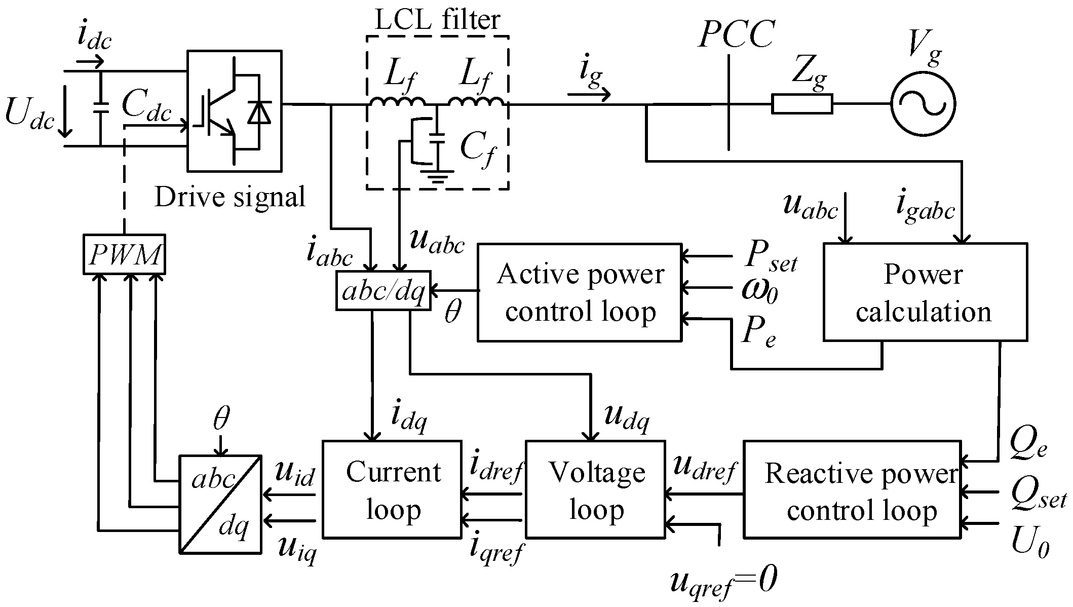
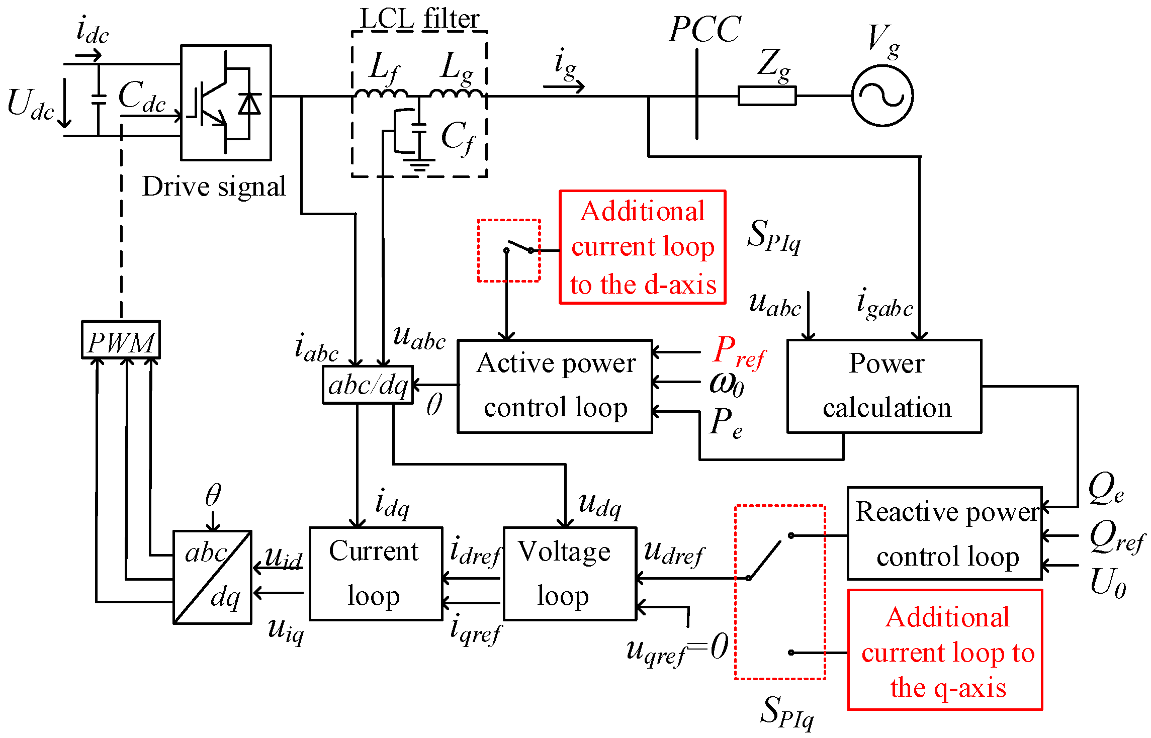
2. Proposed Current Limiting Strategy

The control structure of the GFM converter is shown in Figure 1.

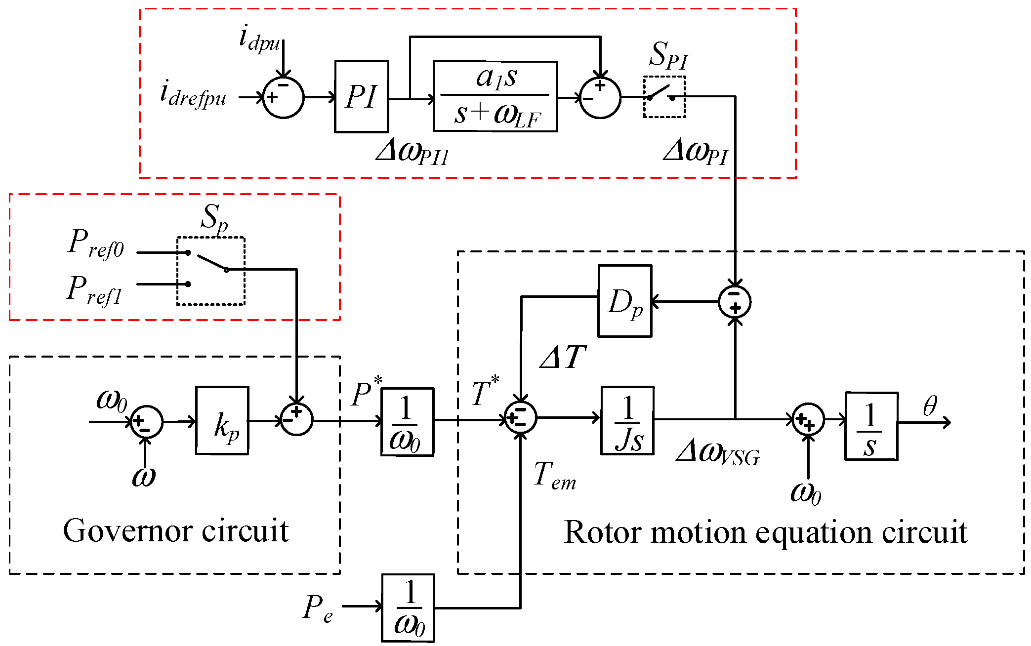
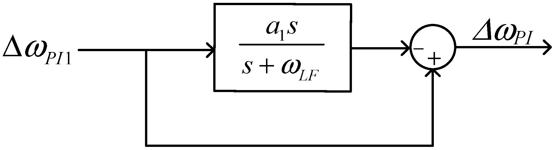
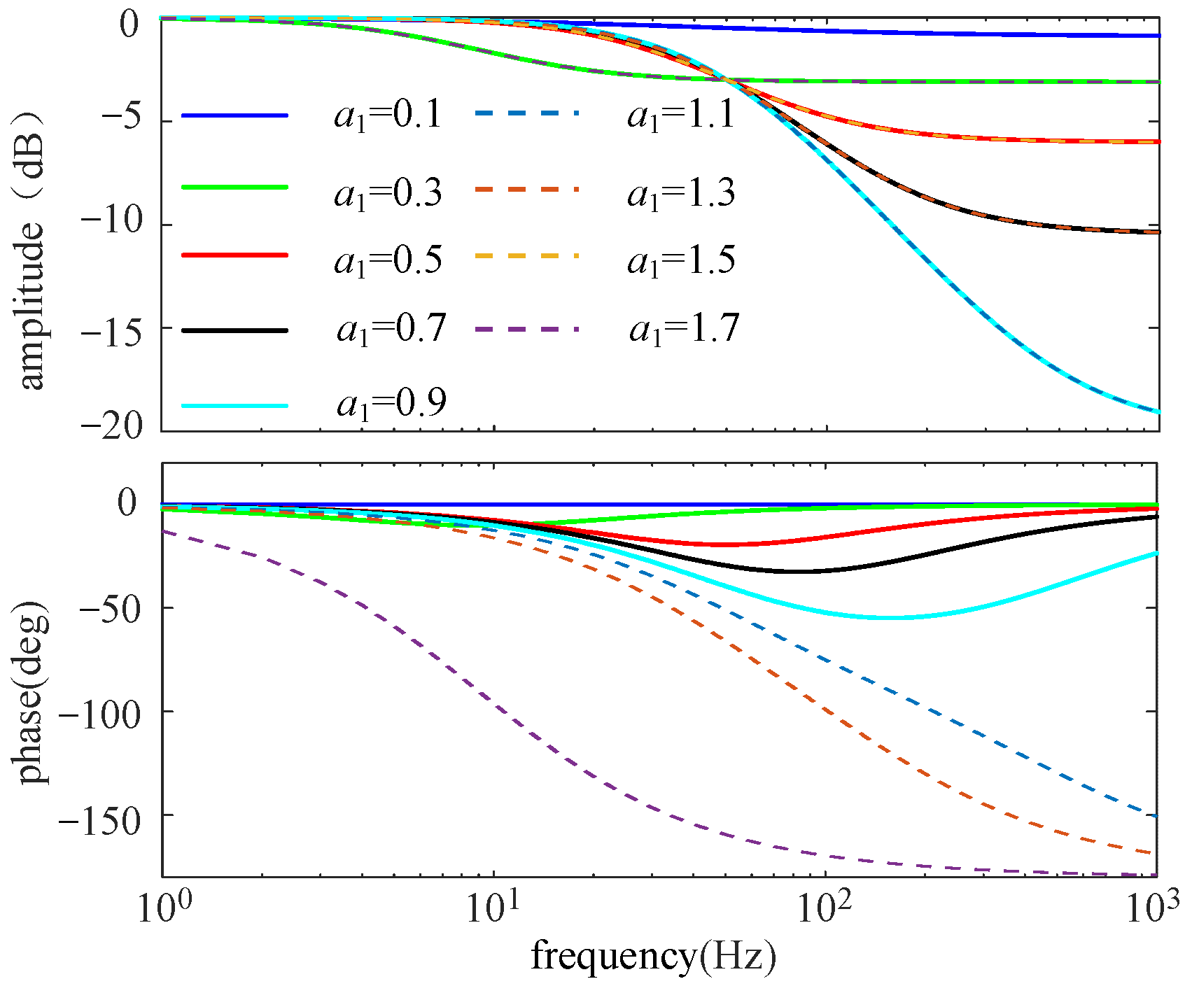
2.1. Active-Frequency Control Strategy

The virtual synchronous generator (VSG) control [23] is used for the active-frequency control link, and operating characteristics similar to synchronous generators are obtained by simulating the synchronous generator governor and rotor motion equation. This simulation can provide virtual inertia and synchronous power for the system.

During normal operation, the rotor equation of motion circuit in Figure 2 can be represented as,

$$J\frac{d^2\theta }{d{t}^2}=T^{*}-T_{em}-D_p(\omega -{\omega }_0)$$

(1)

where J represents the virtual inertia, T^* is the set value of the torque, T_em is the output torque, D_p represents the damping coefficient, and ω₀ is the reference angular velocity. T^* and T_em can be expressed as,

$$\left\{\begin{array}{l}{T}^{*}=\frac{P^{*}}{{\omega }_0}\\ T_{em}=\frac{P_e}{{\omega }_0}\end{array}\right.$$

(2)

where P^* is the reference value of active power generated by the virtual governor loop and can be calculated by the equation,

$$P^{*}=P_{ref}-k_p(\omega -{\omega }_0)$$

(3)

where k_p represents the active droop coefficient.

Substituting Equations (2) and (3) into Equation (1), we receive:

$$J\frac{d^2\theta }{d{t}^2}=T_0-T_{em}-D(\omega -{\omega }_0)$$

(4)

where T₀ = P_ref/ω₀, D = D_p + k_p/ω₀, and D represents the equivalent damping.

Due to the addition of the first-order inertial delay link, VSG equivalently increases the inertia and damping of the converter. Due to this increase, the converter has good anti-interference ability, which can suppress the peak value when the frequency fluctuates but will affect the power tracking speed [24]. Therefore, the control feature of VSG is conducive to system’s stability, but it is difficult for the converter to respond fast during the fault.

Therefore, an additional current loop is installed, and the active power reference is changed to improve the active’s response time during the fault. Figure 2 shows a control block diagram that takes the fault characteristics into account.

The additional current loop in the figure is used to reduce the damping, the active reference value is adjusted to be closer to the fault condition, and these two actions combine to accelerate the speed of the d-axis current control.

The active reference value is switched to Pref1 when a fault is detected and calculated from the d-axis current reference value during the fault as,

$$P_{\mathit{ref}1}=\frac{3}{2}{i}_{\mathit{dref}1}{u}_{\mathit{dref}}$$

(5)

where i_dref1 is the d-axis current reference and u_dref is the d-axis voltage reference during the fault.

As demonstrated in Figure 2, the output of the additional current loop acts to decrease the input of the D_P during the fault, which is equivalent to weakening the damping. Therefore, the active loop response is improved. When the d-axis current i_dpu is unstable, the output of the additional current loop is not 0, thus the damping is weakened. Additionally, when the current is controlled at the set value of i_drefpu, the additional current loop input is 0, the angular frequency is stable at ω₀, and the active power is stabilized at the given active reference of P_ref1, with ΔT = 0.

The switching of the active power reference and the input of the additional current loop will cause the output of the active control to jump, resulting in large frequency fluctuations. To address this problem, apart from the additional current loop, a low-pass filter (Figure 3) is added to suppress large fluctuations of frequency in the initial switching and eliminate frequency static errors. In Figure 3, Δω_PI1 represents the output signal of the additional current loop, and Δω_PI represents the output signal from the low-pass filter corresponding to Δω_PI1.

The transfer function of the filter link is,

$$G_{LF}\left(s\right)=\frac{\left(1-a_1\right)s+{\omega }_{LF}}{s+{\omega }_{LF}}$$

(6)

According to the reference frequency of the grid, the bandwidth of the low-pass filter is designed to be 75 Hz, and the gain amplitude of the filter at the cutoff frequency can be expressed as,

$$20{\log }_{10}\left|G_{LF}\left(s\right)\right|=-3$$

(7)

Substituting Equation (6) into (7), we receive:

$${\omega }_{LF}=150\pi \sqrt{\frac{{10}^{-0.3}-{\left(1-a_1\right)}^2}{1-{10}^{-0.3}}}$$

(8)

Figure 4 depicts the amplitude–frequency and phase–frequency characteristic curves for ω_LF as they alter with the value of a₁.

According to the amplitude–frequency characteristic curve analysis, the amplitude drop is evident when the low frequency band a₁ = 0.3 and 1.7, and the phase change is the smallest when a₁ = 0.3; thus, the filter parameters a₁ = 0.3 and ω_LF = 70.57 Hz are chosen.

2.2. Reactive-Voltage Control Strategy

The reactive power reference is the voltage loop control target during normal operation, and its control structure is illustrated in Figure 5. The d-axis voltage reference u_drefpu is generated through the integral controller and the voltage feed-forward link to adjust the reactive power Q_epu to the reference value Q_refpu [25,26]. The d-axis voltage reference can be calculated by the following formulae.

$$\Delta Q_{pu}=k_q\left(U_{0pu}-U_{pu}\right)$$

(9)

$$u_{drefpu}=\left(\frac{k_{qi}}{s}\right)(Q_{refpu}+\Delta Q_{pu}-Q_{epu})+U_{0pu}$$

(10)

$$u_{dref}=u_{drefpu}{U}_0$$

(11)

where ΔQ_pu is the reactive power regulation obtained by simulating the generator’s excitation; k_q and k_qi are the generator voltage regulation coefficient and integration coefficient of integral controller; U₀ is the voltage reference; and U_0pu, U_pu, and Q_refpu are the unitary value of reference voltage, filter capacitor voltage, and reference reactive power, respectively.

During a fault, the voltage loop control target in the proposed strategy changes to the q-axis current setting value i_qrefpu, which cannot be realized by the original control structure.

Therefore, switching to an additional current loop allows the GFM converters to maintain the voltage source characteristics and meet the voltage support requirements, as shown in Figure 5.

The additional current loop in Figure 5 is used to obtain a voltage reference matching the q-axis reference current. When a fault is detected, the switches S_q and S_PIq are closed, and the d-axis reference voltage can be calculated by the following equation.

$$u_{drefpu}=\left(k_{rp}+\frac{k_{ri}}{s}\right)(i_{qrefpu}-i_{qpu})+U_{0pu}$$

(12)

where k_rp and k_ri denote the proportion and integration coefficient of the additional current loop PI, respectively.

As illustrated in Figure 5, the system voltage is stable when the q-axis current stabilizes at the set value, and the additional current loop output stabilizes at a certain fixed value.

2.3. Selection of the dq-Axis Current Reference

According to China’s wind power grid-connected regulations [27], when grid voltage drops to 0.2~0.9U_N, the reactive current input must be 1.5(0.9 − U_s)I_N at least. Therefore, the dq-axis current reference during the fault can be expressed as follows.

$$i_{drefpu}=\left\{\begin{array}{l}{i}_{d0pu},\left(u_{pccpu}>0.9\right)\\ \sqrt{1^2-i_{qrefpu}^2},\left(0.2\le u_{pccpu}\le 0.9\right)\end{array}\right.$$

(13)

$$i_{qrefpu}=\left\{\begin{array}{l}0,\left(u_{pccpu}>0.9\right)\\ K_d\left(0.9-u_{pccpu}\right),\left(0.2\le u_{pccpu}\le 0.9\right)\end{array}\right.$$

(14)

where i_d0pu is the reference value of the d-axis current before the fault, K_d is the reactive current gain coefficient (generally not less than 1.5 because this paper adopts d-axis voltage orientation), and u_pccpu is the voltage amplitude of point of common coupling (PCC).

The improved control structure of the GFM converter is shown in Figure 6.

3. Simulation Results

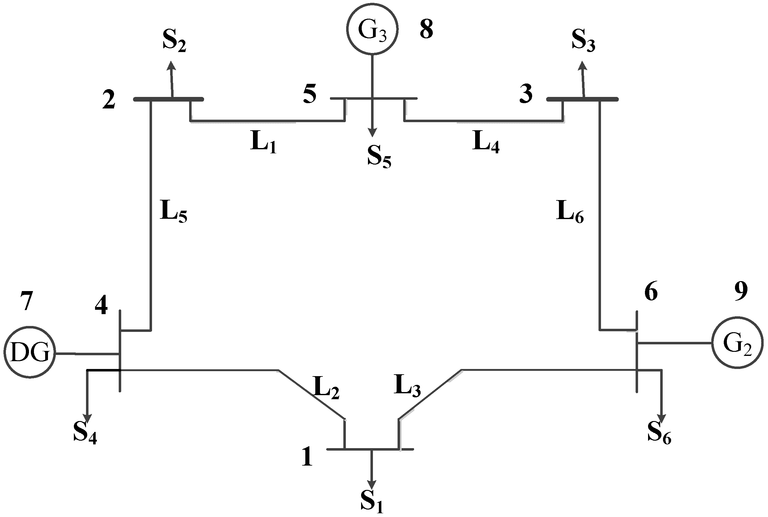
3.1. Test System Parameters

To test the performance of the proposed control strategy, a simulation was set up in Matlab/Simulink, and the corresponding system parameters are listed in

Table 1. Parameters of the simulated system.

Symbol/Unit	Quantity
f0/Hz	50
U0/V	380
Vdc/V	800
Lf/mH	1.5
Cf/uF	30
Lg/H	1
RL/Ω	0.3
LL/mH	0.4
Sn/kVA	15
Pref0/kW	15
Qref/kVar	0

. Power grid topology adopted in this paper can be seen in Appendix A. In this paper, a three-phase short circuit fault occurred in the system when t = 0.3 s, and the fault was removed when t = 0.7 s. The simulation duration was 1.2 s, and the overcurrent limit of the converter was set to 1.5 pu.

The following section will compare and analyze the overcurrent suppression effect and system characteristics of the converters under different control strategies.

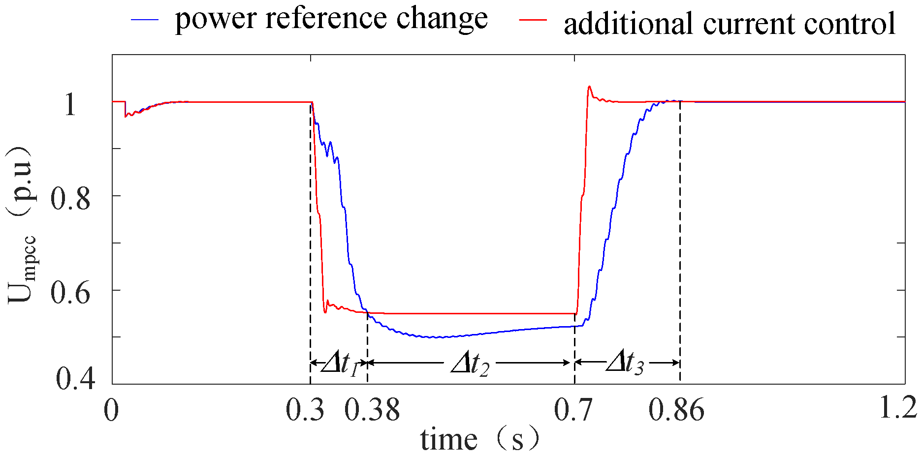
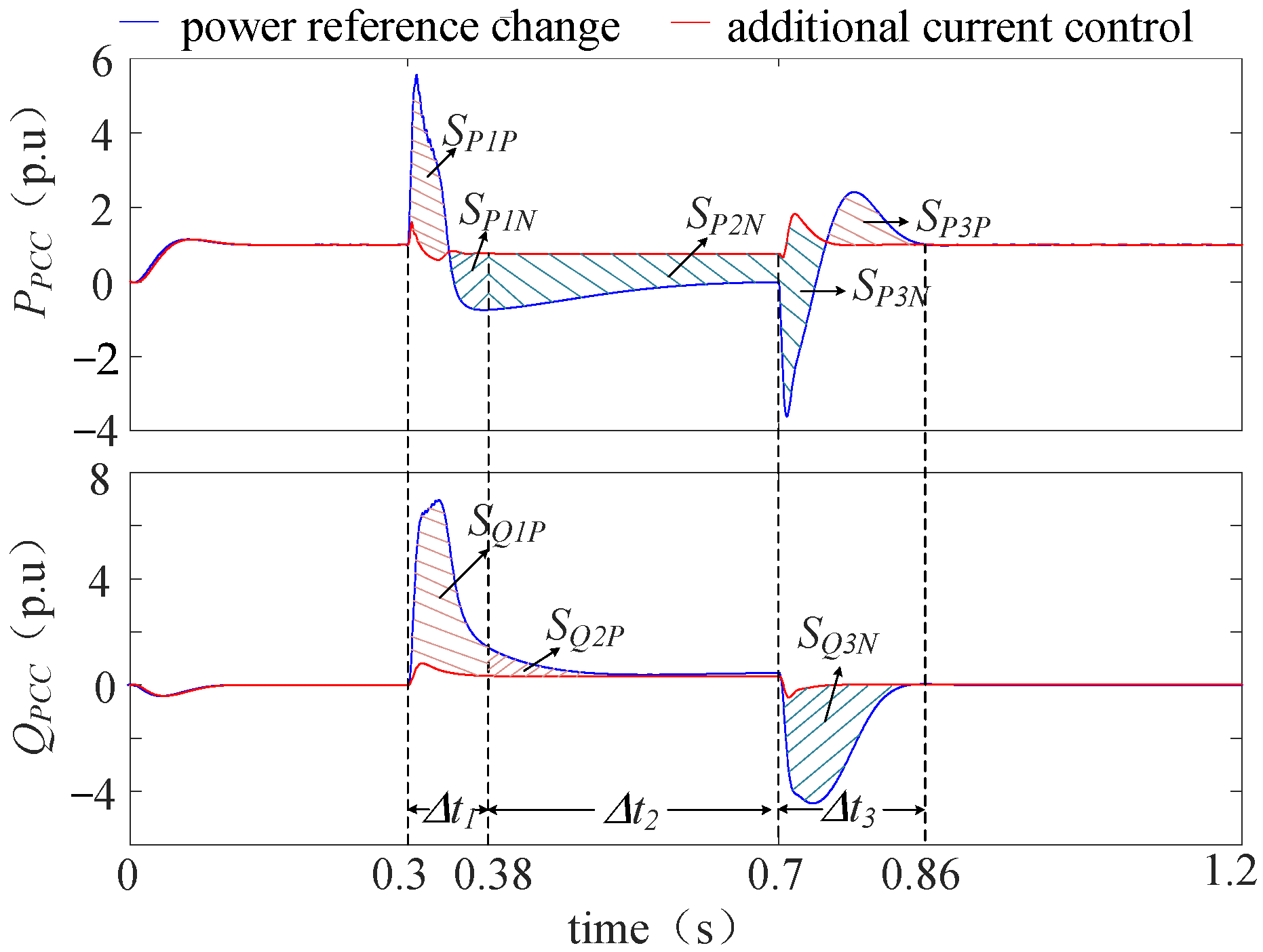
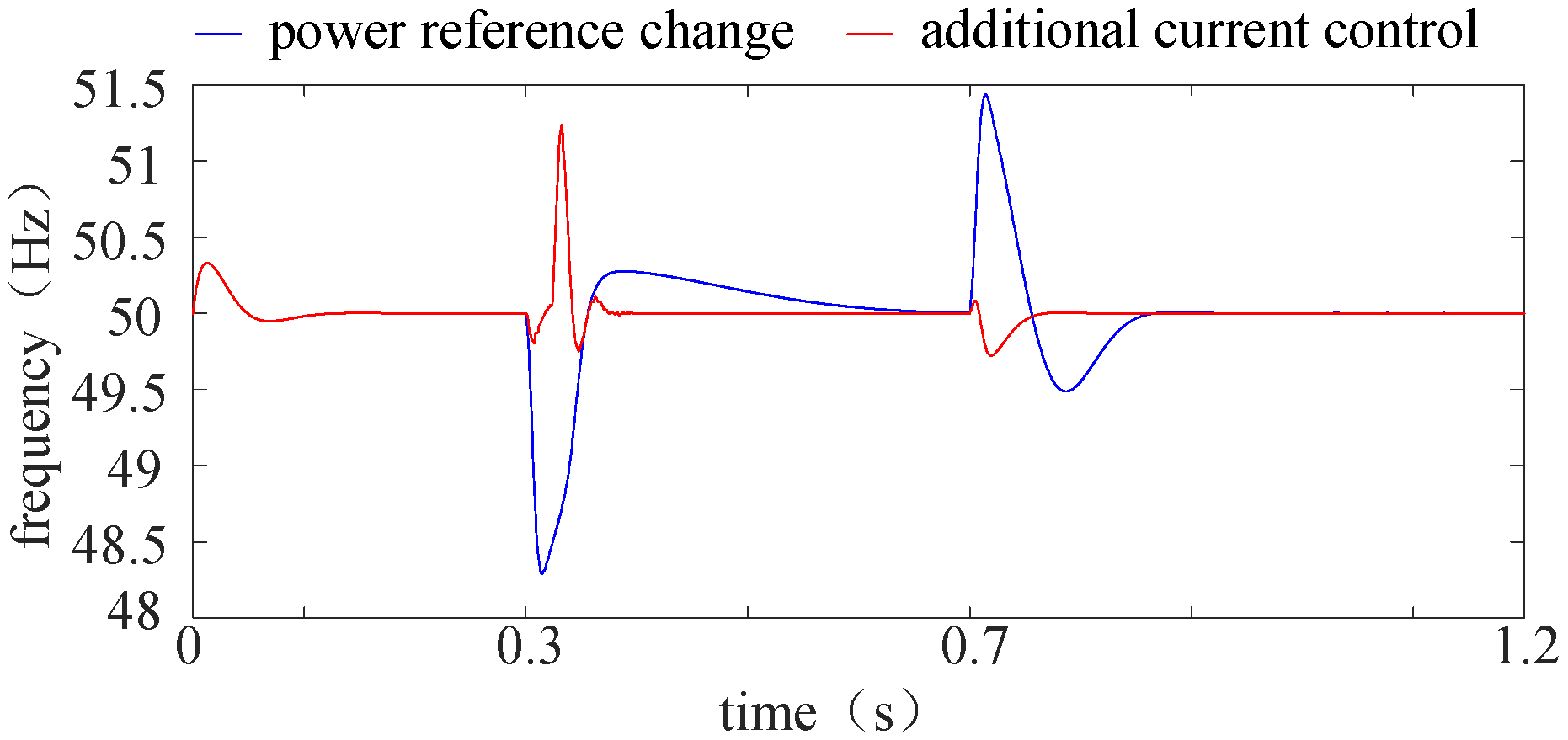
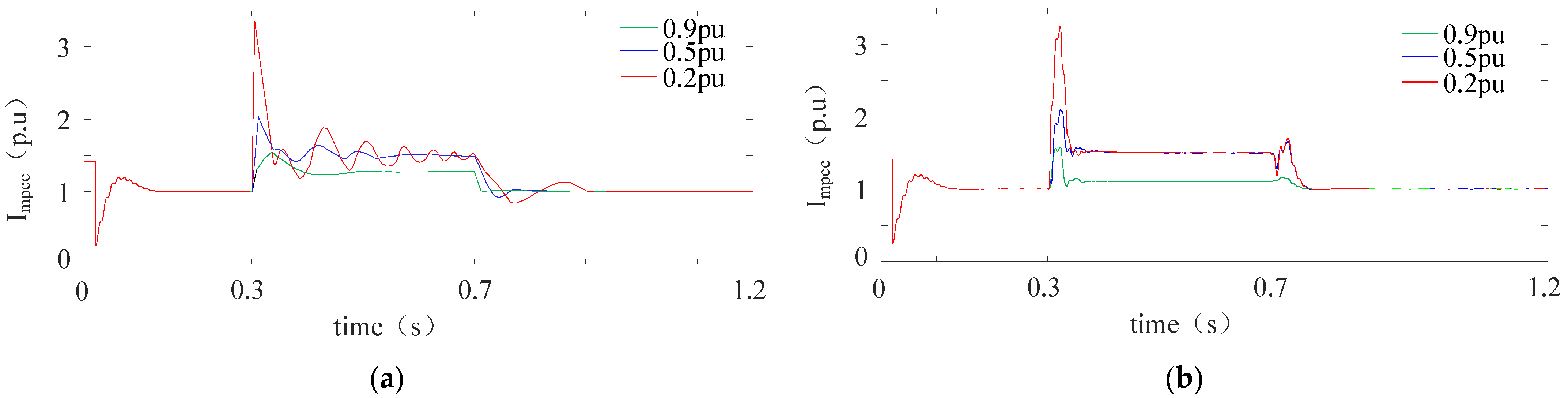
3.2. Comparative Analysis between Additional Current Control and Power Reference Changing

Depending on the degree of voltage dip detected, the rated capacity of the converter is changed as [16],

$$S_{new}=u_{pccpu}{S}_n$$

(15)

The reactive and active power reference are calculated based on the new converter rated capacity and voltage dip and can be expressed as,

$$Q_{refpu}^{\prime }=\left\{\begin{array}{l}1-u_{pccpu},\left(u_{pccpu}>0.9\right)\\ 2S_{new}\left(1-u_{pccpu}\right),\left(0.5\le u_{pccpu}\le 0.9\right)\\ S_{new},\left(u_{pccpu}<0.5\right)\end{array}\right.$$

(16)

$$P_{refpu}^{\prime }=\sqrt{S_{new}^2-Q_{refpu}^{\prime }{}^2}$$

(17)

Taking a grid voltage drop of 0.5 pu as an example, the reactive power reference can be calculated by Equation (16) as 0.5 pu, and the active reference is 0. Figure 7, Figure 8 and Figure 9 illustrate the changes of electric quantities during the fault.

Figure 7 shows that during Δt₁ (0.08 s), the PCC voltage amplitude of power reference changing is greater than the proposed additional current control, corresponding to Figure 8, the higher PCC voltage amplitude needs more energy (S_P1P + S_Q1P − S_P1N) supplied by converters. However, the active and reactive power output of the converter during this period of increasing PCC voltage amplitude is much greater than the rated capacity, which may cause equipment damage. During the Δt₂ (0.32 s), the PCC voltage amplitude under the additional current control is higher because of the larger active output and can provide more energy (S_P2N − S_Q2P). When t = 0.7 s, the fault recovers, but the voltage recovery process of power reference changing is slow because of the big difference between the normal and fault operation state, resulting in power feedback. Furthermore, the trend of the power output curve in Figure 8 shows that the additional current control (red line) can provide stable power output for the system within 0.1 s after the fault due to its good dynamic response.

Figure 9 shows that the frequency deviation is smaller and more stable because the additional current control is faster and closer to the actual value during the fault period.

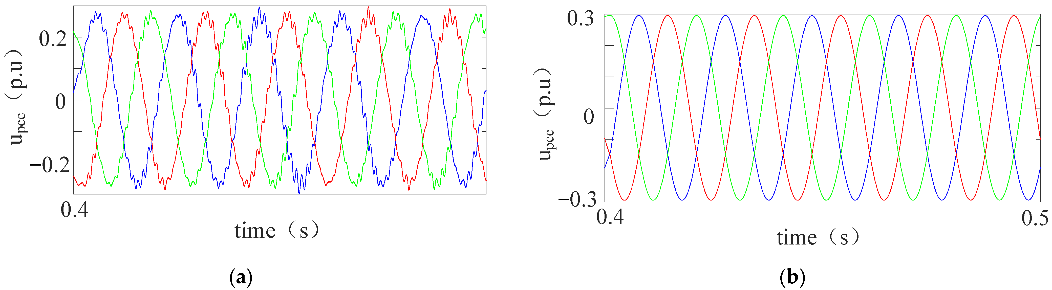
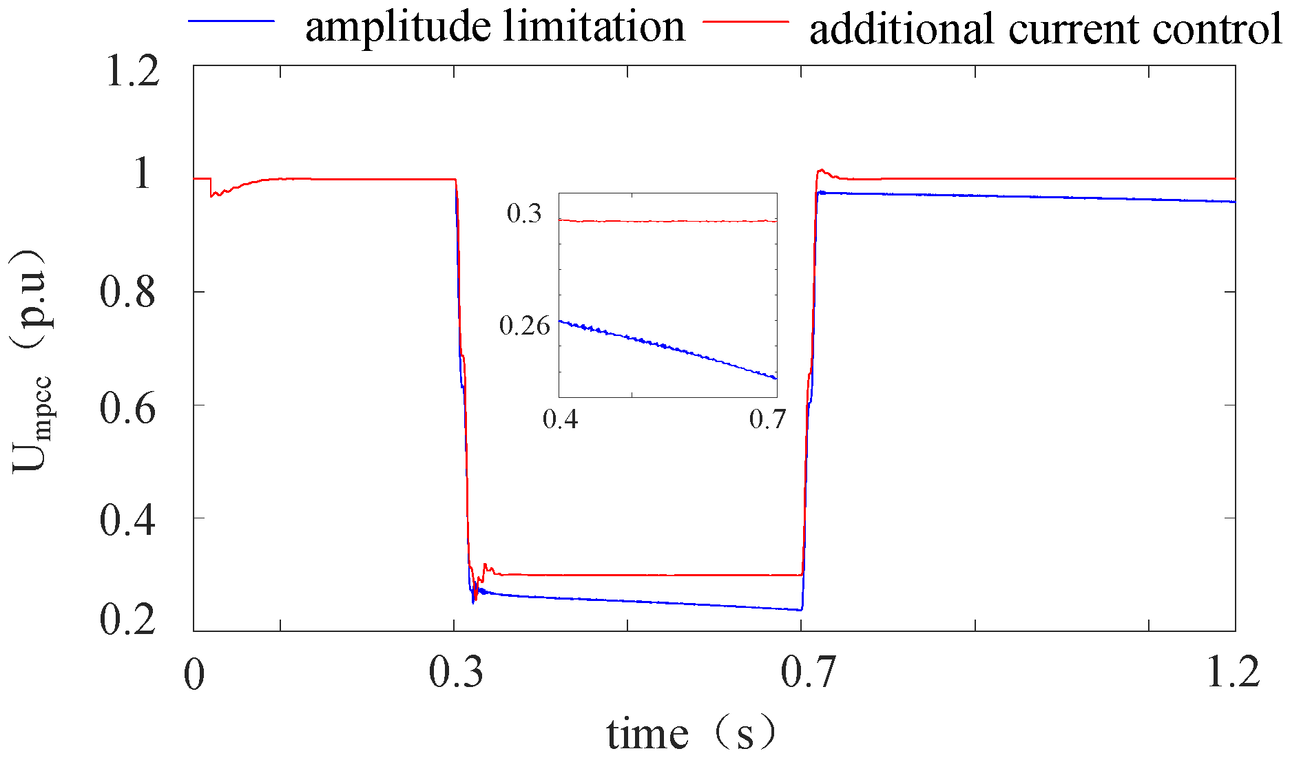
3.3. Comparative Analysis between Additional Current Control and Amplitude Limitation

Setting the current limiter directly after the voltage outer loop may cause system instability, thus the current reference used in current amplitude limitation is set by Equations (11) and (12). Thus, the converter is operated as a current source when the output current exceeds the limit. Taking a grid voltage drop of 0.2 pu as an example, the variation of each electrical quantity during the fault is found and is shown in the figure below.

Current amplitude limitation cannot control voltage effectively for its current source characteristic during faults. As seen in Figure 10, the voltage distortion under current amplitude limitation is serious, will increase the power loss and affect its fault ride-through capabilities, corresponding to Figure 11 (blue line), it can be seen that the converter export voltage during the fault can not be effectively controlled and be in a decreasing trend.According to the simulation of the proposed control strategy, the voltage waveform under fault is relatively stable, which can provide higher and more stable voltage support for PCC.

Another problem of the current amplitude limitation is the integral accumulation of outer voltage loop during fault. The system will become unstable if the current limiting is directly switched to the previous control mode. As illustrated in Figure 11, the voltage cannot recover to the set value.

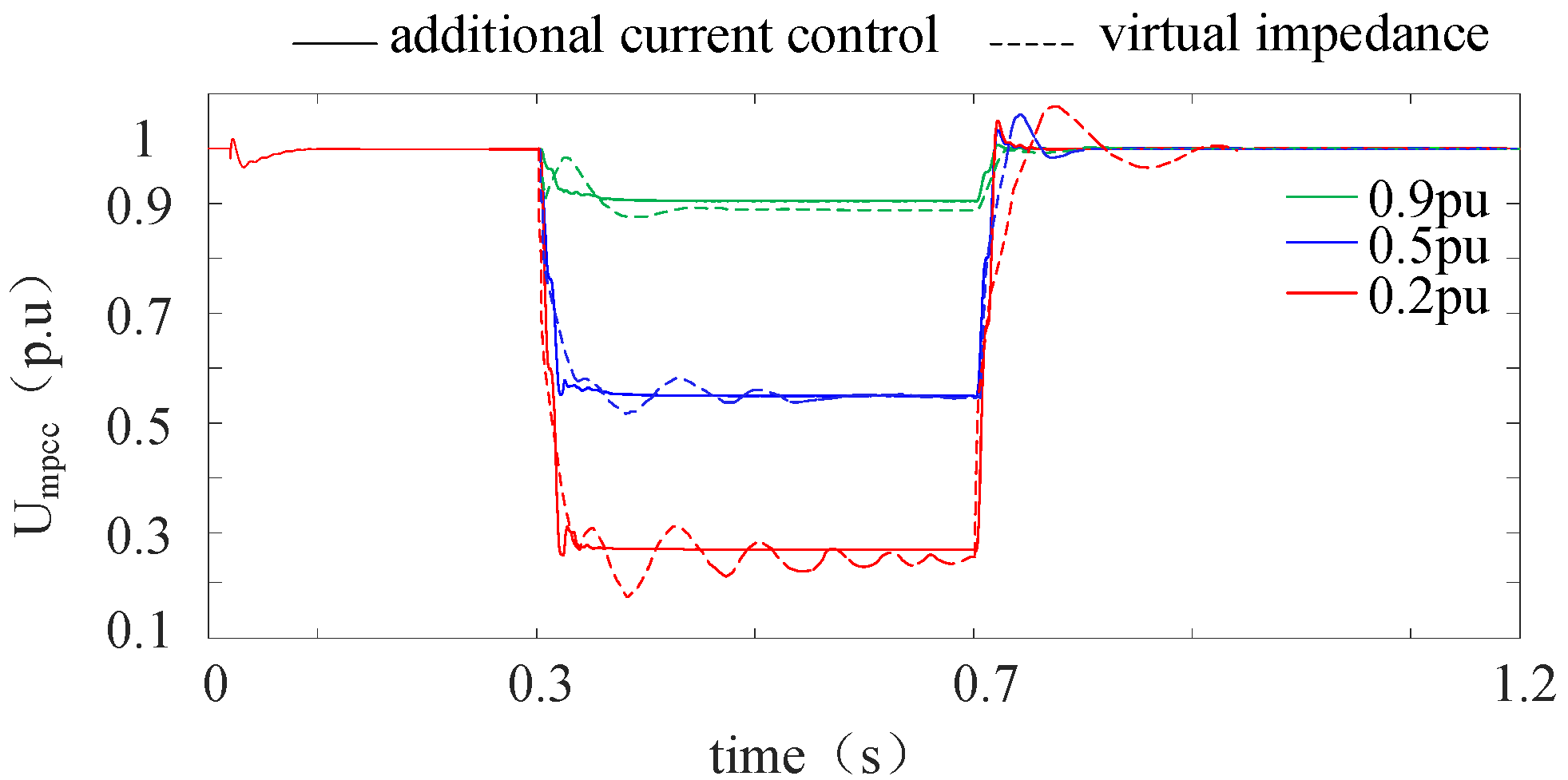
3.4. Comparative Analysis between Additional Current Control and Virtual Impedance

Taking the virtual impedance design method in [21] as the reference, the output current and voltage results under the two control methods are found and are shown in Figure 12 and Figure 13.

In Figure 12a, the amplitude of output current under virtual impedance control fluctuates seriously with the increase of voltage sag, reducing the current response speed. When the grid voltage drops to 0.2 pu, the virtual impedance control stabilizes the current around the set value in 0.4 s after the fault. In addition, the output current of the converter fluctuates, resulting in an unstable voltage at the PCC (dotted line in Figure 13). Compared with the virtual impedance, the proposed additional current control can realize the rapid control of the current under different voltage sags, stabilize the current at the set value within 0.1 s, and provide stable voltage support for the grid.

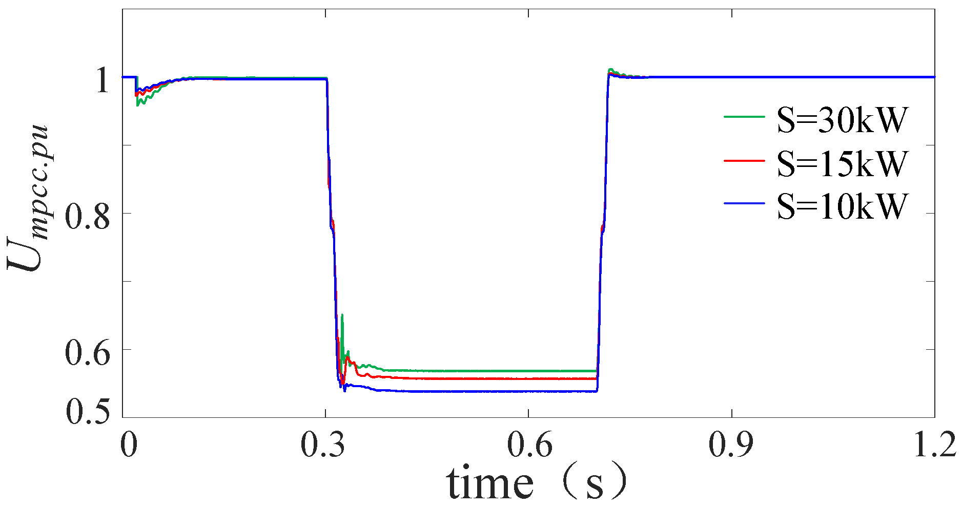
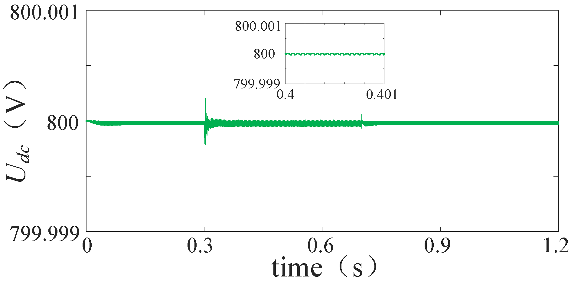
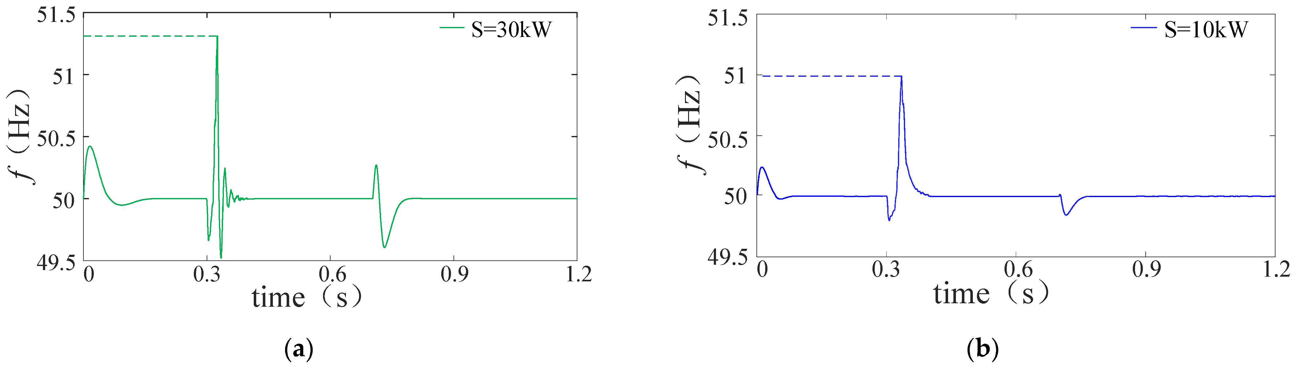
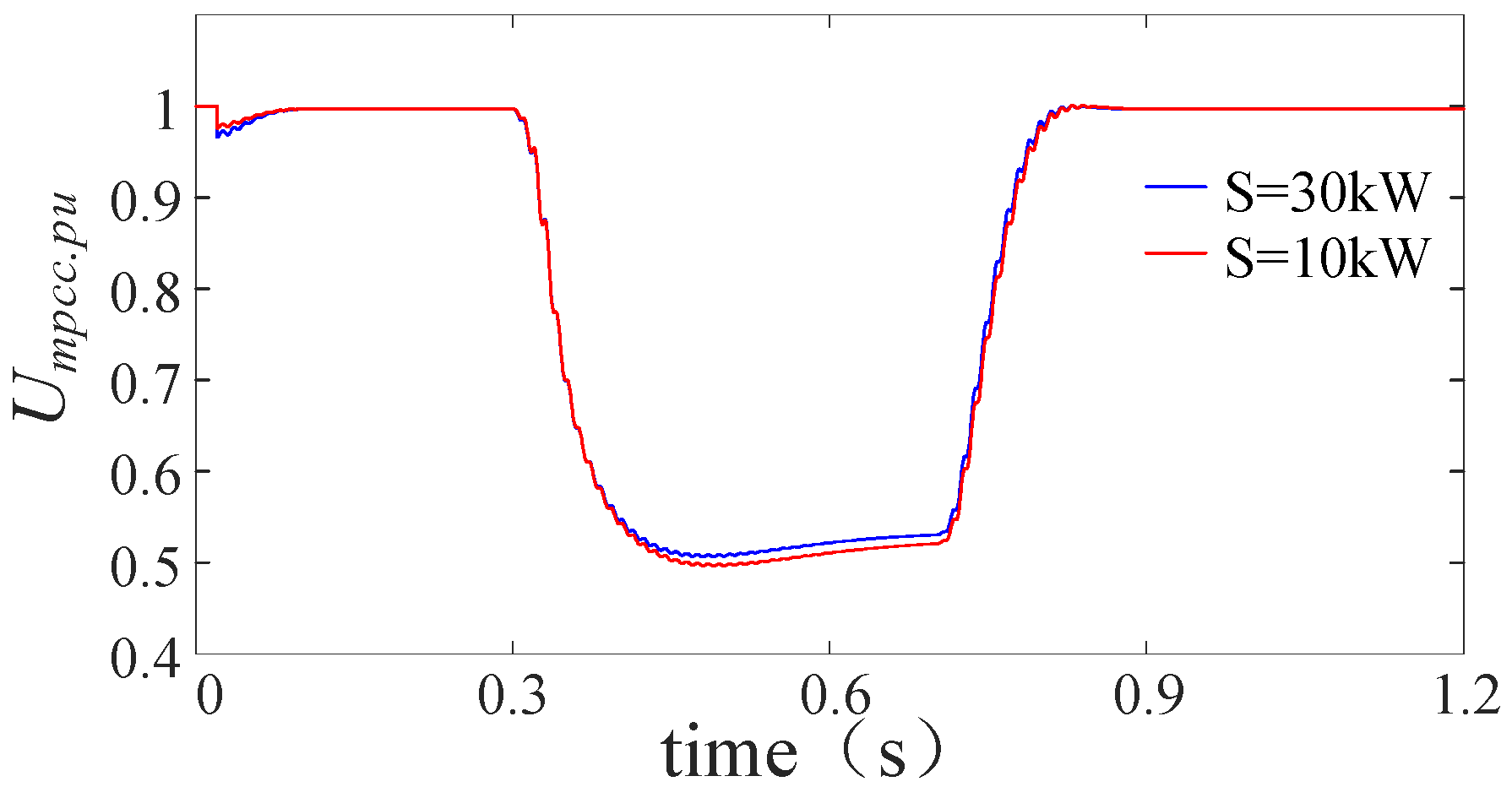
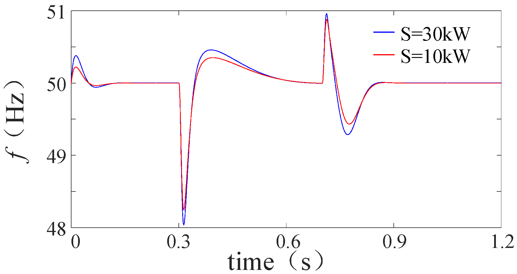
3.5. Current Limitation Effect under Different Capacities

To further verify the effectiveness of the proposed strategy, the strategy is applied to different converter capacities to observe its control performance and the performance is shown in Figure 14, Figure 15 and Figure 16. For comparison, the conventional control effect without current limiting strategy is shown in Figure 17 and Figure 18.

The voltage and frequency response curves in Figure 17 and Figure 18 show that the conventional control is unable to change quickly and meet the output requirements of the converters during the fault scenarios. This inability is because the original control target remains unchanged. Thus, there will be a large frequency and voltage dip, thus the control cannot provide a smooth voltage support for the system.

From Figure 14, Figure 15 and Figure 16, it can be shown that different capacity converters can be stabilized within 0.1 s under fault scenarios using the control method proposed in this paper. The proposed method has the following three main advantages compared with conventional control.

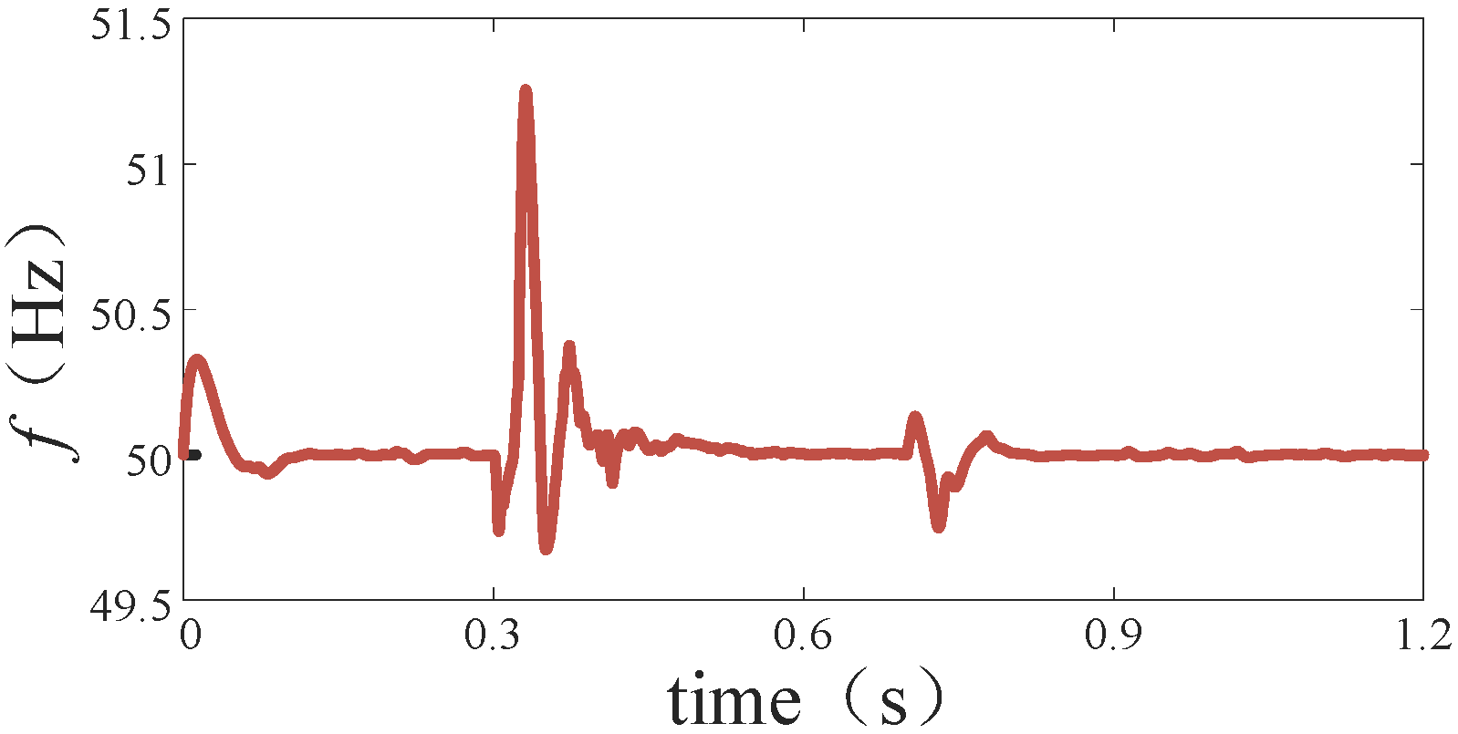
• Fast response speed: the proposed control can achieve stability within 0.1 s after a fault.
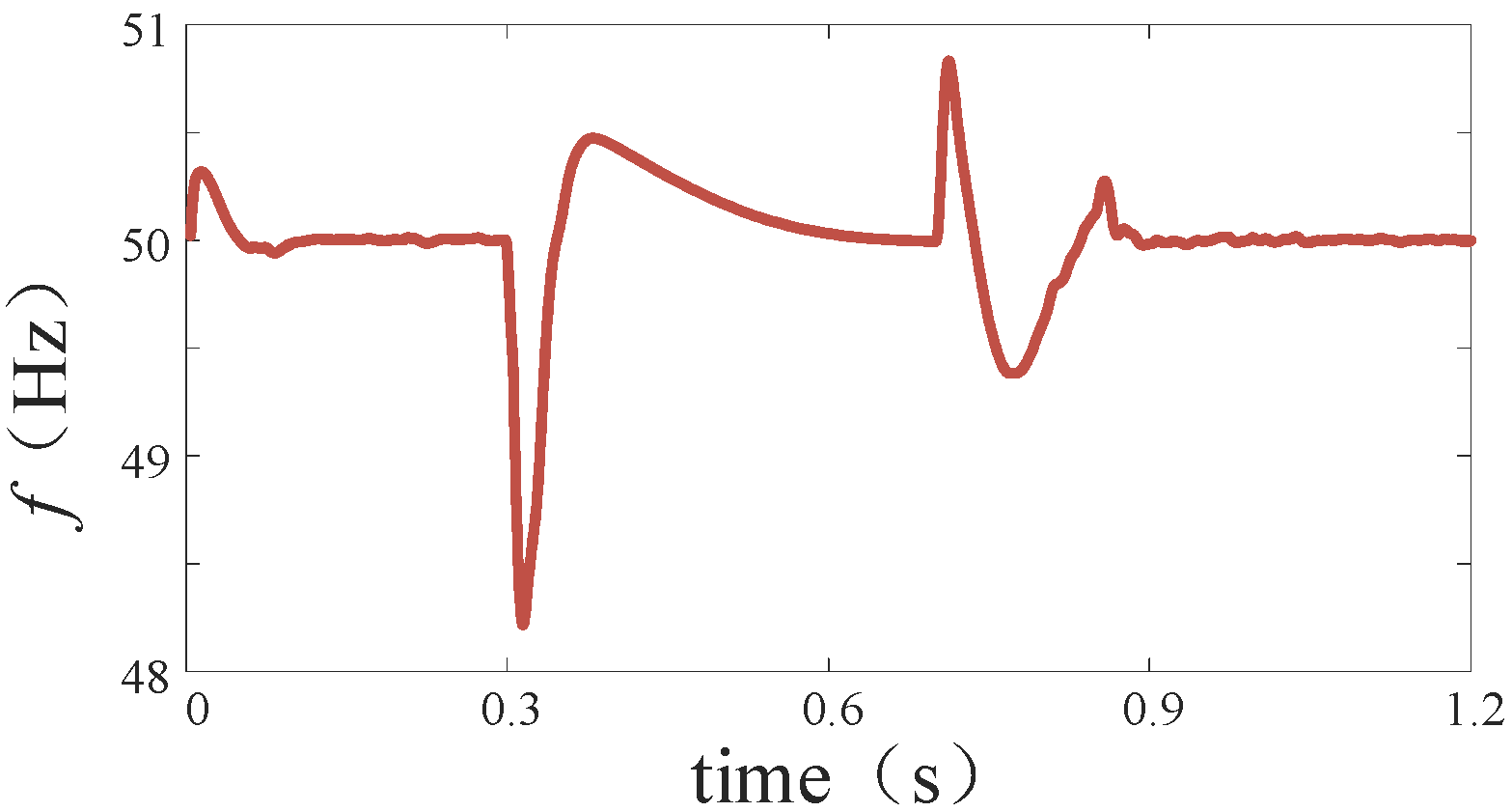
• The control method proposed in this paper can maintain the frequency deviation within 1.5 Hz compared to a frequency change of 2 Hz under a conventional controller.
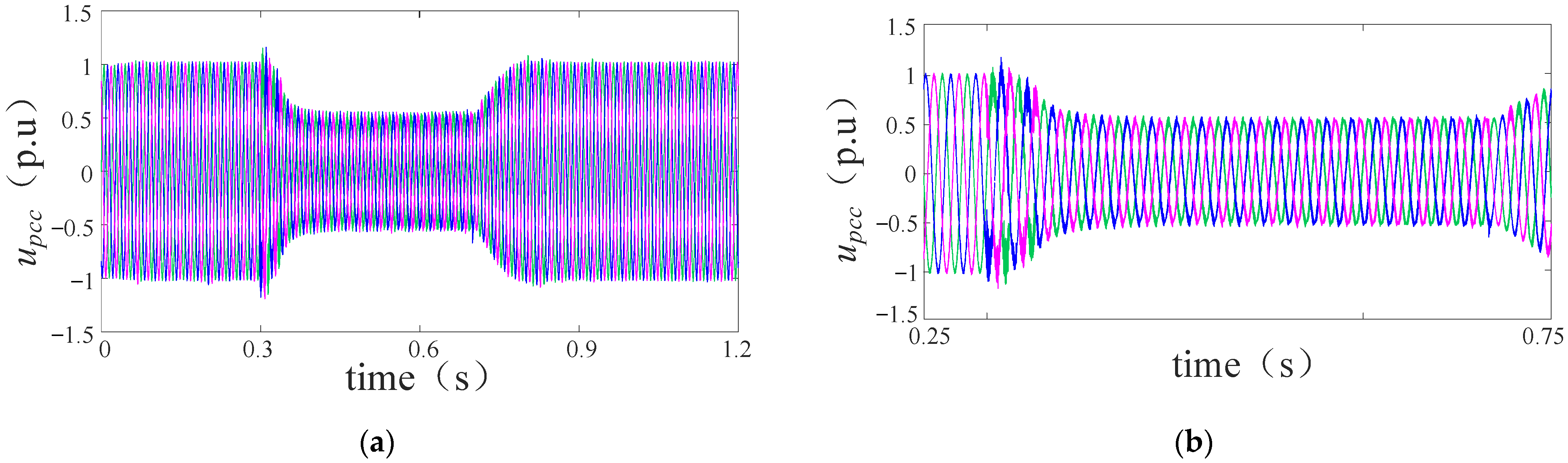
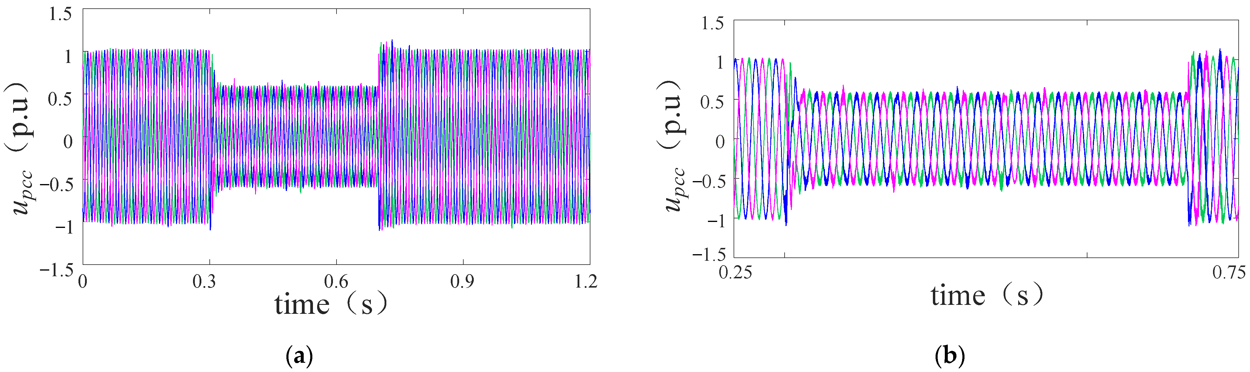
• The proposed control can promote voltage stabilization faster than a conventional controller and keep the voltage at a higher level. Hence, the proposed control can provide uninterrupted voltage support for the grid and facilitate fault recovery.

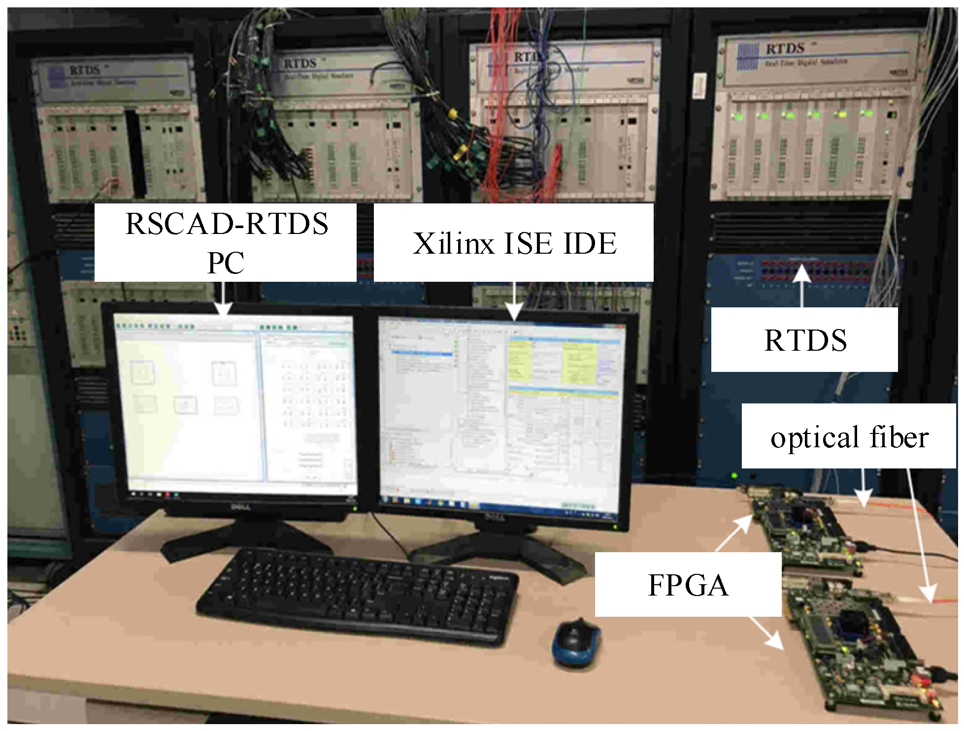
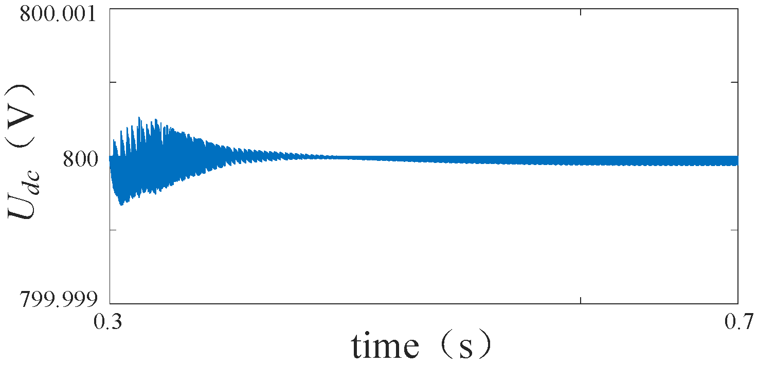
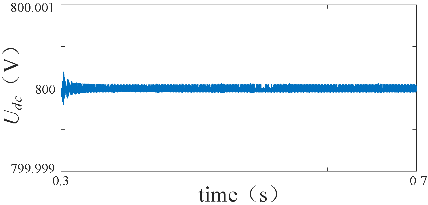
4. HIL Validation

To further verify the effectiveness of the proposed current limiting strategy, the strategy has been validated through hardware-in-the-loop experiments using an RTDS platform. The hardware set-up is shown in Figure 19. This research selected the Xilinx Virtex-6 series ML605 integrated development board. The research also used the Verilog HDL hardware description language to develop and implement the control strategy proposed in this paper under Xilinx ISE 14.7 integrated development environment. Finally, the modulation wave was generated by an FPGA board. The communication connection between the FPGA board and RTDS was established through an optical fiber.

The control effect after the application of the proposed strategy and under the conventional control are shown in Figure 20, Figure 21, Figure 22, Figure 23, Figure 24 and Figure 25. The experimental results are in good agreement with the simulation that the proposed control has better stability during the fault and enables fault recovery.

5. Conclusions

Aiming to solve the overcurrent caused by three-phase symmetrical faults, this paper proposed a current limiting method for GFM converter with low-pass filtering and additional current loop.

By adopting the proposed method, the decay rate of current is accelerated to reach the set value quickly. At the same time, this method ensures the voltage source characteristics of GFM and provides continuous and stable voltage support for the grid. The addition of low-pass filtering solves the problem of frequencies beyond the limit caused by the instantaneous input of the active additional current loop and smooths the frequency fluctuations. Furthermore, the proposed strategy makes full use of the capacity margin of the converter and provides voltage support during the fault period while ensuring the active transmission capacity to the greatest extent.

References

1. Huang, L.B.; Xin, H.H.; Ju, P.; Hu, J.B. Synchronization Stability Analysis and Unified Synchronization Control Structure of Grid-connected Power Electronic Devices. Electr. Power Autom. Equip. 2020, 40, 10–25. [Google Scholar]
2. Cen, Y.; Huang, M.; Zha, X.M. The Transient Response Analysis of SRF-PLL under the Unbalance Grid Voltage Sag. Trans. China Electrotech. Soc. 2016, 31, 28–38. [Google Scholar]
3. Pattabiraman, D.; Lasseter, R.H.; Jahns, T.M. Comparison of Grid Following and Grid Forming Control for a High Inverter Penetration Power System. In Proceedings of the 2018 IEEE Power & Energy Society General Meeting (PESGM), Portland, OR, USA, 5–10 August 2018; pp. 1–5. [Google Scholar]
4. Rosso, R.; Wang, X.; Liserre, M.; Lu, X.; Engelken, S. Grid-Forming Converters: Control Approaches, Grid-Synchronization, and Future Trends—A Review. IEEE Open J. Ind. Appl. 2021, 2, 93–109. [Google Scholar] [CrossRef]
5. Ackermann, T.; Prevost, T.; Vittal, V.; Roscoe, A.J.; Matevosyan, J.; Miller, N. Paving the Way: A Future Without Inertia Is Closer Than You Think. IEEE Power Energy Mag. 2017, 15, 61–69. [Google Scholar] [CrossRef] [Green Version]
6. Erickson, M.J. Improved Power Control of Inverter Sources in Mixed-Source Micro-Grids; The University of Wisconsin-Madison: Madison, WI, USA, 2012. [Google Scholar]
7. Shuai, Z.; Huang, W.; Shen, C.; Ge, J.; Shen, Z.J. Characteristics and Restraining Method of Fast Transient Inrush Fault Currents in Synchronverters. IEEE Trans. Ind. Electron. 2017, 64, 7487–7497. [Google Scholar] [CrossRef]
8. Taoufik, Q.; François, G.; Fréderic, C.; Guillaume, D.; Thibault, P.; Xavier, G. Critical Clearing Time Determination and Enhancement of Grid-Forming Converters Embedding Virtual Impedance as Current Limitation Algorithm. IEEE J. Emerg. Sel. Top. Power Electron. 2020, 8, 1050–1061. [Google Scholar]
9. Qoria, T.; Gruson, F.; Colas, F.; Denis, G.; Prevost, T.; Guillaud, X.A. Current Limiting Strategy to Improve Fault Ride-Through of Inverter Interfaced Autonomous Micro-grids. IEEE Trans. Smart Grid 2017, 8, 2138–2148. [Google Scholar]
10. Yu, M.; Huang, W.; Tai, N.; Zheng, X.; Wu, P.; Chen, W. Transient Stability Mechanism of Grid-connected Inverter-interfaced Distributed Generators Using Droop Control Strategy. Appl. Energy 2018, 210, 737–747. [Google Scholar] [CrossRef]
11. Zhong, Q.C.; Konstantopoulos, G.C. Current-Limiting Droop Control of Grid-Connected Converters. IEEE Trans. Ind. Electron. 2017, 64, 5963–5973. [Google Scholar] [CrossRef] [Green Version]
12. Paquette, A.D.; Divan, D.M. Virtual Impedance Current Limiting for Converters in Micro-grids with Synchronous Generators. IEEE Trans. Ind. Appl. 2015, 51, 1630–1638. [Google Scholar] [CrossRef]
13. He, J.; Li, Y.W. Analysis, Design and Implementation of Virtual Impedance for Power Electronics Interfaced Distributed Generation. IEEE Trans. Ind. Appl. 2011, 47, 2525–2538. [Google Scholar] [CrossRef]
14. Wang, X.M.; Wang, Y.B.; Liu, Y.T.; Liu, C.; Wang, S.J.; Hu, B. Low Voltage Ride Through Control Method of Actively Supported New Energy Unit Based on Virtual Reactance. Power Syst. Technol. 2022, 46, 4435–4444. [Google Scholar]
15. Li, Y.W.; Vilathgamuwa, D.M.; Loh, P.C.; Blaabjerg, F. A Dual-Functional Medium Voltage Level DVR to Limit Downstream Fault Currents. IEEE Trans. Power Electron. 2007, 22, 1330–1340. [Google Scholar] [CrossRef]
16. Afshari, E.; Moradi, G.R.; Rahimi, R.; Farhangi, B.; Yang, Y.; Blaabjerg, F.; Farhangi, S. Control Strategy for Three-Phase Grid-Connected PV Converters Enabling Current Limitation Under Unbalanced Faults. IEEE Trans. Ind. Electron. 2017, 64, 8908–8918. [Google Scholar] [CrossRef] [Green Version]
17. Taul, M.G.; Wang, X.; Davari, P.; Blaabjerg, F. Current Limiting Control with Enhanced Dynamics of Grid-Forming Converters During Fault Conditions. IEEE J. Emerg. Sel. Top. Power Electron. 2020, 8, 1062–1073. [Google Scholar] [CrossRef] [Green Version]
18. Wu, H.; Wang, X. Transient Stability Analysis of Grid-connected Converter System Considering Frequency Disturbance of Power Grid. Autom. Electr. Power Syst. 2021, 45, 78–84. [Google Scholar]
19. Xi, L.Y.; Wang, J.F.; Hou, C.C.; Qiu, Z.L. Design of phase locked loop based on third-order general-integrator. Power Syst. Prot. Control 2016, 44, 184–189. [Google Scholar]
20. Glöckler, C.; Duckwitz, D.; Welck, F. Virtual Synchronous Machine Control with Virtual Resistor for Enhanced Short Circuit Capability. In Proceedings of the 2017 IEEE PES Innovative Smart Grid Technologies Conference Europe (ISGT-Europe), Turin, Italy, 26–29 September 2017; pp. 1–6. [Google Scholar]
21. Welck, F.; Duckwitz, D.; Gloeckler, C. Influence of Virtual Impedance on Short Circuit Performance of Virtual Synchronous Machines in the 9-Bus System. In Proceedings of the NEIS 2017, Conference on Sustainable Energy Supply and Energy Storage Systems, Hamburg, Germany, 21–22 September 2017; pp. 1–7. [Google Scholar]
22. Gkountaras, A.; Dieckerhoff, S.; Sezi, T. Evaluation of Current Limiting Methods for Grid Forming Converters in Medium Voltage Micro-grids. In Proceedings of the 2015 IEEE Energy Conversion Congress and Exposition (ECCE), Montreal, QC, Canada, 20–24 September 2015; pp. 1223–1230. [Google Scholar]
23. Zhong, Q.C. Virtual Synchronous Machines and Autonomous Power Systems. Proc. CSEE 2017, 37, 336–348. [Google Scholar]
24. Lan, Z.; Long, Y.; Zeng, J.H.; Tu, C.M.; Xiao, F.; Guo, Q. Transient Power Oscillation Suppression Strategy of Virtual Synchronous Generator Considering Overshoot. Autom. Electr. Power Syst. 2022, 46, 131–141. [Google Scholar]
25. Remon, D.; Cantarellas, A.M.; Rakhshani, E.; Candela, I.; Rodriguez, P. An Active Power Synchronization Control Loop for Grid-connected Converters. In Proceedings of the 2014 IEEE PES General Meeting|Conference & Exposition, National Harbor, MD, USA, 27–31 July 2014; pp. 1–5. [Google Scholar]
26. Rodríguez, P.; Citro, C.; Candela, J.I.; Rocabert, J.; Luna, A. Flexible Grid Connection and Islanding of SPC-based PV Power Converters. IEEE Trans. Ind. Appl. 2018, 54, 2690–2702. [Google Scholar] [CrossRef]
27. Zhang, Z.K.; Huang, Z.; Chi, Y.N.; Wang, J.; Li, Y. Explanation of Technical Rule for Connecting Offshore Wind Farm into Power Grid. Smart Grid. 2016, 4, 345–350. [Google Scholar]
Figure 1. The main topology and control blocks of the GFM converter.
Electronics 12 01112 g001
Figure 2. The improved control loop of GFM.
Electronics 12 01112 g002
Figure 3. The structure of low-pass filter.
Electronics 12 01112 g003
Figure 4. Amplitude and phase frequency characteristic curves of low-pass filter.
Electronics 12 01112 g004
Figure 5. The improved control loop of reactive power.
Electronics 12 01112 g005
Figure 6. The improved topology and control blocks of the GFM converter.
Electronics 12 01112 g006
Figure 7. Comparison chart of PCC voltage amplitude.
Electronics 12 01112 g007
Figure 8. Comparison chart of output power.
Electronics 12 01112 g008
Figure 9. Comparison chart of frequency.
Electronics 12 01112 g009
Figure 10. Comparison of PCC voltage: (a) PCC voltage under current amplitude limitation and (b) PCC voltage under additional current control.
Electronics 12 01112 g010
Figure 11. Comparison of PCC voltage amplitude under amplitude limitation and additional current control.
Electronics 12 01112 g011
Figure 12. Comparison of output current amplitude: (a) output current amplitude under virtual impedance control and (b) output current amplitude under additional current control.
Electronics 12 01112 g012
Figure 13. Comparison of PCC voltage amplitude under virtual impedance and additional current control.
Electronics 12 01112 g013
Figure 14. Voltage magnitude curve under additional current control at different capacities.
Electronics 12 01112 g014
Figure 15. DC capacitor terminal voltage.
Electronics 12 01112 g015
Figure 16. Frequency curve under additional current control: (a) converter capacity, SN = 30 kW and (b) converter capacity, SN = 10 kW.
Electronics 12 01112 g016
Figure 17. Voltage magnitude curve under conventional control at different capacities.
Electronics 12 01112 g017
Figure 18. Frequency curve under conventional control at different capacities.
Electronics 12 01112 g018
Figure 19. Configuration of the experimental platform.
Electronics 12 01112 g019
Figure 20. DC capacitor terminal voltage under conventional control.
Electronics 12 01112 g020
Figure 21. DC capacitor terminal voltage under additional current control.
Electronics 12 01112 g021
Figure 22. Frequency under conventional control.
Electronics 12 01112 g022
Figure 23. Frequency under additional current control.
Electronics 12 01112 g023
Figure 24. Voltage curve under conventional control: (a) voltage of the whole experiment and (b) voltage between t = 0.25–0.75 s after magnification.
Electronics 12 01112 g024
Figure 25. Voltage curve under additional current control: (a) voltage of the whole experiment and (b) voltage between t = 0.25–0.75 s after magnification.
Electronics 12 01112 g025