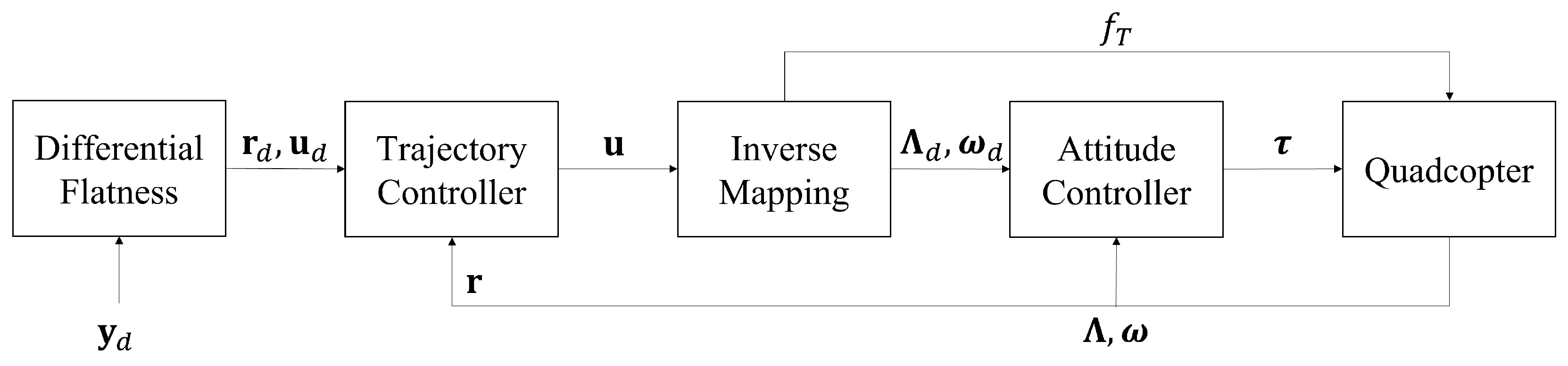
Article

EKF-SLAM for Quadcopter Using Differential Flatness-Based LQR Control

1
Department of Aerospace Engineering & Engineering Mechanics, University of Cincinnati, Cincinnati, OH 45221, USA
2
Department of Mechanical & Materials Engineering, University of Cincinnati, Cincinnati, OH 45221, USA
*
Author to whom correspondence should be addressed.
Electronics 2023, 12(5), 1113; https://doi.org/10.3390/electronics12051113
Submission received: 21 January 2023 / Revised: 9 February 2023 / Accepted: 17 February 2023 / Published: 24 February 2023

Abstract

:
SLAM (Simultaneous Localization And Mapping) in unmanned aerial vehicles can be an advantageous proposition during dangerous missions where aggressive maneuvers are paramount. This paper proposes to achieve it for a quadcopter using a differential flatness-based linear quadratic regulator while utilizing sensor measurements of an inertial measurement unit and light detection and ranging considering sensors’ constraints, such as a limited sensing range and field of view. Additionally, a strategy to reduce the computational effort of Extended Kalman Filter-based SLAM (EKF-SLAM) is proposed. To validate the performance of the proposed approach, this work considers a quadcopter traversing an 8-shape trajectory for two scenarios of known and unknown landmarks. The estimation errors for the quadcopter states are comparable for both cases. The accuracy of the proposed method is evident from the Root-Mean-Square Errors (RMSE) of 0.04 m, 0.04 m/s, and 0.34 deg for the position, velocity, and attitude estimation of the quadcopter, respectively, including the RMSE of 0.03 m for the landmark position estimation. Lastly, the averaged computational time for each step of EKF-SLAM with respect to the number of landmarks can help to strategically choose the respective number of landmarks for each step to maximize the use of sensor data and improve performance.

1. Introduction

SLAM (Simultaneous Localization And Mapping) aims to solve the problem of localization of an autonomous robot in an unknown environment by simultaneously mapping the surroundings. The emergence of indoor applications of mobile robotics has made SLAM an attractive alternative to user-built maps [1]. Moreover, SLAM is gradually finding applications outdoors, underwater, and in space devoid of a Global Positioning System (GPS) [2]. Essentially, SLAM can be divided into a process of front-end and back-end formulation, where the front-end comprises feature extraction, data association, and outlier rejection, whereas the back-end deals with the main estimation process of robot poses and landmark positions [1]. Based on factors, such as spatial representation, the structure and dynamics of the environment, and the employed sensors, a variety of approaches to SLAM can be used, which include but are not limited to GraphSLAM, FastSLAM, and VoSLAM [3].
Several developments have been made for mobile mapping systems using ground-based systems, but unmanned aerial vehicles (UAVs) could provide advantages at hazardous sites compared to other platforms and enable mapping at different resolutions with the ability to fly at different elevations and speeds [4]. For UAVs, the most popular method for SLAM implementation has been based on Extended Kalman Filter (EKF), that is EKF-SLAM, with a majority using Inertial Measurement Units (IMUs) as proprioceptive sensors and visual odometry-based sensors such as cameras as exteroceptive sensors [5]. The EKF-SLAM approach was first proposed by Smith et al. [6], where EKF is a Bayesian approach of estimation utilizing posterior probability distribution. EKF-SLAM faces key issues, especially in terms of computational effort as computation increases quadratically with the number of landmarks [7]. Still, EKF-SLAM is the most popular method with the ability to deal with non-linear systems, and plenty of available research and resources [8].
SLAM is basically solved specifically for vision-based slow robots in 2D indoor environments [1], but it is still an enigma for highly agile robots such as quadcopters, operating in indoor or outdoor environments. The SLAM algorithm has been studied for UAVs with 3D observations of LiDAR (Light Detection And Ranging) or comparable to LiDAR in a few research works [2,4,9,10,11,12]. Note that cameras are extremely sensitive to lighting conditions and have limitations in capturing the geometry of the observed scene and generating more accurate maps, thus a more effective sensor, LiDAR, is being considered more lately [4]. Cho and Hwang [9] conducted SLAM with just four landmarks using EKF-SLAM and observation in terms of range and attitude difference. In [10], 3D SLAM is performed for UAVs using a linear Kalman filter with the linearized model for the UAVs and range-bearing measurements. A data fusion algorithm was proposed for UAVs by the integration of LiDAR measurements with GPS to perform in GPS-degraded environments [11]. Kim et al. [12] discussed an application of LiDAR for the localization of speedy UAVs in a GPS-denied outdoor environment while conducting surface reconstruction and elevation registration. While all of the aforementioned studies have used EKF in some form, there are others. Sadeghzadeh-Nokhodberiz et al. [2] studied the application of 3D SLAM on UAVs using FastSLAM and LiDAR. Karam et al. [4] used LiDAR for validation of the performance of GraphSLAM using rangefinders on UAVs.
Most works discussed above are focused on localization and mapping and mostly have not discussed the control strategies used. Many of them used the most basic controller such as PID control with pre-defined control signals for following a set trajectory. In [13], SLAM was achieved using a sliding mode control for the non-linear system of a quadcopter, but still lacked the ability to closely follow a given trajectory over extended periods. Moreover, UAVs can have aggressive maneuvers where fast and reliable SLAM is required. Thus, this work proposes the use of a Differential Flatness-based Linear Quadratic Regulator (DF-LQR). It is known that LQR is an optimum control superior to other classical approaches including PID in terms of robustness, energy performance, computational efficiency, and tuning parameters [14]. However, LQR by itself can only be applied to linear or linearized systems. A DF-based approach, where the non-linear system of quadcopters can be formulated linearly for control using LQR, has been proposed to achieve aggressive maneuvers [15]. For UAVs operating in any dangerous conditions, aggressive maneuvers could be paramount and thus DF-based LQR control for quadcopters could be an ideal choice. In practice, control is achieved in SLAM based on control signals obtained using estimated states rather than true-value states, but many researchers have been conducting studies assuming true-value states [2,9,10]. DF-based LQR control has not been studied in conjunction with 3D SLAM, and thus this work proposes to do so while also calculating control signals from estimated states. The effectiveness of this control strategy is validated by comparing the results of estimated quadcopter states when landmarks are unknown and are also being estimated to a case when landmarks are known.
As mentioned previously, EKF-SLAM is computationally intensive with the increasing number of landmarks, but it is still a method of choice for several researchers, as is evident from several kinds of research over the years using EKF [8]. While there has been research on reducing the computational complexity of EKF-SLAM with the use of local maps for 2D motion [16], it would be beneficial if there are metrics that can provide inference on computation time for different steps of SLAM, such as prediction, update, and registration such that decisions can be made on the size of map space for predictions, the number of landmarks for update, or registration, or even the time step for SLAM. This work proposes a strategy to reduce the computational effort of EKF-SLAM, which is tightly combined with the UAV control discussed above. It conducts multiple simulations over different numbers of landmarks to study the relationship between these time parameters with the landmarks in consideration. Although these metrics were derived for the specific computing resources available in this study, comparable metrics can be derived for other computing resources in use. Therefore, it is thought that it can provide direction to researchers who want to use or improve EKF-SLAM in the future.
In summary, the contributions of this paper are summarized below:
  • Study of DF-based LQR control in 3D EKF-SLAM to achieve a better and more realistic trajectory control using estimated states.
  • A pragmatic way of using LiDAR measurements as they become available based on UAV position and LiDAR’s Field Of View (FOV).
  • Inducing decision-making to improve the computational efficiency of the appropriate number of landmarks or EKF-SLAM through the development of a metric of the relationship between the number of landmarks and the time step.

2. Methodologies

2.1. Dynamic and Kinematic Model of Quadcopters

The inertial and body frames and the state variables to describe the motion of the quadcopter are depicted in Figure 1. The inertial frame N, which is fixed to the surface of the Earth at mean sea level, is defined as n ^ i for i = 1, 2, and 3, where n ^ 1 is directed towards North, n ^ 2 is directed towards East, and n ^ 3 points to the center of the Earth. Note that one assumes a flat, non-rotating Earth with a uniform gravitational field. The body frame B, whose origin is fixed to the center of gravity of the quadcopter, is defined as b ^ i for i = 1, 2, and 3, where b ^ 1 is directed normal to the field of view of the LiDAR on the quadcopter, b ^ 2 points to the direction of the right arm of the quadcopter, and b ^ 3 is directed downwards, which is perpendicular to the quadcopter plane.
The quadcopter is assumed to be an exactly symmetrical rigid body, which implies that the inertia matrix is diagonal, with 3 Degrees-Of-Freedom (DOF) translation motion and 3 DOF rotational motion. The quadcopter’s attitude with respect to the inertial frame is expressed using the 3-2-1 set of the Euler angles as ϕ , θ , and ψ that represent the roll, pitch, and yaw angles, respectively. Note that the direction cosine matrix that maps from the body frame to the inertial frame is described as [17]:
C N B   =   C 3 ( ψ ) C 2 ( θ ) C 1 ( ϕ ) .
Note that each direction cosine matrix is defined as
C 3 ( ψ )   =   c ψ s ψ 0 s ψ c ψ 0 0 0 1 , C 2 ( θ )   =   c θ 0 s θ 0 1 0 s θ 0 c θ , C 1 ( ϕ )   =   1 0 0 0 c ϕ s ϕ 0 s ϕ c ϕ .
where, for instance, c ψ and s ψ are cos ψ and sin ψ , respectively.
To describe the motion of the quadcopter, this work defines a state model as [18]:
N ρ ˙ B ν ˙ B Λ ˙ B ω ˙   =   C N B B ν B ω   ×   B ν   +   C N B T N f g   +   B f T / m D B ω J 1 B ω   ×   J B ω   +   B τ ,
where N ρ R 3 is the position of the quadcopter in the inertial frame in Cartesian coordinates, B ν R 3 is the velocity of the quadcopter expressed in the body frame, B Λ   =   ϕ , θ , ψ T R 3 is the vector composed of the 3-2-1 set of the Euler angles, B ω   =   p , q , r T R 3 is the angular velocity of the quadcopter expressed in the body frame,   N f g is the gravity force defined by g n ^ 3 , g is the gravitational constant,   B f T is the thrust force defined by f T b ^ 3 , f T is the intensity of the thrust, m is the mass of the quadcopter, J R 3   ×   3 is the moment of inertia of the quadcopter, B τ   =   τ ϕ , τ θ , τ ψ T R 3 is the torque acting on the quadcopter in the body frame, and the matrix D is defined as:
D   =   1 cos θ cos θ sin ϕ sin θ cos ϕ sin θ 0 cos ϕ cos θ sin ϕ cos θ 0 sin ϕ cos ϕ .
Note that the top-left superscripts represent the frame in which the components of each vector are defined. From here on, for simplicity, the superscripts N and B are omitted unless otherwise specified for clarity. Additionally, the aerodynamic and gyroscopic effects of the rotors are ignored to reduce the complexity.

2.2. Trajectory Control

A quadcopter is an under-actuated system that uses 4 independent rotors to control 6 DOF motion. For this reason, the position control of the quadcopter is achieved by changing its attitude and thrust. Usually, a trajectory controller is used as an outer loop control while the attitude controller plays a role in an inner loop control [19]. However, the quadcopter may suffer from large tracking errors when following high-speed trajectories. This problem is countered by using the concept of DF.
Figure 2 shows the procedure of the trajectory control for the quadcopter in this work. Once the desired states ( r d ) and desired input ( u d ) using DF are determined for a given trajectory ( y d ), the LQR-based trajectory controller generates an output ( u ) that is used in an inverse mapping process, at the end of which we obtain the required thrust information ( f T ), desired attitude ( Λ d   =   ϕ d , θ d , ψ d T ), and desired angular velocity ( ω d   =   p d , q d , r d T ). The desired attitudes and angular velocity are utilized to compute the control torque ( τ ) via the attitude controller. Then, the obtained f T and τ are used to control the quadcopter. Each of the steps of the trajectory control is explained in the following subsections.

2.2.1. Differential Flatness

DF is a structural property of a class of nonlinear dynamical systems, denoting that all system variables (such as state vectors and control inputs) can be written in terms of a set of specific variables (called flat outputs) and their derivatives [15,20]. In other words, a flat output is expressed as y d   =   f y ( r d , u d ) , where r d and u d can be expressed as r d   =   g r ( y d , y ˙ d , y ¨ d , ) and u d   =   g u ( y d , y ˙ d , y ¨ d , ) if they exist [15].
With this concept, this work defines y d   =   [ ρ d T , ψ d ] T R 4 , where ρ d R 3 and ψ d represent the position of the desired trajectory in the inertial frame and the heading angle of the desired trajectory, respectively. Thus, the corresponding r d can be defined in terms of flat outputs as
r d   =   ρ d T , ρ ˙ d T , ψ d T R 7 .
Likewise, u d is defined in terms of flat outputs ρ ¨ d and ψ ˙ d as
u d   =   ρ ¨ d g n ^ 3 T , ψ ˙ d T R 4 .
The desired states can also be found from the following:
r ˙ d   =   A r d   +   B u d   +   b g ,
where
A   =   0 3   ×   3 I 3   ×   3 0 3   ×   1 0 4   ×   7 R 7   ×   7 , B   =   0 3   ×   4 I 4   ×   4 R 7   ×   4 , b   =   0 5   ×   1 1 0 R 7 .
Here, 0 i   ×   j represents a zero matrix with a dimension of R i   ×   j , 0 i   ×   1 represents a zero vector with a dimension of R i   ×   1 , and I k   ×   k represents an identity matrix with the dimension of R k   ×   k .

2.2.2. LQR-Based Trajectory Controller

This work considers an LQR-based control that can provide trajectory control by linearizing a nonlinear system at a nominal trajectory [21]. Since the position, velocity, and heading angle of the quadcopter are the main states out of DF, the trajectory control considers the following state vector:
r   =   ρ T , ρ ˙ T , ψ T R 7 .
The linearized state space model is obtained as [15]:
r ˙   =   A r   +   B u   +   b g ,
where u is defined by
u     u p u ψ   =   1 m C N B f T ψ ˙ R 4 .
Note that u p is expressed in the inertial frame.
To find the optimal control input that follows the desired trajectory, one considers the following performance index [19]:
L   =   0 r ˜ T Q ˜ r ˜   +   u ˜ T R ˜ u ˜ d t ,
subject to
r ˜ ˙   =   A r ˜   +   B u ˜ ,
where r ˜ R 7 is the state error defined as r ˜   =   r r d , u ˜ R 7 is the difference between the trajectory control input and the desired input defined as u ˜   =   u u d , and Q ˜ R 7   ×   7 and R ˜ R 4   ×   4 are the positive-definite weight matrices, which are determined by the Bryson’s rule [22]. Note that Equation (11) can be obtained from the difference between Equations (6) and (8) because these equations are comparable with the same A, B, and b coefficients.
The optimal control input is given by [23]
u ˜   =   R ˜ 1 B T P ˜ r ˜ ,
where P ˜ R 7   ×   7 is the positive-definite Riccati matrix, which is determined by solving the following algebraic Ricatti equation:
A T P ˜   +   P ˜ A P ˜ B R ˜ 1 B T P ˜   +   Q ˜   =   0 .
Then, u in Equation (9) is ultimately calculated as:
u     u p u ψ   =   u d   +   u ˜ .
It is important to note that u cannot be directly used to track the desired trajectory because a quadcopter is an under-actuated system. Therefore, based on u , the useful expressions using Equations (9) and (14) are described for the attitude control in the following subsection.

2.2.3. Inverse Mapping

The resulting u in Equation (14) is converted into f T , the desired attitudes ϕ d , θ d , and the desired yaw angular rate r d through the inverse mapping process. For a stable flight, one would not want continuously changing roll and pitch in a quadcopter. Thus, the desired roll and pitch angular rates in the body frame are considered to be zero, that is, p d   =   0 and q d   =   0 . Additionally, ψ d is obtained from y d .
First, u p component of Equation (9) can be rearranged as:
f T   =   m u p T u p .
Here, f T is calculated with u p obtained from Equation (14). Additionally, the u p component of Equation (9) can be rearranged with desired attitudes as follows:
z m f T [ C 3 ( ψ d ) ] T u p   =   C 2 ( θ d ) C 1 ( ϕ d ) b ^ 3 ,
where z   =   z 1 , z 2 , z 3 T R 3 . Substituting the values of u p determined from Equation (14) into Equation (16), z is calculated using the first part of the equation. Then, the second part of the equation is solved for ϕ d and θ d as follows:
ϕ d   =   sin 1 ( z 2 ) , θ d   =   tan 1 z 1 z 3 .
Following the expansion of Equation (2) for ψ ˙ in Λ ˙ equation, one can have the following relation:
ψ ˙   =   r cos ϕ   +   q sin ϕ cos θ .
Since, ψ ˙   =   u ψ in Equation (9), substituting ψ ˙ with u ψ obtained from Equation (14), ϕ , θ with ϕ d , θ d from Equation (17), and q with the desired pitch angular rate of q d   =   0 , the desired yaw angular rate is determined as:
r d   =   u ψ cos θ d cos ϕ d .

2.2.4. Attitude Controller

For attitude control, a PD controller is considered in this work. The attitude controller determines the torque τ based on the desired attitude and the desired angular rate. The torque components in the body frame at a given instant are calculated as:
τ ϕ   =   k p ϕ ( ϕ     ϕ d )     k d ϕ ( p     p d ) , τ θ   =   k p θ ( θ     θ d )     k d θ ( q     q d ) , τ ψ   =   k p ψ ( ψ     ψ d )     k d ψ ( r     r d ) .
where k p ϕ , k p θ , and k p ψ are the proportional gains and k d ϕ , k d θ , and k d ψ are the derivative gains.

2.3. EKF-SLAM

The EKF-SLAM estimates the quadcopter states while mapping the estimated landmarks’ position simultaneously. This work assumes that the quadcopter has a 3D LiDAR that can provide range-bearing measurements for each identified landmark and an IMU that provides a 3-axis gyroscope and 3-axis accelerometer. For the LiDAR measurement, it is assumed that the observed landmarks are perfectly identified whenever observed using LiDAR providing range-bearing measurements of each identified landmark. In the case of the IMU measurement, especially the accelerometer, the only vertical accelerometer data in the body frame will be used because both planar axes data should ideally be zero in the quadcopter dynamics [24]. Additionally, one assumes that the IMU provides the estimated measurements that are already filtered.
One part of the total state vector estimated by the EKF-SLAM is the quadcopter’s state defined by s   =   ρ T , ν T , Λ T T R 9 , which includes the position in the inertial frame, velocity in the body frame, and attitude in terms of Euler angles.
Unlike the conventional EKF, the total state vector in the EKF-SLAM contains more states, which are the position (i.e., the inertial coordinate) of mapped landmarks defined by m   =   l 1 T , , l n m T T R 3 n m . Here, the subscripts represent landmark IDs associated with mapped landmarks in a set M   =   { 1 , , n m } , and n m is the total number of mapped landmarks at any given instant. Therefore, the total state vector is defined as:
x   =   s T , m T T R 9   +   3 n m .
Note that the size of the total state vector keeps changing at each time step because the number of mapped landmarks varies.
In addition to the mapped landmarks, there are observed landmarks defined by a set O as shown in Figure 3. If the LiDAR observes n o landmarks, some may already be mapped ( n κ ), but some might not yet have been mapped ( n υ ). The observed mapped landmarks are identified as κ M , and the observed but unmapped landmarks are identified with new IDs as υ   =   { n m   +   1 , n m   +   2 , , n m   +   n υ } , where υ M .
Moreover, the difference between the conventional EKF and the EKF-SLAM is the registration process of new landmarks. Once unmapped landmarks, which are not incorporated in the total state vector, are observed by LiDAR, they are registered in the total state vector. This process will be explained in Section 2.3.4. An outline of the EKF-SLAM process proposed including the registration process is depicted in Figure 4. The process takes inspiration from [25] proposed for 2D SLAM and is improved to match the continuous non-linear system of the quadcopter in 3D space.

2.3.1. State and Covariance Initialization

The estimated total states x ^ and the state error covariance matrix P are expressed as [7,26]:
x ^   =   s ^ T , m ^ T T R 9   +   3 n m ,
P   =   P s s P s m P m s P m m   =   P s s P s l 1 P s l n m P l 1 s P l 1 l 1 P l 1 l n m P l n m s P l n m l 1 P l n m l n m R ( 9   +   3 n m )   ×   ( 9   +   3 n m ) ,
where the hat operator ( ^ ) signifies the corresponding estimated states, P s s and P m m are the estimated covariance matrix of the quadcopter and the mapped landmark states, respectively, and P s m and P m s are the estimated cross-covariance matrix between the quadcopter states ( s ) and the mapped landmarks ( m ). Note that the subscripts for the covariance matrix P are so named to identify the rows and columns considered. For instance, s s identifies the matrix of the first 9 rows and columns corresponding to the quadcopter’s 9 states, and s m identifies the matrix of the first 9 rows and 3 n m columns corresponding to the mapped landmark states. In this work, it is assumed that the quadcopter starts without sensing any landmarks. Therefore, x ^ 1   =   s ^ and P 1   =   P s s are only initialized at the first time step (i.e., i   =   1 ).

2.3.2. Prediction of Quadcopter States

This work utilizes Equation (2) to describe the motion of the quadcopter. However, since this mathematical model may not fully describe the actual motion of the quadcopter, the quadcopter model for EKF includes an additional term of the process noise, which is defined by w N ( 0 , Q ) , where Q indicates the process noise covariance matrix. Additionally, considering the estimation is for only nine states of the quadcopter, the propagation is achieved using estimated IMU readings as a control input. This modified model is expressed as
s ˙   =   f s ( s , λ )   +   w   =   ρ ˙ T , ν ˙ T , Λ ˙ T T   +   w ,
where λ   =   a ^ z , ω ^ T T R 4 . Here, a ^ z and ω ^ are estimated measurements from the IMU sensor post noise filtering actual vertical accelerometer measurement ( a ˜ z ) and gyroscopic measurement ( ω ˜ ), respectively. The considered IMU measurements for the quadcopter are as follows:
a ˜ z ω ˜   =   f T m ω   +   η ,
where η N ( 0 , R η ) , R η R 4   ×   4 is the measurement covariance matrix for IMU measurements considered.
In the prediction step, only the quadcopter states will be predicted based on a mathematical model as the landmarks are stationary [7]. Therefore, the predicted quadcopter states at the i th time step are obtained by integrating the following equation through the time step:
s ^ ˙   =   f s ( s ^ , λ ) .
Similarly, the predicted quadcopter state covariance matrix at the i th time step, P s s R 9   ×   9 , is obtained by integrating the following equation through the time step:
P ˙ s s   =   F P s s   +   P s s F T   +   Q ,
where F is the Jacobian matrix for the state space function with respect to the quadcopter state as:
F     f s s | s ^ , λ R 9   ×   9 .
Additionally, the prediction equation for the cross-covariance matrix between the quadcopter states and the mapped landmark states is given by
P ˙ s m   =   F P s m ,
and P s m R 9   ×   3 n m is obtained by integrating Equation (29). Moreover, P m s is simply computed by P m s   =   P s m T . Note that Equation (29) is a corollary equation for the established linear form of cross-covariance update in SLAM [7,26] so that it embeds the continuous nature of the quadcopter system.

2.3.3. Updating Total State

For an arbitrary observed landmark, the LiDAR provides the azimuth, elevation, and range information, which are defined as α , β , and δ , respectively, shown in Figure 5, and the observation is given by y l   =   [ α , β , δ ] T R 3 .
If the inertial Cartesian coordinate of the arbitrary observed landmark is l , the observation model for the LiDAR is as follows:
y l   =   h o ( s , l )   +   ζ l R 3 ,
where ζ l N ( 0 , R ζ ) , R ζ R 3   ×   3 is the measurement covariance matrix for LiDAR measurements, and also
h o ( s , l )   =   tan 1 c 3 c 1 2   +   c 2 2 tan 1 c 1 c 2 c 1 2   +   c 2 2   +   c 3 2 R 3 ,
where c   =   c 1 , c 2 , c 3 T   =   C N B T ( l     ρ ) is the Cartesian position of the landmark in the body frame.
The measurements for observed landmarks O are represented as
y o   =   y κ y υ R 3 n o ,
where
y κ   =   y κ , 1 y κ , 2 y κ , n κ R 3 n κ , y υ   =   y n m   +   1 y n m   +   2 y n m   +   n υ R 3 n υ .
Here, for instance, if κ   =   { 2 , 4 , 7 } , y κ , 1 signifies the LiDAR observation for the first landmark in κ set, that is the landmark with ID 2. Likewise, y n m   +   1 signifies the measurement of an unmapped landmark whose new ID will be n m   +   1 post-registration.
It should be noted that only the observed mapped landmarks are used in the observation model considering the requirement of landmark inertial coordinates as one of the arguments in Equation (30). For observed mapped landmarks, one has estimated landmark inertial coordinates. However, for observed but unmapped landmarks that are not the case until the completion of their registration in Section 2.3.4. Hence, the observation function is represented as:
y κ   =   h ( s , m κ )   +   v   =   h o ( s , l κ , 1 )   +   ζ κ , 1 h o ( s , l κ , 2 )   +   ζ κ , 2 h o ( s , l κ , n κ )   +   ζ κ , n κ R 3 n κ ,
where
v   =   ζ κ , 1 ζ κ , n κ R 3 n κ ,
is the measurement error vector for the observation function with the measurement covariance matrix R R ( 3 n κ ) 2 .
So, the total measurement vector at the i th time step can be represented as:
y o , i   =   y κ , i y υ , i R 3 n o , i .
The first step of updating is to calculate the Kalman gain at the i th time step as:
K i   =   P ^ ( s m , s m κ ) i H i T E i 1 R ( 9   +   3 n κ , i )   ×   ( 3 n κ , i ) ,
where
E i   =   H i P ^ ( s m κ , s m κ ) i H i T   +   R i R ( 3 n κ , i ) 2 ,
P ^ ( s m , s m κ ) i   =   P ^ s s P ^ s m κ P ^ m s P ^ m m κ i R ( 9   +   3 n m , i )   ×   ( 9   +   3 n κ , i ) .
Here, H i is a Jacobian matrix of observation function Equation (34), which is calculated as
H i     h s , h m κ , i | x ^ i R ( 3 n κ , i )   ×   ( 9   +   3 n κ , i ) ,
and the part of the covariance matrix, P ^ ( s s , s m κ ) i , is of the form
P ^ ( s m κ , s m κ ) i   =   P ^ s s P ^ s m κ P ^ m κ s P ^ m κ m κ i R ( 9   +   3 n κ , i ) 2 .
Then, the correction step based on the observation function Equation (34) at the i th time step can be expressed as:
x ^ i +   =   x ^ i   +   K i y κ , i h i R 9   +   3 n κ , i .
Lastly, the updated error covariance matrix at the i th time step is given by [7]
P ^ i +   =   P ^ i K i E i K i T R ( 9   +   3 n κ , i ) 2 .

2.3.4. Registration of the New Landmarks

Landmark registration is performed when the quadcopter discovers new unmapped landmarks that are yet to be incorporated into the map space x . Therefore, this operation results in an augmentation of the state vector. All the landmarks observed but unmapped go through this registration step once. During registration, the inertial Cartesian coordinates for each new landmark ( l ) are determined using the inverse observation model. For an arbitrary landmark observation discussed in Section 2.3.3, the inverse observation model is
l   =   g ( s , y l )   =   C N B ϱ ( y l )   +   ρ ,
where ϱ is a transformation function that converts LiDAR observations in spherical coordinates to Cartesian coordinates in the body frame as follows:
ϱ ( y l )   =   δ cos ( β ) cos ( α ) δ cos ( β ) sin ( α ) δ sin ( β ) .
For any observed unmapped landmark, its registration starts by first calculating its inertial Cartesian coordinate using Equation (44) as:
l ^   =   g ( s ^ i + , y l ) .
It is then registered or added into prior updated map space x ^ + to obtain the augmented map space as:
x ^ i +   =   x ^ i + l ^ R 9   +   3 n m   +   3 .
During registration, the covariance matrix needs augmentation as well with additional rows and columns corresponding to the new landmark. The landmark’s covariance is calculated using
P ^ l l   =   G s P ^ s s i + G s T   +   G l R ζ G l T R 3   ×   3 ,
where G s and G l are Jacobian matrices as follows:
G s   =   g s | s ^ i + , y l R 3   ×   9 , G l   =   g y l | s ^ i + , y l R 3   ×   3 .
The landmark’s cross-covariance with the prior updated map space is determined as [25]:
P ^ l x   =   G s P ^ s s + , P ^ s m + i R 3   ×   ( 9   +   3 n m ) ,
P ^ x l   =   P ^ l x T R ( 9   +   3 n m )   ×   3 .
Finally, the prior updated covariance matrix is augmented as follows:
P ^ i +   =   P ^ i + P ^ l x P ^ x l P ^ l l i R ( 9   +   3 n m   +   3 ) 2 .
At the end of the landmark registration, the number of mapped landmarks increases by one. That is,
n m   =   n m   +   1 .
Figure 6 shows the updated parts of the covariance matrix P ^ at different steps of EKF-SLAM.
If υ i are observed unmapped landmarks at the i th time step corresponding to measurements y υ , i as discussed in Equations (32) and (36), each of the landmarks in υ i is registered sequentially using Equation (46) through (53). After each observed unmapped landmark becomes registered, n υ , i reduces by one, that is, n υ , i   =   n υ , i 1 .

3. Simulation Results and Discussion

For the simulation, the considered quadcopter’s mass and inertia properties are tabulated in Table 1. The objective of LQR-based control is to reduce tracking errors while ensuring the least amount of work is performed. The weight matrices are chosen to maintain proximity to the desired trajectory and are tabulated in Table 2. For verifying the efficacy of the DF-LQR-based EKF-SLAM for aggressive maneuvers, a desired trajectory of ‘8’ is chosen. Initially, the quadcopter is set at the origin and controlled to achieve the trajectory over the simulation time of 50 s. Static landmarks are generated randomly around the trajectory of the quadcopter within the region set by the azimuth range, elevation range, and radial range detailed in Table 3. The number of landmarks chosen for simulation is 40 to ensure the observability of the system during the EKF-SLAM process. The sensor specifications assumed for the LiDAR and the IMU equipped in the quadcopter are detailed in Table 4 and Table 5, respectively. The specifications listed include the range and noise (standard deviation) for LiDAR measurements and Noise Densities (ND) for accelerometer and gyroscope measurements.
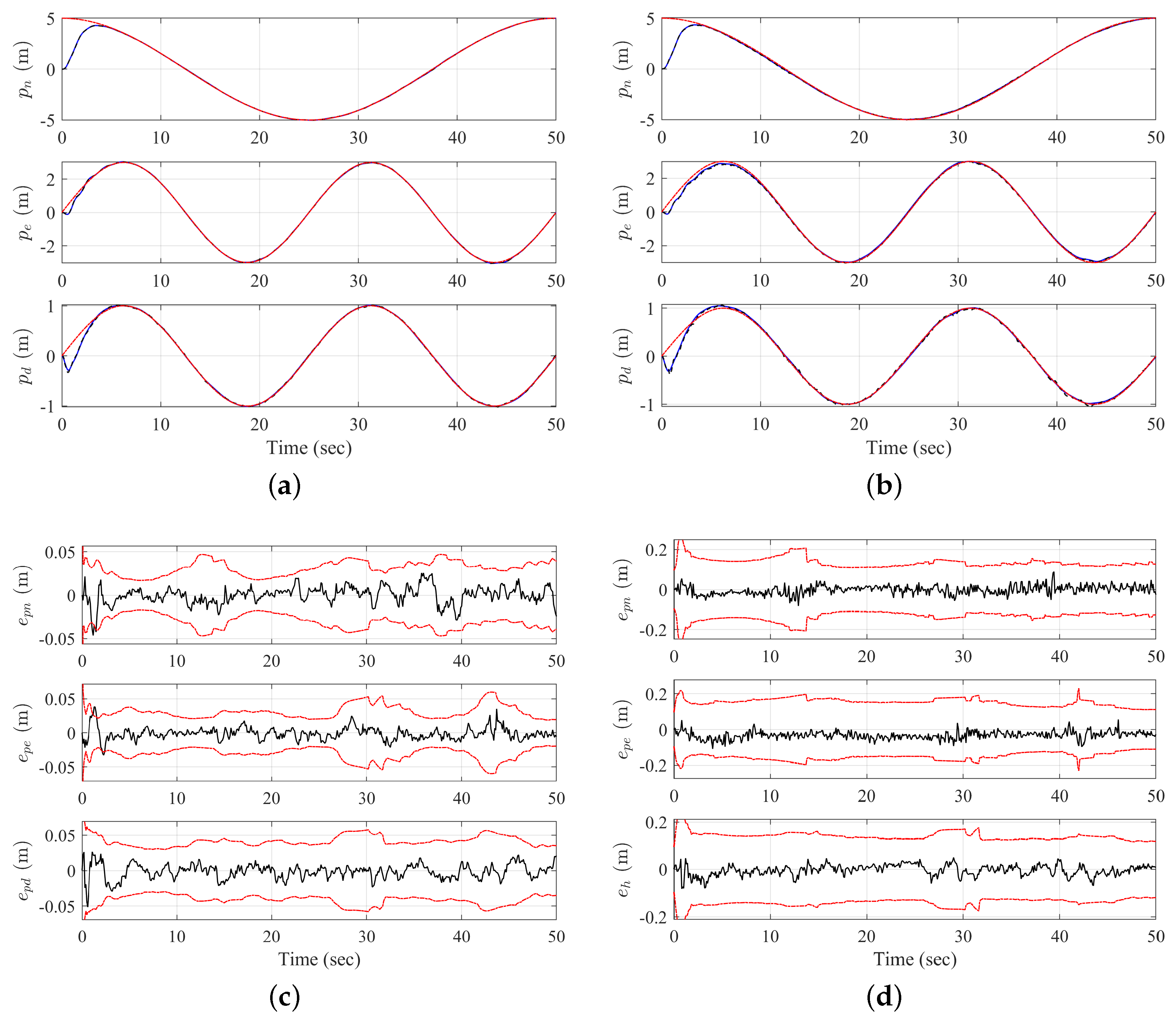
Figure 7 shows the results of the quadcopter traversing through an 8-shape trajectory using DF-LQR for the two scenarios considered for reviewing the effectiveness of EKF-SLAM. The first scenario is where the landmarks are known, i.e., their inertial positions are known and are used to make the updates during the localization of the quadcopter using EKF. This scenario does not include mapping as the landmarks are already known. The second scenario is where the mapping part of EKF-SLAM comes into effect as the landmarks are unknown. The positions of the landmarks are estimated relative to the initially assumed position of the quadcopter. It can easily be seen from the figure that the case of known landmarks has smoother trajectory control than the unknown case, which is expected.

3.1. Estimated Quadcopter States

Now, one compares the estimated states and errors for each of the scenarios to verify the effectiveness of EKF-SLAM using DF-LQR.
The initial state covariance ( P 0 ) and process noise covariance (Q) matrices considered for each of the scenarios are given in Table 6 and Table 7, respectively.
The estimated inertial position of the quadcopter for the known and unknown scenarios are plotted in Figure 8a,b, respectively. It is visible that the estimated positions are closer to the true trajectory in the known landmarks scenario than in the unknown landmarks scenario. It is more evident from the 3 σ boundaries for each scenario in Figure 8c,d, where the estimation error is lower for the known landmarks case than the unknown landmarks case. However, this greater error in the unknown landmarks scenario is inevitable considering the process also includes the estimation of landmark positions. Moreover, the average Root-Mean-Square Error (RMSE) over the duration of the simulation for its estimated inertial position hovered around 0.04 m when the landmarks were unknown compared to 0.012 m when the landmarks were known. Thus, the increase in the margin of error for the unknown landmarks case is not substantially larger than for the known landmarks case.
The same was the case when comparing results for the estimated velocities over the simulation duration of the two scenarios. As expected, when the landmarks were known, the quadcopter motion closely followed the desired velocity trajectory compared to when landmarks were unknown, as evident from Figure 9. The average RMSE for the estimated velocity of the quadcopter when landmarks were known was 0.03 m/s and that for unknown landmarks scenario was 0.04 m/s. Again, the estimations were accurate and not that far apart for the two scenarios. It was actually more erred for the known landmarks scenario, which is due to assumed P 0 and Q matrices.
The results for attitude estimations were astoundingly much better compared to other states estimated for the quadcopter as shown in Figure 10. The average RMSE for estimation of Euler angles during the simulation was just 0.34 deg for even the unknown landmarks case quite comparable to the known landmarks case, which hovered around 0.17 deg.
It should also be noted that the RMSE for each of the estimated states includes the initial high fluctuations before converging to the trajectory. This is mainly a result of the quadcopter’s initial position being at the origin, which is further from the initial desired trajectory position. It results in rapid motion of the quadcopter to reach the initial desired position and thus the higher fluctuations. Considering the motion of the quadcopter mainly when it has converged to its desired trajectory, the average RMSE is slightly lower for both the known and unknown landmark scenarios.

3.2. Estimation of Landmarks

The landmarks’ inertial position errors are estimated using EKF-SLAM and are depicted in Figure 11. Figure 11a shows that each of the inertial coordinates for each of the landmarks is estimated within the 3 σ boundary. It is visible in the figure that some landmarks are initialized after some time because they were sensed at that instant only. Thereafter, with the knowledge of uncertainties for previously identified and estimated landmarks, the uncertainty for newly discovered landmarks decreases over time. Figure 11b shows the final state of estimation error for all the landmarks at the end of the simulation. It can be seen that a few landmarks were never sensed and thus not initialized for estimation. The average RMSE for the estimated position for landmarks was around 0.03 m.

3.3. Computational Time Analysis for EKF-SLAM

The computational complexity of EKF-SLAM increases quadratically with the number of landmarks [7]. For a different number of landmarks ranging from 5 to 200, the averaged computational time for each of the major steps of EKF-SLAM is displayed in Figure 12. The prediction step of EKF is directly correlated to the number of mapped landmarks as the size of the cross-covariance matrix propagated in Equation (29) increases with it. Thus, the averaged computational time for the prediction step is seen varying quadratically with respect to the number of mapped landmarks in Figure 12a. Likewise, the computation time for the update depends on the number of landmarks that are observed and mapped. The linear trend of averaged computational time for the update considered with respect to the observed mapped landmarks is shown in Figure 12b, as the update step considers observed mapped landmarks. Lastly, the registration time in SLAM is also linearly dependent on the number of newly discovered landmarks that are registered as depicted in Figure 12c. It is evident from the figures that the computational effort of EKF-SLAM certainly increases quadratically with the number of landmarks. However, the main idea for generating these plots is to develop a metric or a strategy to run EKF-SLAM in real-time with a choice of the appropriate number of landmarks at each step, minimally affecting the total performance.
For instance, for better performance of EKF-SLAM, it is ideal not to miss any sensor data. Thus, considering the sensors’ sampling rate of 10 Hz, the steps of EKF-SLAM should ideally be complete within 0.1 s. Hence, if for example, the registration step is taking almost 0.1 s, it can be strategically decided to consider a finite number of landmarks using Figure 12c. Similarly, in case the update step itself is taking longer with making updates using all the observed mapped landmarks, only a few of those landmarks can be used to limit the time of operation to less than 0.1 s. Additionally, it is clear from Figure 12 that the update and registration steps take more time than the prediction step. Additionally, only after 200 mapped landmarks does prediction have a significant effect on computation time. Hence, if a mission identifies less than around 200 landmarks, decisions can be based upon choosing an appropriate number of landmarks for update and registration. However, in case the number of mapped landmarks is more, decisions can be made where only a few landmarks at random are taken into consideration during the prediction step. It should be noted the results in Figure 12 will vary among different computers. The results shown were generated using a computer with Intel i7-11800H 2.30 GHz processor, 16 GB RAM, and an NVIDIA T1200 GPU 4 GB. However, these sets of plots will be similar and can be used to make decisions on the number of landmarks to consider for each step of EKF-SLAM to improve its real-time performance.

4. Conclusions

This work proposes an Extended Kalman Filter-based Simultaneous Localization And Mapping (EKF-SLAM) for a quadcopter to follow aggressive trajectories using a Differential Flatness-based Linear Quadratic Regulator (DF-LQR). A strategy to reduce the computational effort of EKF-SLAM using averaged computational time of operation for each step of the process with respect to the number of landmarks is also proposed in the end. To validate the performance of the proposed approach, the quadcopter traversing an 8-shape trajectory is considered for two scenarios of known landmarks and unknown landmarks, and to imitate practical conditions, sensors’ constraints, such as limited sensing ranges and field of views, are considered. The estimation errors for the quadcopter states are comparable for both cases despite the lack of information on the landmarks in the unknown landmarks scenario. When following the given trajectory, the estimated states of both the quadcopter and landmarks are accurate enough for DF-LQR to generate the appropriate control signal using the estimated states themselves. The estimated position, velocity, and attitude of the quadcopter are extremely accurate along with the estimation of the landmark positions evident from extremely low root-mean-square errors. The computation time analysis for each step of EKF-SLAM with respect to the number of landmarks shows that the computational time does increase quadratically with the number of landmarks, and the results are identified to be beneficial in strategically choosing the respective number of landmarks for each step to maximize the use of sensor data and improve performance. Albeit this work validates the proposed approach via numerical simulations, hardware experiments will be conducted to verify its real-time applicability during the quadcopter’s aggressive maneuvers in future work.

Author Contributions

Conceptualization, S.R. and S.B.; methodology, S.R., S.B., D.C. and D.K.; software, S.R. and S.B.; validation, S.R., S.B. and D.C.; formal analysis, S.R., S.B., D.C. and D.K.; investigation, S.R. and S.B.; resources, D.K.; data curation, S.R. and S.B.; writing—original draft preparation, S.R. and S.B; writing—review and editing, D.C. and D.K.; visualization, S.R., S.B. and D.C.; supervision, D.K.; project administration, D.K.; funding acquisition, D.K. All authors have read and agreed to the published version of the manuscript.

Funding

This research received no external funding.

Data Availability Statement

Not applicable.

Conflicts of Interest

The authors declare no conflict of interest.

References

  1. Cadena, C.; Carlone, L.; Carrillo, H.; Latif, Y.; Scaramuzza, D.; Neira, J.; Reid, I.; Leonard, J.J. Past, present, and future of simultaneous localization and mapping: Toward the robust-perception age. IEEE Trans. Robot. 2016, 32, 1309–1332. [Google Scholar] [CrossRef] [Green Version]
  2. Sadeghzadeh-Nokhodberiz, N.; Can, A.; Stolkin, R.; Montazeri, A. Dynamics-based modified fast simultaneous localization and mapping for unmanned aerial vehicles with joint inertial sensor bias and drift estimation. IEEE Access 2021, 9, 120247–120260. [Google Scholar] [CrossRef]
  3. Suzuki, T.; Amano, Y.; Hashizume, T. Development of a SIFT based monocular EKF-SLAM algorithm for a small unmanned aerial vehicle. In Proceedings of the SICE Annual Conference 2011, Tokyo, Japan, 13–18 September 2011; pp. 1656–1659. [Google Scholar]
  4. Karam, S.; Nex, F.; Chidura, B.T.; Kerle, N. Microdrone-Based Indoor Mapping with Graph SLAM. Drones 2022, 6, 352. [Google Scholar] [CrossRef]
  5. Balamurugan, G.; Valarmathi, J.; Naidu, V. Survey on UAV navigation in GPS denied environments. In Proceedings of the 2016 International Conference on Signal Processing, Communication, Power and Embedded System (SCOPES), Paralakhemundi, India, 3–5 October 2016; pp. 198–204. [Google Scholar]
  6. Smith, R.; Self, M.; Cheeseman, P. Estimating uncertain spatial relationships in robotics. In Autonomous Robot Vehicles; Springer: New York, NY, USA, 1990; pp. 167–193. [Google Scholar]
  7. Durrant-Whyte, H.; Bailey, T. Simultaneous localization and mapping: Part I. IEEE Robot. Autom. Mag. 2006, 13, 99–110. [Google Scholar] [CrossRef] [Green Version]
  8. Takleh, T.T.O.; Bakar, N.A.; Rahman, S.A.; Hamzah, R.; Aziz, Z. A brief survey on SLAM methods in autonomous vehicle. Int. J. Eng. Technol. 2018, 7, 38–43. [Google Scholar] [CrossRef] [Green Version]
  9. Cho, Y.; Hwang, J.Y. A study on EKF-SLAM simulation of autonomous flight control of quadcopter. Int. J. Softw. Eng. Its Appl. 2015, 9, 269–282. [Google Scholar] [CrossRef]
  10. Azizi, A.; Nourisola, H.; Ghiasi, A.R. 3D inertial algorithm of SLAM for using on UAV. In Proceedings of the 2016 4th International Conference on Robotics and Mechatronics (ICROM), Tehran, Iran, 26–28 October 2016; pp. 122–129. [Google Scholar]
  11. Hening, S.; Ippolito, C.A.; Krishnakumar, K.S.; Stepanyan, V.; Teodorescu, M. 3D LiDAR SLAM integration with GPS/INS for UAVs in urban GPS-degraded environments. In Proceedings of the AIAA Information Systems-AIAA Infotech@ Aerospace, Grapevine, TX, USA, 9–13 January 2017; p. 0448. [Google Scholar]
  12. Kim, H.; Kim, D.; Kim, S. Real-time Geospatial Positioning for UAVs in GPS-Denied Environment Using LiDAR Data. In Proceedings of the AIAA Scitech 2020 Forum, Orlando, FL, USA, 6–10 January 2020; p. 2194. [Google Scholar]
  13. Yu, W.; Zamora, E. Sliding mode three-dimension SLAM with application to quadrotor helicopter. In Proceedings of the 2018 15th International Conference on Electrical Engineering, Computing Science and Automatic Control (CCE), Mexico City, Mexico, 5–7 September 2018; pp. 1–6. [Google Scholar]
  14. Bagheri, S.; Jafarov, T.; Freidovich, L.; Sepehri, N. Beneficially combining LQR and PID to control longitudinal dynamics of a SmartFly UAV. In Proceedings of the 2016 IEEE 7th Annual Information Technology, Electronics and Mobile Communication Conference (IEMCON), Vancouver, BC, Canada, 13–15 October 2016; pp. 1–6. [Google Scholar]
  15. Ferrin, J.; Leishman, R.; Beard, R.; McLain, T. Differential flatness based control of a rotorcraft for aggressive maneuvers. In Proceedings of the 2011 IEEE/RSJ International Conference on Intelligent Robots and Systems, San Francisco, CA, USA, 25–30 September 2011; pp. 2688–2693. [Google Scholar]
  16. Paz, L.M.; Tardós, J.D.; Neira, J. Divide and conquer: EKF SLAM in o(n). IEEE Trans. Robot. 2008, 24, 1107–1120. [Google Scholar] [CrossRef]
  17. Beard, R.W. Quadrotor dynamics and control. Brigh. Young Univ. 2008, 19, 46–56. [Google Scholar]
  18. Luukkonen, T. Modelling and control of quadcopter. Indep. Res. Proj. Appl. Math. Espoo 2011, 22, 22. [Google Scholar]
  19. Martins, L.; Cardeira, C.; Oliveira, P. Linear quadratic regulator for trajectory tracking of a quadrotor. IFAC-PapersOnLine 2019, 52, 176–181. [Google Scholar] [CrossRef]
  20. Rigatos, G.G. Differential flatness theory and flatness-based control. In Nonlinear Control and Filtering Using Differential Flatness Approaches; Springer: Cham, Switzerland, 2015; pp. 47–101. [Google Scholar]
  21. Tedrake, R. Underactuated robotics: Learning, planning, and control for efficient and agile machines course notes for MIT 6.832. Work. Draft. Ed. 2009, 3, 91–92. [Google Scholar]
  22. Hespanha, J.P. Linear Systems Theory; Princeton University Press: Princeton, NJ, USA, 2018. [Google Scholar]
  23. Saraf, P.; Gupta, M.; Parimi, A.M. A Comparative Study Between a Classical and Optimal Controller for a Quadrotor. In Proceedings of the 2020 IEEE 17th India Council International Conference (INDICON), New Delhi, India, 10–13 December 2020; pp. 1–6. [Google Scholar]
  24. Leishman, R.C.; Macdonald, J.C.; Beard, R.W.; McLain, T.W. Quadrotors and accelerometers: State estimation with an improved dynamic model. IEEE Control. Syst. Mag. 2014, 34, 28–41. [Google Scholar]
  25. Sola, J. Simultaneous localization and mapping with the extended Kalman filter. Oct 2014, 5, 35. [Google Scholar]
  26. Bailey, T.; Durrant-Whyte, H. Simultaneous localization and mapping (SLAM): Part II. IEEE Robot. Autom. Mag. 2006, 13, 108–117. [Google Scholar] [CrossRef] [Green Version]
Figure 1. Definitions of the reference frames and the state variables of the quadcopter.
Electronics 12 01113 g001
Figure 2. Flowchart of the trajectory control.
Electronics 12 01113 g002
Figure 3. Classification of landmarks.
Electronics 12 01113 g003
Figure 4. EKF-SLAM flowchart in the sensing, navigation, and control system.
Electronics 12 01113 g004
Figure 5. Spherical coordinate representation of LiDAR measurement of a landmark.
Electronics 12 01113 g005
Figure 6. (a) Error covariance matrix at the beginning of the i th time step, (b) predicted covariance matrix, (c) updated part of the covariance matrix, and (d) augmented covariance matrix with a single new landmark. Shaded regions are where changes happen. Dark gray represents respective covariance and pale gray represents cross-variance.
Electronics 12 01113 g006
Figure 7. Quadcopter traversing 8-shape trajectory for different scenarios. (a) Known landmarks. (b) Unknown landmarks.
Electronics 12 01113 g007
Figure 8. Quadcopter’s estimated position and corresponding estimation error when following an 8-shape trajectory for different cases. For (a) position for known landmarks and (b) position for unknown landmarks, true states (──), estimated states (Electronics 12 01113 i002), and desired states (Electronics 12 01113 i001). For (c) estimated position error for known landmarks and (d) estimated position error for unknown landmarks, estimation error (──), and 3 σ boundary (Electronics 12 01113 i001).
Electronics 12 01113 g008
Figure 9. Quadcopter’s estimated velocity and corresponding estimation error when following an 8-shape trajectory for different cases. For (a) position for known landmarks and (b) position for unknown landmarks, true states (──), estimated states (Electronics 12 01113 i002), and desired states (Electronics 12 01113 i001). For (c) estimated position error for known landmarks and (d) estimated position error for unknown landmarks, estimation error (──), and 3 σ boundary (Electronics 12 01113 i001).
Electronics 12 01113 g009
Figure 10. Quadcopter’s estimated Euler angles and corresponding estimation error when following an 8-shape trajectory for different cases. For (a) attitude for known landmarks and (b) attitude for unknown landmarks, true states (──), estimated states (Electronics 12 01113 i002), and desired states (Electronics 12 01113 i001). For (c) estimated attitude error for known landmarks and (d) estimated attitude error for unknown landmarks, estimation error (──), and 3 σ boundary (Electronics 12 01113 i001).
Electronics 12 01113 g010
Figure 11. Landmarks state estimation error for an 8-shape trajectory. For Figure 11a, estimation error (──), 3σ boundary (Electronics 12 01113 i001); each line signifying estimation error for each landmark over time. (a) Estimation error over time and (b) estimation error at the end.
Electronics 12 01113 g011
Figure 12. Computational time for different steps of EKF-SLAM with respect to the number of landmarks. (a) Computational time of prediction step vs. number of mapped landmarks, (b) computational time of update step vs. number of observed mapped landmarks, and (c) computational time of registration step vs. number of observed unmapped landmarks.
Electronics 12 01113 g012
Table 1. Quadcopter properties.
ParameterValue
Mass, m1.56 kg
Inertia matrix, J diag 0.114700 , 0.057600 , 0.171200 kg-m 2
Table 2. LQR weight matrices.
ParameterValue
Q ˜ diag 0.01 , 0.01 , 0.01 , 0.01 , 0.01 , 0.01 , 0.04
R ˜ diag 0.2 , 0.32 , 0.1
Table 3. Landmark region specifications.
ParameterValue
Number of landmarks, n40
Azimuth 180 , 180 deg
Elevation 50 , 50 deg
Range 8 , 20 m
Table 4. LiDAR sensor specifications.
ParameterValue
Azimuth ( α ) FOV 45 , 45 deg
Elevation ( β ) FOV 30 , 30 deg
Range ( δ ) 0 , 100 m
Azimuth noise, σ α 0.33 deg
Elevation noise, σ β 0.3 deg
Radial noise, σ δ 0.1 m
Sampling rate10 Hz
Table 5. IMU sensor specifications.
ParameterValue
Accelerometer (ND)300 μ g / rtHz 2
Gyroscope (ND)0.01 ( deg / s ) / rtHz
Sampling rate10 Hz
Table 6. Initial state covariance and process noise covariance matrices for the known landmarks scenario.
ParameterValue
Initial state covariance ( P 0 ) diag 0.01 , 0.01 , 0.01 , 0.01 , 0.01 , 0.01 , 0.02 , 0.02 , 0.02
Process noise covariance (Q) diag 0.01 , 0.01 , 0.01 , 0.01 , 0.01 , 0.01 , 0.02 , 0.02 , 0.02
Table 7. Initial state covariance and process noise covariance matrices for the unknown landmarks scenario.
ParameterValue
Initial state covariance ( P 0 ) diag 0.001 , 0.001 , 0.001 , 0.1 , 0.1 , 0.1 , 0 , 0 , 0
Process noise covariance (Q) diag 0.2 , 0.2 , 0.05 , 0.01 , 0.01 , 0.01 , 0.02 , 0.2 , 0.2
Disclaimer/Publisher’s Note: The statements, opinions and data contained in all publications are solely those of the individual author(s) and contributor(s) and not of MDPI and/or the editor(s). MDPI and/or the editor(s) disclaim responsibility for any injury to people or property resulting from any ideas, methods, instructions or products referred to in the content.

