Optimal Transport-Embedded Neural Network for Fairness Transfer Problem

Abstract

Research on neuromorphic computing has gained popularity in recent years. In particular, regularized embedded neural systems have been applied in several significant real-world situations, such as recommendation systems and transfer learning. This paper deals with the fairness transfer learning problem, which has been insufficiently explored. In fairness transfer settings, the source domain has limit-tagged training samples, which may lead to performance degradation in the target domain. To solve such problems, a linear data-augmentation-based optimal transport-embedded neural network is proposed in this paper. It can augment the source samples to make the distribution of the source domain balanced and can align the source and target distributions simultaneously. Moreover, the distribution of the augmented data by mixup is limited to a certain bound that can avoid the abnormal samples generated. The effectiveness of the proposed method has been demonstrated in several transfer learning tests, including regression and classification. In 1-shot and 3-shot classification tasks on the Office dataset, our method’s accuracy is 4.8 and 3.9% better, respectively, than the second-best model. Additionally, our model’s performance is about 2–3 percentage points superior to the second-best model in the OfficeHome dataset. It is simple yet effective, making it perfect for low-power edge AI applications.

1. Introduction

Neural network-based methods have achieved significant advances in building decision algorithms and have been applied in various real-world applications. They have been used widely in some sensitive areas that usually possess a large number of samples, such as control, classification, prediction, and other tasks [1,2]. Machine-learning methods are good at mining increasingly abstract distributed feature representations from original input data, and these representations have good generalization ability. However, the performance of machine-learning methods relies heavily on the quality and the number of training samples. The decision rule learns on the training set and is applied on the test set under the assumption that the training and the test samples from different domains follow the same underlying distribution [3]. The optimization of most machine-learning methods breaks down in the small-data regime, where only very few labeled examples are available for training. This indicates that the decision boundary of the learned model is highly influenced by the training set.

The availability of massive data with fully labeled information is crucial since data collection and annotation are very expensive and time-consuming for some specific objects. This has motivated researchers to produce novel algorithms or learning models that are trained with few examples (or only one example) and have ideal performance on the test set. In the past decade, few-shot learning has attracted much researcher interest, which is a type of machine-learning problem where the training dataset contains limited information. Many few-shot learning methods are proposed to solve such problems, and they can be subdivided into two broad categories: data-augmentation methods and meta-learning methods [4]. The former is usually based on the Generative Adversarial Network (GAN), which focuses on synthesizing the training data using some specific conditions. GANs contain two sub-networks: a generator and a discriminator. The generator creates samples to deceive the discriminator, while the discriminator determines if a sample is created or real [5]. The latter is based on an episodic training strategy that uses a few examples of each episode from the base class set to mimic the test scenario.

Traditional machine-learning problems assume that the feature space and data distribution of the training set and the test set are the same. In some real applications, samples from specific domains are expensive and difficult to collect. Thus, it is of significant importance to create a high-performance learning model trained with data from easily obtained domains. This methodology is referred to as transfer learning and has been widely studied. It aims to reduce the marginal mismatch in feature space between different domains and transfer information from well-labeled source domain samples to unlabeled target samples. The existing transfer learning models can be categorized into two groups: discrepancy-based methods and GAN-based methods [6]. However, they are all based on the concept of reducing cross-domain gaps by aligning the domain distribution so that models derived from the source domain can be applied directly to the target domain. Inspired by the dynamic control theory [7], more and more machine-learning methods have focused on developing a model that can be explained. In this paper, we propose an optimal transport model that can be theoretically analyzed.

For optimal transport problems, this is the most effective method to perform the transformation of one mass distribution into another mass distribution. The basic types of these problems include the Monge transmission problem, Kantorovich transmission problem, and Kantorovich dual transmission problem [8]. At present, the optimal transmission problem has been applied to many fields, such as transfer learning [9,10], image processing [11], sequence pattern analysis [12], and so on. Courty et al. [13] assumed that there was a nonlinear transformation between the joint distribution of the source domain and the target domain, which could be estimated using the optimal transport method, and proposed a solution model named JDOT to recover the estimated target distribution by optimizing the coupling matrix and classifier simultaneously. On this basis, Damodaran et al. [14] proposed a new deep-learning framework, DeepJDOT, to obtain better classification results through a neural network model.

In this paper, a novel optimal transport-based neural system is proposed to solve the fairness transfer learning problem. Imbalanced or long-tailed distributions are quite normal in real-world scenarios, and transfer learning is much more difficult to solve than in traditional machine-learning settings. Thus, fairness transfer learning is a more challenging and piratical task for imbalanced data, as is commonly encountered in real-world applications. It aims to learn a classifier from only a few examples in the source domain and transfer the knowledge to a novel target domain [15,16]. This paradigm is pretty similar to human behaviors that transfer learned experience to new tasks. This occurs instead of adapting a Generative Adversarial Network to augment the samples from the few-shot source samples. Our proposed method aims to solve the fairness transfer learning problem with a linear data-augmentation-based optimal transport model. It is much easier in the training process and can constrain the distribution of augmented data in a certain bound. Optimal transport-embedded neural systems are an option for solving transfer learning problems. The mixup method is adopted in this paper. It trains the optimal transport model with convex combinations of pairs of examples and their labels. In addition, the conditional distributions of the mixup source domain and target domain are aligned by the optimal transport model. The learning model and the coupling matrix for distribution alignment are optimized simultaneously. Some synthetic examples and widely used transfer learning tasks demonstrate the efficiency of the proposed model, and the theoretic analysis is provided.

The rest of this paper is organized as follows. Section 2 provides the preliminaries. Section 3 reformulates the proposed equivalent problem with the mixup augmentation mechanism, and derives closed-form solutions via the stochastic gradient descent method, and theoretic analysis is provided. Section 4 exhibits a series of experimental results. Finally, Section 5 concludes this paper.

2. Definitions of Fairness Transfer Learning

A domain $\mathcal{D}$ is defined with a feature space $\mathcal{X}$ and the corresponding marginal distribution $P\left(X\right)$, where $X=[x_1,x_2,\dots ,x_n]\in \mathcal{X}$, n is the number of training samples. The learning task $\mathcal{T}$ on the domain $\mathcal{D}$ is to learn a classifier f that can project the features $X\in \mathcal{X}$ to the corresponding labels $Y\in \mathcal{Y}$. As for transfer learning, given a source domain ${\mathcal{D}}_S=\{(x_{s_1},y_{s_1}),(x_{s_2},y_{s_2}),\dots ,(x_{s_n},y_{s_n})\}$ and a target domain ${\mathcal{D}}_T=\{(x_{t_1},y_{t_1}),(x_{t_2},y_{t_2}),\dots ,(x_{t_n},y_{t_n})\}$, where the two margin distributions are different, $P\left(X_S\right)\ne P\left(X_T\right)$. Usually in transfer learning $\{X_s\in {\mathcal{D}}_S\}\ne \{X_t\in {\mathcal{D}}_T\}$, but $Y_s$ and $Y_t$ share the same class information. If ${\mathcal{D}}_S={\mathcal{D}}_T$, the problem becomes a traditional machine-learning problem.

The corresponding tasks of the two domains are denoted as ${\mathcal{T}}_S$ and ${\mathcal{T}}_T$. It has been demonstrated that a classifier trained with the samples from the source domain will not perform optimally on the target domain if the two marginal distributions are different [17]. Therefore, the goal of transfer learning is to improve the transferability and generalization of the classifier in task ${\mathcal{T}}_T$ using the knowledge from the source domain set ${\mathcal{D}}_S$ and the task ${\mathcal{T}}_S$.

In the fairness learning scenario, the alignment and the separation of probability distributions are difficult due to the lack of training data. The fairness transfer learning setting can be divided into two categories. One class is with sufficient well-labeled samples in the source domain and a few labeled samples in the target domain. Some work has been done to solve such a problem [18,19]. Most of them focus on extending adversarial learning to exploit the label information of target samples. The other class is the fairness source domain transfer learning problem, which is more challenging than the first class, for it aims to classify the unlabeled target samples with a few labeled source samples. Little work has been done for transfer learning under such fairness settings.

In this paper, we study the problem of fairness source domain transfer learning and define the settings as follows.

Assume the training samples in the source domain can be categorized into two sub-sets: the minority set ${\mathcal{D}}_S^m$ (the classes with limit samples) and the default set ${\mathcal{D}}_S^d$ (the classes with sufficient samples). The minority set and the default set have no visual features or class information overlapped. In addition, we want to train a classifier f on the imbalanced source domain and generalize the f to have a good performance on the unlabeled target domain. If the average loss of minority classes and the default classes are directly used to train the classifier, that may lead to bias towards default classes and unsatisfied classification results on the minority classes.

Denote the joint distributions probability over features X and domain ${\mathcal{D}}_S^m/{\mathcal{D}}_S^d$ of the classifier f as $\mathbb{P}(f\left(X_S^m\right)=\mathrm{True}|{\mathcal{D}}_{\mathrm{S}}^{\mathrm{m}})$ and $\mathbb{P}(f\left(X_S^d\right)=\mathrm{True}|{\mathcal{D}}_{\mathrm{S}}^{\mathrm{d}})$, respectively. The $(f(·)=\mathrm{True}|{\mathcal{D}}_{\mathrm{S}}^{\mathrm{i}})$, denotes the correctly classified samples in the specific source sub-domain, where $i=\{{\mathcal{D}}_S^m,{\mathcal{D}}_S^d\}$. Then the balanced error rate with respect to the joint distribution of the feature X can be defined as follows

$$\begin{array}{c}\hfill BER(f,X,{\mathcal{D}}_S)=\frac{\mathbb{P}(f\left(X\right)=\mathrm{True}|{\mathcal{D}}_{\mathrm{S}}^{\mathrm{m}})+1-\mathbb{P}(\mathrm{f}\left(\mathrm{X}\right)=\mathrm{True}|{\mathcal{D}}_{\mathrm{S}}^{\mathrm{d}})}{2}\hfill \end{array}$$

where $BER(f,X,{\mathcal{D}}_S)$ is the misclassification error of f when the classes of the fairness domain and default domain are equally like, i.e., $\mathbb{P}\left({\mathcal{D}}_S^m\right)=\mathbb{P}\left({\mathcal{D}}_S^d\right)=1/2$, which means the probability of correctly classified results is the same across the groups. And according to [20], the classifier f has disparate impact at level $\tau$, if and only if

$$\begin{array}{c}\hfill BER(f,X,{\mathcal{D}}_S)\le \frac{1}{2}-\frac{\mathbb{P}(f\left(X\right)=\mathrm{True}|{\mathcal{D}}_{\mathrm{S}}^{\mathrm{m}})}{2}(\frac{1}{\tau }-1).\hfill \end{array}$$

That indicates that, in principle, we can modify the classifier or the input data to eliminate possible classifier-related differences.

3. Linear Data Augmentation Based Optimal Transport Model

To tackle the problem mentioned above, we focus on changing the data distribution of the fairness source domain to ensure the classifier trained from the modified source domain would be fair overall classes.

First, we introduce the baseline of the proposed model. The optimal transport problem is to seek a transformation $\mathcal{T}$ that aligns source distribution $P\left(X_S\right)$ to target distribution $P\left(X_T\right)$, defined as follows

$$\begin{array}{cc}\hfill {\mathcal{T}}_0=& arg\underset{T}{min}\int d(x,\mathcal{T}\left(x\right))dP\left(X_S\right)\left(x\right),\hfill \\ \hfill \mathrm{s}.\mathrm{t}.& \mathcal{T}†P\left(X_S\right)=P\left(X_T\right),\hfill \end{array}$$

(1)

where $\mathcal{T}†P\left(X_S\right)$ is the image map of $P\left(X_S\right)$ to $P\left(X_T\right)$ by $\mathcal{T}$. When ${\mathcal{T}}_0$ exists, it is called an optimal transport map.

Then the original optimal transport problem (1) can be relaxed to Kantorovitch problem [21], which aims to find a transport plan over the two distributions

$$\begin{array}{c}\hfill {\gamma }_0=arg\underset{\gamma }{min}\int d(x_1,x_2)d\gamma (x_1,x_2),\hfill \end{array}$$

(2)

where $\gamma \in \prod (P\left(X_S\right),P\left(X_T\right))$, and $\prod (P\left(X_S\right),P\left(X_T\right))=\left\{\gamma \right|p^{+}†\gamma =P\left(X_S\right),p^{-}†\gamma =P\left(X_T\right)\}$, $p^{+}$ and $p^{-}$ are the two marginal projections of the joint distributions.

As mentioned in [13], the changes in marginal and conditional distributions are all taken into consideration. It seeks a map $\mathcal{T}$ that can align the joint distributions of source and target domains. Following the Kantovorich formulation, then we have

$$\begin{array}{c}\hfill {\gamma }_0=arg\underset{\gamma }{min}\int D(x_i,y_i;x_j,y_j)d\gamma (x_i,y_i;x_j,y_j),\hfill \end{array}$$

(3)

where $D(x_i,y_i;x_j,y_j)=d(x_i,x_j)+\mathcal{L}(y_i,y_j)$ which calculates the distances of the features and the discrepancy of the labels. $(x_i,y_i)$ is the sample from the source domain and $(x_j,y_j)$ the sample from the target domain. The label information $y_j$ of the target sample is unknown, but it can be obtained by the classifier $y_j=f\left(x_i\right)$.

Our goal is to train a classifier f from the source domain that can perform well on the target domain, which can optimally match the labels of source domain samples with the features of the target domain in the transport plan. Thus, the joint distribution optimal transport problem in discrete form can be formulated as

$$\begin{array}{c}\hfill \underset{\gamma }{min}\sum _{i,j}D(x_i,y_i;x_j,y_j){\gamma }_{ij}.\hfill \end{array}$$

(4)

Additionally, a regularization term is added to the classifier, and f is to be updated while learning the optimal coupling matrix $\gamma$:

$$\begin{array}{c}\hfill \underset{\gamma ,f}{min}\sum _{i,j}{\gamma }_{ij}(d(x_i,x_j)+\mathcal{L}(y_i,f\left(x_j\right))+\delta \Omega \left(f\right),\hfill \end{array}$$

(5)

where $\Omega$ is the constraint on f, and $\mathcal{L}$ is continuous and differentiable with respect to its second variable. $\delta$ is the trade-off parameter.

To tackle the fairness transfer learning problem, most methods utilize GANs to augment the samples to have a balanced data distribution. However, there is a more simple and efficient method proposed for linear data augmentation, named mixup [22]. The mixup is to pair similar samples in the training set, formalized by the Vicinal Risk Minimization principle. It assumes that the examples in the vicinity share the label information and does not model proximity in different classes of examples. Mixup interpolates the training samples as follows

$$\begin{array}{cc}\hfill x_m^s=\hfill & \hfill \lambda x_i^s+(1-\lambda )x_j^s,\hfill \\ \hfill y_m^s=\hfill & \hfill \lambda y_i^s+(1-\lambda )y_j^s,\hfill \end{array}$$

(6)

where $(x_i^s,y_i^s)$ and $(x_j^s,y_j^s)$ are the training samples randomly selected from the fairness source domain. The distributions of the two new sub-source domains are denoted as ${\mu }_1^s$ and ${\mu }_2^s$, respectively. The labels are usually set as one-hot labels, and $\lambda \in [0,1]$ is the mixup parameter. Mixup extends the source distribution by incorporating feature vectors. It can be simply implemented and introduces minimal computation overhead.

Based on the spirit of JDOT, which is formulated as Equation (5), we combine the mixup data obtained from Equation (6) with the optimal transport model, and the model becomes:

$$\begin{array}{c}\hfill \underset{\gamma ,f}{min}\sum _{i,j}{\gamma }_{ij}(d(x_i^m,x_j^t)+\mathcal{L}(y_i^m,y_j^t))+\delta \Omega \left(f\right),\hfill \end{array}$$

(7)

where $(x_i^m,y_i^m)$ and $(x_j^t,y_j^t)$ are the samples from the mixup source domain and the target domain, respectively. $\delta$ is the penalty parameter.

The parameters in (7) can be optimized alternatively. The optimization process of the proposed mixup optimal transport model for the fairness transfer learning problem is stated as follows:

Step 1: Given the fairness source samples, augment the data by Equation (6) and obtain the mixup source domain.

Step 2: Fix the parameters of f in Equation (7), optimize $\gamma$ with simplex flow algorithm.

Step 3: Fix the transformation matrix $\gamma$ in Equation (7) and update the parameters of f by stochastic gradient method.

Step 4: Check the convergence condition; if satisfied, end the optimization process.

Remark 1.

The mixup procedure randomly changes the distribution of the original source domain by selecting the sample pairs and doing the interpolation. The degree of mixup is dominated by the mixup parameter λ, which can imply the total variation distance of the two conditional distributions. According to [23], the total distance variation (TDV) of the two probabilities distributions $P_1,P_2$ can be calculated as

$$\begin{array}{c}\hfill d_{TDV}(P_1,P_2)=\underset{\pi \in \prod (P_1,P_2)}{min}\pi (x\ne y).\hfill \end{array}$$

Let M be the target variable in distribution ${\mu }_i^s$, where $s\in \{1,2\}$. ${\mathcal{T}}_i$ is the transformation that push each source distribution ${\mu }_i$ towards the target distribution ${\mu }_t$, i.e., $\mathcal{T}†{\mu }_i={\mu }_t$. Set ${\mathcal{R}}_i={\mathcal{T}}_i^{-1}$ and ${\mathcal{R}}_i\left(M\right)$ follows the original source distribution ${\mu }_s$. Then we have:

$$\begin{array}{cc}\hfill d_{TDV}({\mu }_1^s,{\mu }_2^s)\le & P(\lambda M+(1-\lambda ){\mathcal{R}}_1\left(M\right)\ne \lambda M+(1-\lambda ){\mathcal{R}}_2\left(M\right))\hfill \\ \hfill =& 1-P(\lambda M+(1-\lambda ){\mathcal{R}}_1\left(M\right)=\lambda M+(1-\lambda ){\mathcal{R}}_2\left(M\right))\hfill \\ \hfill \le & 1-\lambda .\hfill \end{array}$$

This bound ensures the distribution of the two mixup source domains is a constraint in a constraint. If $\lambda =0$, it leaves the original distributions unchanged.

4. Experiment

In the following experiments, we test the proposed method on regression tasks, simple toy classification tasks, digital transfer classification tasks, and object transfer classification tasks, respectively. For the fairness transfer learning problem in this paper, the ResNet-50 is utilized as the backbone of the proposed model. The optimal transport embedded neural network is trained using stochastic gradient descent (SGD) with a batch size of 32 and a learning rate of 0.001. The SGD optimizer uses a momentum of 0.9 and a weight decay of 0.001. The bottleneck dimension for the features is set to 2048. The $\delta$ is set as 1. The mixup parameter $\lambda$ follows the beta distribution $Beta(\alpha ,\alpha )$ and we set the $\alpha$ as 2.

4.1. Regression Examples

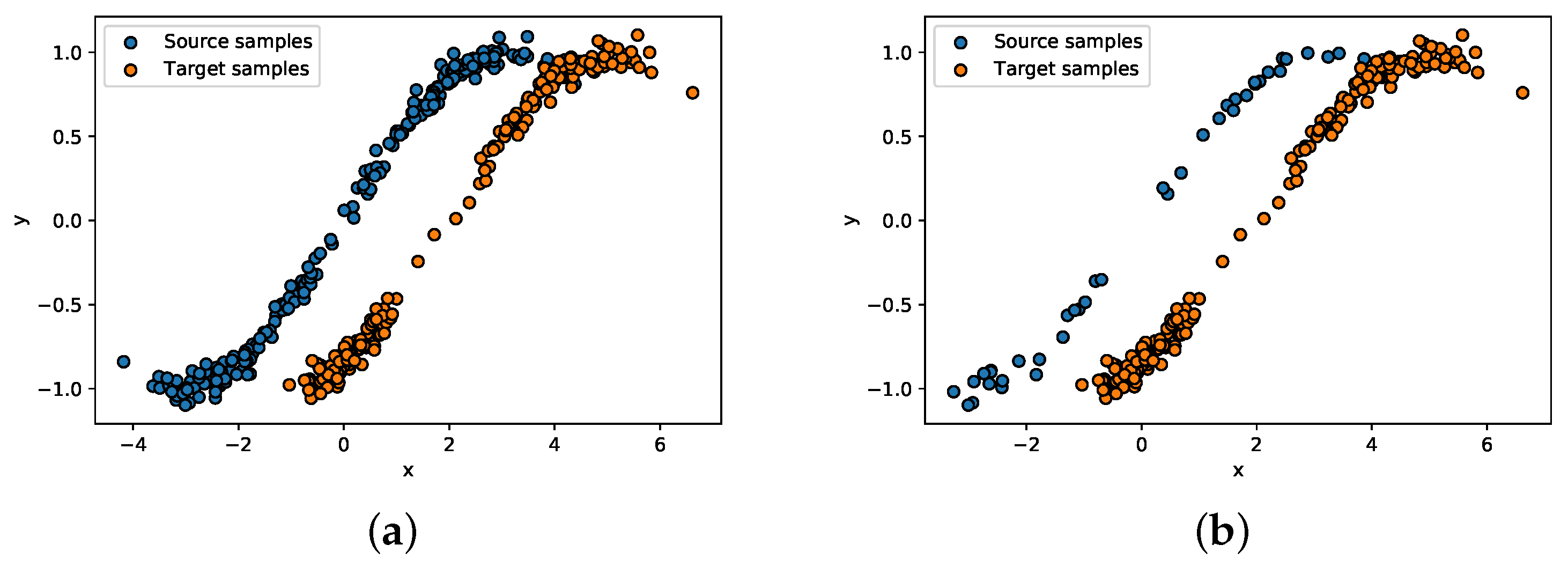
First, we test the proposed model in a simple transfer learning regression problem under the traditional settings that the source domain has sufficient samples for training. The distributions of the two domains are shown in Figure 1a. The blue dots are the source samples, and the orange dots are the target samples. Each domain obtains 200 samples. The two domains have a similar amplitude in y, but different distributions in x. The (x, y) in the figures represent the samples’ corresponding coordinates after embedding. If the regression model learned from the source domain is applied directly to the target domain, the result is not satisfactory. However, the regression model learned from the JDOT model can be generalized to the source domain and target domain as well. When it comes to fairness transfer learning settings, the number of training samples in the source domain is reduced from 200 to 40. The fairness data distributions and the learned models are demonstrated in Figure 1b.

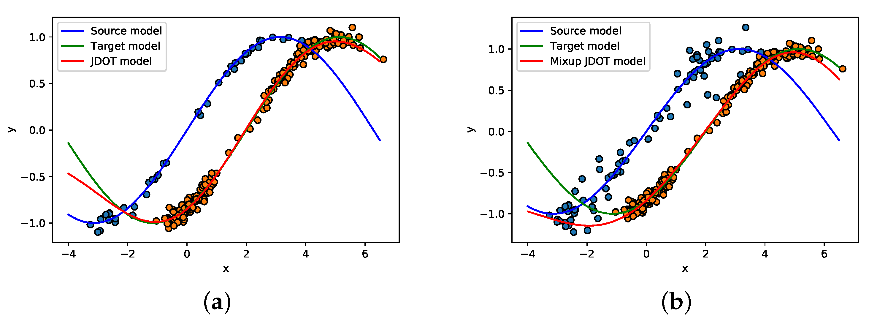
Then, we adapt the traditional optimal transport method JDOT and our proposed method MixupJDOT to the fairness transfer regression problem. First, we augment the source domain by mixup, randomly select the paired training samples, and obtain the new mixup samples by Equation (3). Then, we adapt our proposed method to the fairness transfer regression problem. Figure 2a presents the three regression models, the blue line and the green line are the regression models learned on the source domain and target domain, respectively, and the orange line is the transfer regression model learned from the JDOT model. Figure 2b demonstrates the results of MixupJDOT. Compare the results in Figure 2, it is easy to observe that the optimal transport model is less efficient in dealing with the fairness optimal transport problem, for there is a lack of samples that can align the source distribution and target distribution effectively.

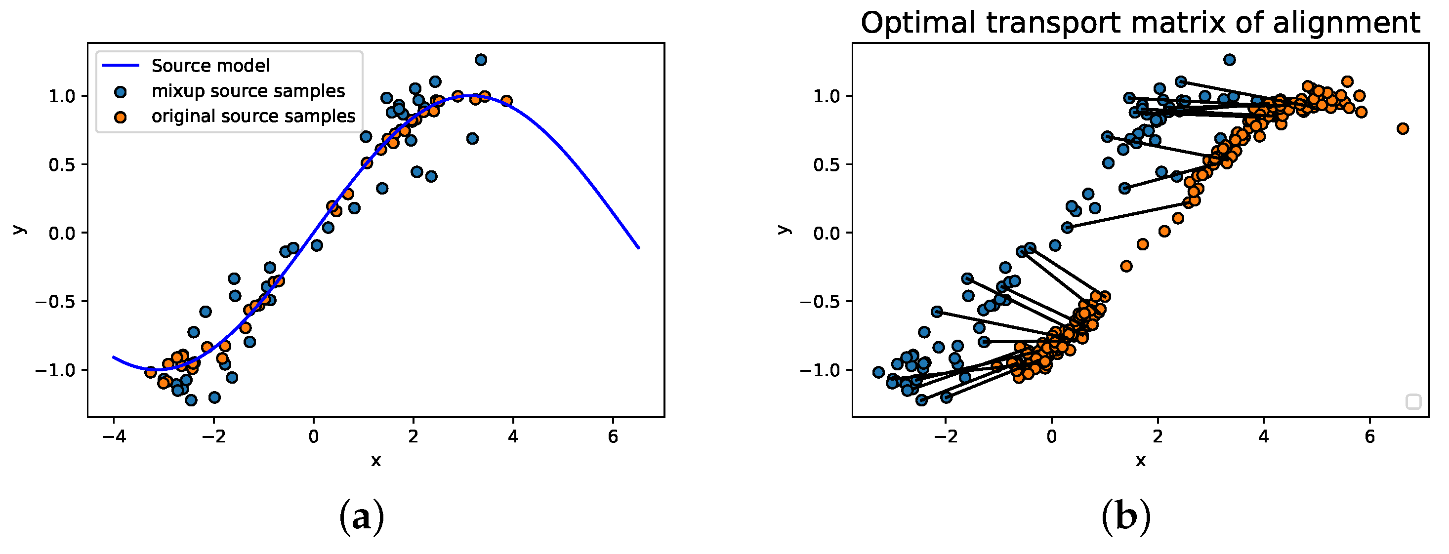
The new source samples are visualized in Figure 3a. The orange dots are the original source samples, and the blue dots are the augmented samples. The distribution of the new source domain has changed but still is a constraint in a certain bound. Then, we applied the mixup optimal transport embedded neural network on the new source domain and the target domain. The alignment results of the two distributions based on the mixup optimal transport model are shown in Figure 3b, which demonstrates the optimal matrix on the two distributions, and we can see that the augmented samples play an important role in the alignment. The mixup optimal transport-based regression model has better generalization ability.

4.2. Classification Examples

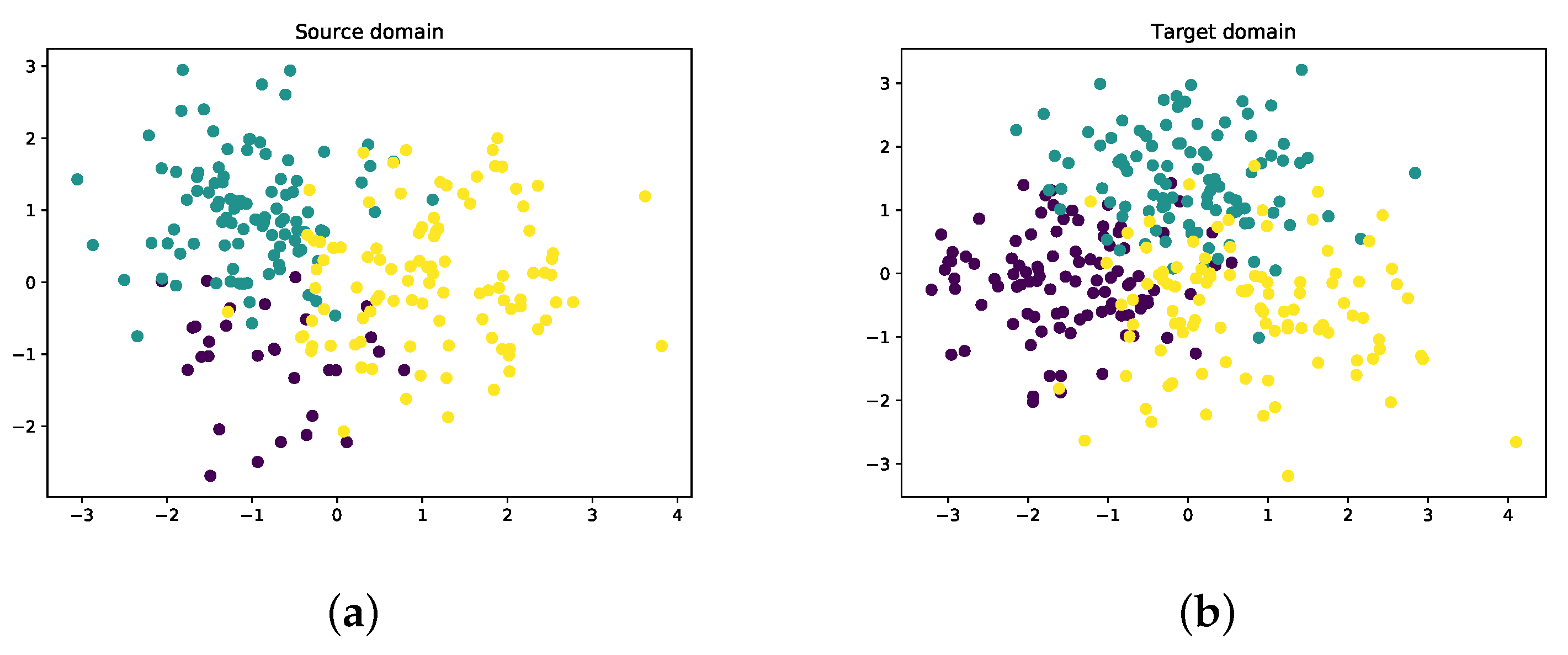
Then, we test our proposed model on fairness transfer learning classification tasks. Samples are generated following three Gaussian distributions: one of the categories only contains 30 instances, and the other two categories have 100 instances in each category. The visualization of the source domain and target domain is presented in Figure 4. Figure 4a is the distribution of the source domain, the class represented by the purple dots is the minority set, and the other two classes in yellow and green dots are the default set. Figure 4b is the distribution of the target domain. From the figures, we can see that the samples in the two domains lie in quite different distributions. If the model trained on the source domain is directly utilized in the target domain, the classification results are not competitive at all.

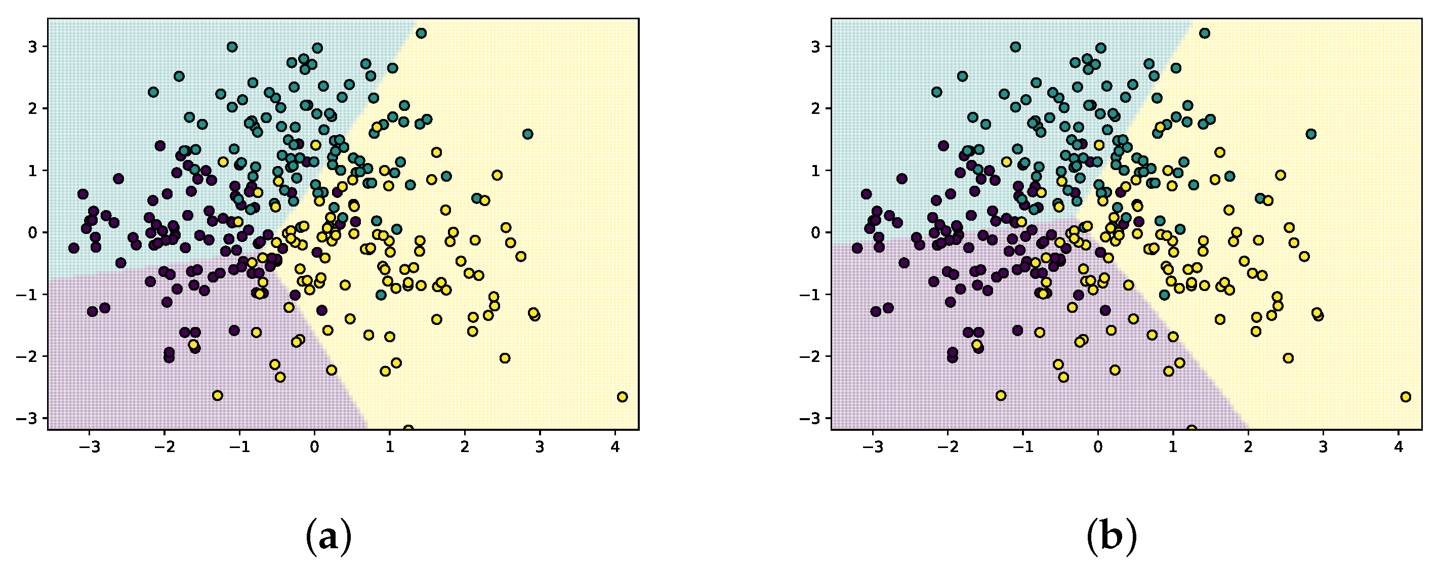
The classification results of the baseline JDOT and the proposed mixup optimal transport model are reported in Figure 5. Figure 5a is the classification result of JDOT, and Figure 5b is the result of the proposed mixup optimal transport model. The classifier trained with the mixup source domain has a larger and more correct classification area, which implies that the mixup term has a significant contribution to the fairness classification problem compared with the baseline JDOT. The purple area in Figure 5b is larger than that in Figure 5a, and the classifier bound in Figure 5b is more accurate.

4.3. Digital Classification

Then, we estimate the proposed optimal transport-embedded neural network and some domain adaptation methods in digit classification tasks on MNIST and USPS datasets. Both datasets have a 10-class classification problem and contain pictures of numbers from 0 to 9. The MNIST dataset contains 60,000 samples for training and 10,000 samples for testing. The USPS dataset has 7291 samples for training and 2007 samples for testing. The images are in grayscale.

In the transfer classification tasks, experiments are under (5-way, 10-shot) setting, which means 5 classes are selected as the minority set, and the other 5 classes are the default set. The minority set only contains 10 samples for each class, and the classes in the default set have sufficient training samples. In the experiments, only the training samples are utilized for such transfer tasks. For example, in the MNIST→USPS transfer tasks, the 60,000 training samples in the MNIST dataset are used for training, and the 7291 training samples in the USPS dataset are for testing. And we conduct the two transfer learning tasks in this subsection, MNIST→USPS, and USPS→MNIST tasks. We compared with the classifier trained on the source domain and applied it on the target domain without any alignment strategy, denoted as “CLF” in the results table, also compared with the domain adaptation methods DANN [24], MCD [25].

The comparison results are shown in

Table 1. Accuracy (%) of fairness transfer learning tasks (5-way, 10-shot) on MNIST and USPS datasets.

Method	CLF [26]	DANN [24]	MCD [25]	Ours
MNIST→USPS	40.67	42.69	41.27	55.93
USPS→MNIST	50.61	52.04	51.32	56.37

. The domain adaptation methods DANN and MCD are slightly higher than the simple classifier trained on the source domain, but the results are not ideal. And the results of the proposed mixup optimal transport model are much higher than the other domain adaptation methods. Compared with the second-highest method in Table 1, the proposed method is almost $13\%$ higher in MNIST→USPS task and about $4\%$ higher in USPS→MNIST task. The comparison results prove that the proposed mixup optimal transport model can improve the fairness transfer learning problem.

4.4. Domain Adaptation

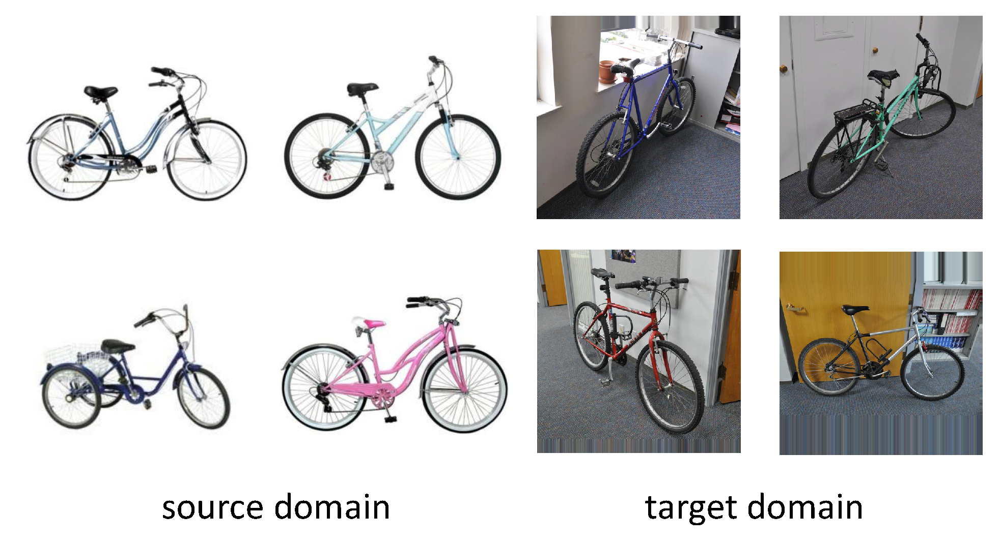
Moreover, we evaluate the model on two well-known datasets, namely Office [27] and OfficeHome [28]. The Office dataset is a real-world dataset. Amazon, DSLR, and Webcam are 3 of the 31 classes it has. A demonstration of the samples from the different domains is presented in Figure 6. In this dataset, experiments are carried out with 1-shot and 3-shot source labels per class. OfficeHome dataset has 65 classes in 4 domains (Art, Clipart, Product, and Real). According to the widely used settings [29], we examine the settings with 3% and 6% labeled source photos per class.

The foundation of the studies is the ResNet-50 pre-trained on ImageNet [30]. We employ SGD with 64 batches, a learning rate of 0.01, and a momentum of 0.9. The proposed method is compared with several state-of-the-art methods on the fairness domain adaptation problem (few-shot unsupervised domain adaptation). The classifier that trained on the source domain and tested on the target domain is denoted as CLF in the following tables. Also, the proposed method are compared with MME [31], CDAN [32], CAN [33], and CDS [29].

The experiment results of the above methods on Office and OfficeHome datasets under different few-shot settings are presented in

Table 2. Accuracy (%) of fairness transfer learning tasks 1-shot per class on Office dataset.

Method	Office
	A→D	A→W	D→A	D→W	W→A	W→D	Avg.
CLF [26]	27.5	28.7	40.9	65.2	41.1	62.0	44.2
MME [31]	21.5	12.2	23.1	60.9	14.0	62.4	32.3
CDAN [32]	11.2	6.2	9.1	54.8	10.4	41.6	22.2
CAN [33]	25.3	26.4	23.9	69.4	21.2	67.3	38.9
CDS [29]	33.3	35.2	52.0	59.0	46.5	57.4	47.2
Ours	36.6	43.5	47.1	75.0	48.2	61.4	52.0

,

Table 3. Accuracy (%) of fairness transfer learning tasks 3-shot per class on Office dataset.

Method	Office
	A→D	A→W	D→A	D→W	W→A	W→D	Avg.
CLF [26]	49.2	46.3	55.3	85.5	53.8	86.1	62.7
MME [31]	51.0	54.6	60.2	89.7	52.3	91.4	66.5
CDAN [32]	43.7	50.1	65.1	91.6	57.0	89.8	66.2
CAN [33]	48.6	45.3	41.2	78.2	39.3	82.3	55.8
CDS [29]	57.0	58.6	67.6	86.0	65.7	81.3	69.3
Ours	69.7	73.2	65.2	86.1	65.0	80.1	73.2

,

Table 4. Accuracy (%) of fairness transfer learning tasks 3% labeled source samples per class on OfficeHome dataset.

Method	OfficeHome
	Ar	Ar	Ar	Cl	Cl	Cl	Pr	Pr	Pr	Rw	Rw	Rw	Avg.
	↓	↓	↓	↓	↓	↓	↓	↓	↓	↓	↓	↓
	Cl	Pr	Rw	Ar	Pr	Rw	Ar	Cl	Rw	Ar	Cl	Pr
CLF [26]	24.4	38.3	43.1	26.4	34.7	33.7	27.5	26.5	42.6	41.2	29.0	52.3	35.0
MME [31]	4.5	15.4	25.0	28.7	34.1	37.0	25.6	25.4	44.9	39.3	29.0	52.0	30.1
CDAN [32]	5.0	8.4	11.8	20.6	26.1	27.5	26.6	27.0	40.3	38.7	25.5	44.9	25.2
CAN [33]	17.1	30.5	33.2	22.5	34.5	36.0	18.5	19.4	41.3	28.7	18.6	43.2	28.6
CDS [29]	33.5	41.1	41.9	45.9	46.0	49.3	44.7	37.8	51.0	51.6	35.7	53.8	44.4
Ours	32.2	37.2	42.2	39.3	41.5	39.4	50.7	44.9	62.9	61.3	48.4	60.6	46.8

, and

Table 5. Accuracy (%) of fairness transfer learning tasks 6% labeled source samples per class on OfficeHome dataset.

Method	OfficeHome
	Ar	Ar	Ar	Cl	Cl	Cl	Pr	Pr	Pr	Rw	Rw	Rw	Avg.
	↓	↓	↓	↓	↓	↓	↓	↓	↓	↓	↓	↓
	Cl	Pr	Rw	Ar	Pr	Rw	Ar	Cl	Rw	Ar	Cl	Pr
CLF [26]	28.7	45.7	51.2	31.9	39.8	44.1	37.6	30.8	54.6	49.9	36.0	61.8	42.7
MME [31]	27.6	43.2	49.5	41.1	46.6	49.5	43.7	30.5	61.3	54.9	37.3	66.8	46.0
CDAN [32]	26.2	33.7	44.5	34.8	42.9	44.7	42.9	36.0	59.3	54.9	40.1	63.6	43.6
CAN [33]	20.4	34.7	44.7	29.0	40.4	38.6	33.3	21.1	53.4	36.8	19.1	58.0	35.8
CDS [29]	38.8	51.7	54.8	53.2	53.3	57.0	53.4	44.2	65.2	63.7	45.3	68.6	54.1
Ours	43.1	50.6	62.3	52.9	54.2	61.0	55.5	45.6	69.9	66.7	53.7	73.7	57.4

, respectively. We can see that the proposed MixupJDOT outperforms all the other methods in all the benchmarks. Compared with the second-best method, the proposed method makes large improvements: 4.8% and 3.9% on the Office dataset, 2.4% and 3.3% on the OfficeHome dataset. The results demonstrate the efficiency of the proposed method in fairness transfer learning scenarios.

5. Conclusions

In this paper, a novel mixup optimal transport embedded neural network is constructed based on the joint distribution optimal transport theory. The proposed neural network targets the fairness transfer learning problem, and the mixup mechanism is adapted to augment the training source samples on convex combinations of pairs of examples and their labels. Experiments on regression and classification results verified that the proposed methods could significantly improve performance under fairness settings. In fairness transfer learning tasks using 3% labeled source samples per class on the OfficeHome dataset, which is the most challenging benchmark, the experimental findings demonstrate that our method’s accuracy is 2.4% greater than that of the second-best mode. On the OfficeHome dataset, where transfer learning tasks 6% identified source samples per class, our method’s accuracy is 3.3% higher than the second-best mode. However, there are still some drawbacks to the proposed method. Only data regression and image classification are employed in this paper’s application, and there is only one data modality. In future work, we will try to extend the framework to a more complicated model for several widely used benchmarks and real-world applications and utilize the model to power edge AI applications.