Analysis of Function Approximation and Stability of General DNNs in Directed Acyclic Graphs Using Un-Rectifying Analysis

Abstract

A general lack of understanding pertaining to deep feedforward neural networks (DNNs) can be attributed partly to a lack of tools with which to analyze the composition of non-linear functions, and partly to a lack of mathematical models applicable to the diversity of DNN architectures. In this study, we analyze DNNs using directed acyclic graphs (DAGs) under a number of basic assumptions pertaining to activation functions, non-linear transformations, and DNN architectures. DNNs that satisfy these assumptions are referred to as general DNNs. Our construction of an analytic graph was based on an axiomatic method in which DAGs are built from the bottom–up through the application of atomic operations to basic elements in accordance with regulatory rules. This approach allowed us to derive the properties of general DNNs via mathematical induction. We demonstrate that the proposed analysis method enables the derivation of some properties that hold true for all general DNNs, namely that DNNs “divide up” the input space, “conquer” each partition using a simple approximating function, and “sparsify” the weight coefficients to enhance robustness against input perturbations. This analysis provides a systematic approach with which to gain theoretical insights into a wide range of complex DNN architectures.

1. Introduction

Deep feedforward neural networks (DNNs) have revolutionized the use of machine learning in many fields, such as computer vision and signal processing, where they have been used to resolve ill-posed inverse problems and sparse recovery problems [1,2]. Much of the previous research in the field of deep learning literature describes the construction of neural networks capable of attaining a desired level of performance for a given task. However, researchers have yet to elucidate several fundamental issues that are critical to the function of DNNs. Predictions that are based on a non-explainable and non-interpretable models raise trust issues pertaining to the deployment of that neural network in practical applications [3]. This lack of understanding can be attributed, at least partially, to a lack of tools with which to analyze the composition of non-linear activation functions in DNNs, as well as a lack of mathematical models applicable to the diversity of DNN architectures. This paper reports on a preliminary study of fundamental issues pertaining to function approximation and the inherent stability inherent of DNNs.

Simple series-connected DNN models, such as ${\mathcal{N}}_L^s\left(\mathbf{x}\right)={\varrho }_L\circ M_L\circ \cdots \circ {\varrho }_1\circ M_1\left(\mathbf{x}\right)$, have been widely adopted for analysis [4,5,6]. According to this model, the input domain is partitioned into a collection of polytopes in a tree-like manner. Each node of the tree can be associated with a polytope and one affine linear mapping, which gives a local approximation of an unknown target function with a domain restriction on the polytope [7,8]. We initially considered whether the theoretical results derived in those papers were intrinsic/common to all DNNs or unique to this type of network. However, our exploration of this issue was hindered by problems encountered in representing a large class of DNN architectures and in formulating the computation spaces for activation functions and non-linear transformations. In our current work, we addressed the latter problem by assuming that all activation functions can be expressed as networks with point-wise continuous piecewise linear (CPWL) activation functions and that all non-linear transforms are Lipschitz functions. The difficulties involved in covering all possible DNNs prompted us to address the former problem by associating DNNs with graphs that can be described in a bottom–up manner using an axiomatic approach, thereby allowing for analysis of each step in the construction process. This approach made it possible for us to build complex networks from simple ones and derive their intrinsic properties via mathematical induction.

In the current study, we sought to avoid the generation of graphs with loops by describing DNNs using directed acyclic graphs (DAGs). The arcs are associated with basic elements that correspond to operations applied to the layers of a DNN (e.g., linear matrix, affine linear matrix, non-linear activation function/transformation), while nodes that delineate basic elements are used to relay and reshape the dimension of an input or combine outputs from incoming arcs to outgoing arcs. We refer to DNNs that can be constructed using the proposed axiomatic approach as general DNNs. It is unclear whether general DNNs are equivalent to all DNNs that are expressible using DAGs. Nevertheless, general DNNs include modules widely employed in well-known DNN architectures. The proposed approach makes it possible to extend the theoretical results for series-connected DNNs to general DNNs, as follows:

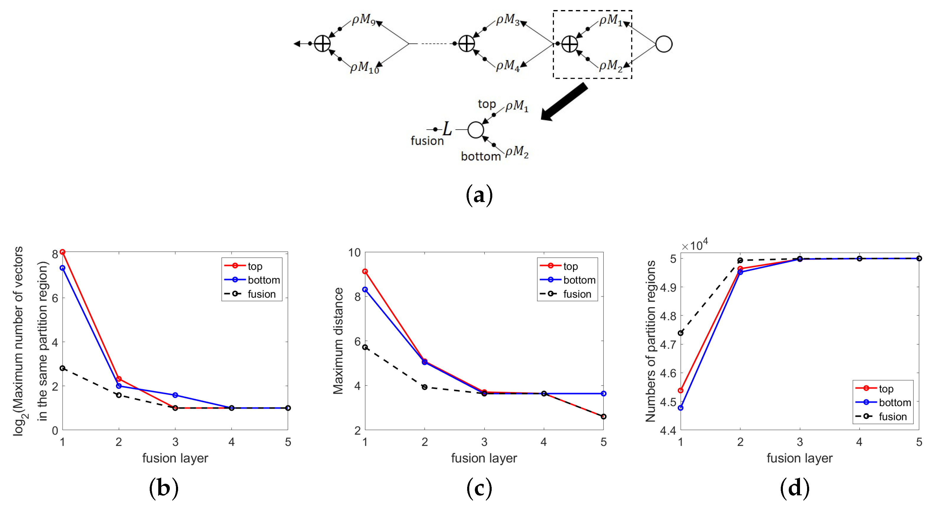
• A DNN DAG divides the input space via partition refinement using either a composition of activation functions along a path or a fusion operation combining inputs from more than one path in the graph. This makes it possible to approximate a target function in a coarse-to-fine manner by applying a local approximating function to each partitioning region in the input space. Furthermore, the fusion operation means that domain partition tends not to be a tree-like process.
• Under mild assumptions related to point-wise CPWL activation functions and non-linear transformations, the stability of a DNN against local input perturbations can be maintained using sparse/compressible weight coefficients associated with incident arcs to a node.

Accordingly, we can conclude that a general DNN “divides” the input space, “conquers” the target function by applying a simple approximating function over each partition region, and “sparsifies” weight coefficients to enhance robustness against input perturbations.

In the literature, graphs are commonly used to elucidate the structure of DNNs; however, they are seldom used to further the analysis of DNNs. Both graph DNNs [9] and the proposed approach adopt graphs for analysis; however, graph DNNs focus on the operations of neural networks in order to represent real-world datasets in graphs (e.g., social networks and molecular structure [10]), whereas our approach focuses on the construction of analyzable graph representations by which to deduce intrinsic properties of DNNs.

The remainder of this paper is organized as follows. In Section 2, we present a review of related works. Section 3 outlines our bottom–up axiomatic approach to the construction of DNNs. Section 4 outlines the function approximation and stability of general DNNs. Concluding remarks are presented in Section 5.

Notation 1.

Matrices are denoted using bold upper case, and vectors are denoted using bold lower case. We also use $x_i$ to denote the i-th entry of a vector ($\mathbf{x}\in {\mathbb{R}}^n$), ${\parallel \mathbf{x}\parallel }_2$ to denote its Euclidean norm, and $diag\left(\mathbf{x}\right)$ to denote a diagonal matrix with diagonal $\mathbf{x}$.

2. Related Works

Below, we review analytic methods that are applicable to the derivation of network properties with the aim of gaining a more complete understanding of DNNs.

The ordinary differential equation (ODE) approach was originally inspired by a residual network (ResNet) [11], which is regarded as a discrete implementation of an ODE [12]. The ODE approach can be used to interpret networks by treating them as different discretizations of different ODEs. Note that the process of developing numerical methods for ODEs makes it possible to develop new network architectures [13]. The tight connection between the ODE and dynamic systems [14] makes it possible to study the stability of forward inference in a DNN and the well-posedness of learning a DNN (i.e., whether a DNN can be generalized by adding appropriate regularizations or training data), in which the stability of the DNN is related to initial conditions, while network design is related to the design of a system of the ODE system. The ODE approach can also be used to study recurrent networks [15]. Nevertheless, when adopting this approach, one must bear in mind that the conclusions of an ODE cannot be applied to the corresponding DNN in a straightforward manner due to the fact that a numerical ODE may undergo several discretization approximations (e.g., forward/backward Euler approximations), which can generate inconsistent results [16].

Some researchers have sought to use existing knowledge of signal processing in the design of DNN-like networks that are more comprehensive without sacrificing performance. This can often be achieved by replacing non-linear activation functions with interpretable non-linear operations in the form of non-linear transforms. Representative examples include the scattering transform [17,18] and Saak transform [19]. Scattering transform takes advantage of the wavelet transform and scattering operations in physics. Saak transform employs statistical methods with invertible approximations.

Network design was also inspired by the methods used in optimization algorithms to solve ill-posed inverse problems [20]. The unrolling approach involves the systematic transformation of an iterative algorithm (for an ill-posed inverse problem) into a DNN. The number of iterations becomes the number of layers, and the matrix in any given iteration is relaxed through the use of affine linear operations and activation functions. This makes it possible to infer the solution of the inverse problem by using a DNN. This is an efficient approach to deriving a network for an inverse problem and often achieves performance exceeding the theoretical guarantees for conventional methods [21,22]; however, it does not provide sufficient insight into the properties of DNNs that are capable of solving the inverse problem. A thorough review of this topic can be found in [2].

The un-rectifying method is closely tied to the problem-solving method used in piecewise functions, wherein the domain is partitioned into intervals to be analyzed separately. This approach takes advantage of the fact that a piecewise function is generally difficult to analyze as a whole but is a tractable function when the domain is restricted to a partitioned interval. When applying the un-rectifying method, a point-wise CPWL activation function is replaced with a finite number of data-dependent linear mappings. This makes it possible to associate different inputs with different functions. The method replaces the point-wise CPWL activation function as a data-dependent linear mapping, as follows:

$$\begin{array}{c}\hfill \rho \left(\mathbf{x}\right)={\mathbf{D}}_{\mathbf{x}}^{\rho }\left(\mathbf{x}\right),\end{array}$$

(1)

where ${\mathbf{D}}_{\mathbf{x}}^{\rho }$ is the un-rectifying matrix for $\rho$ at $\mathbf{x}$. If $\rho$ is the ReLU, then ${\mathbf{D}}_{\mathbf{x}}^{\rho }$ is a diagonal matrix with diagonal entries $\{0,1\}$. The un-rectifying variables in the matrix provide crucial clues according to which to characterize the function of the DNN. For example, comparing the following un-rectifying representation of $M_2\circ {\mathcal{N}}_1^s$ with inputs $\mathbf{x}$ and $\mathbf{y}$ yields

$$\begin{array}{cc}\hfill M_2\circ {\mathcal{N}}_1^s\left(\mathbf{x}\right)& =M_2{\mathbf{D}}_{M_1\mathbf{x}}{M}_1\left(\mathbf{x}\right)\hfill \end{array}$$

(2)

$$\begin{array}{cc}\hfill M_2\circ {\mathcal{N}}_1^s\left(\mathbf{y}\right)& =M_2{\mathbf{D}}_{M_1\mathbf{y}}{M}_1\left(\mathbf{y}\right).\hfill \end{array}$$

(3)

Note that the sole difference between (2) and (3) lies in the un-rectifying matrices (${\mathbf{D}}_{M_1\mathbf{x}}$ and ${\mathbf{D}}_{M_1\mathbf{y}}$, respectively). This is illustrated in the following example involving the application of the un-rectifying method to the analysis of domain partitioning in a neural network. Refer to [5] for more examples of the approach.

Un-Rectifying Analysis

Consider a simple regression model comprising a sequence of composition operations:

$$\begin{array}{c}\hfill {\mathcal{R}}_L=M_L\left({\mathrm{ReLU}}_{L-1}\right)M_{L-1}\cdots \left({\mathrm{ReLU}}_1\right)M_1=M_L{\mathcal{N}}_{L-1}\end{array}$$

(4)

where $\left\{M_i\right\}$ denotes affine linear mappings and ${\mathrm{ReLU}}_k:{\mathbb{R}}^{l_k}\to {\mathbb{R}}^{l_k}$. Theoretical results for this network were derived using affine spline insights [4] and the un-rectifying method [5,23].

When considering an input space partitioned using (4), it is important to consider the ReLU activation functions due to the fact that affine linear mappings are global continuous functions. Let ${\mathbb{P}}_k$ denote the finest input domain partition generated by ${\mathcal{N}}_k$. Appending an additional layer ($\left({\mathrm{ReLU}}_{k+1}\right)M_{k+1}$) to ${\mathcal{N}}_k$ refines partition ${\mathbb{P}}_k$, which results in ${\mathbb{P}}_{k+1}\subseteq {\mathbb{P}}_k$ (i.e., every partitioning region in ${\mathbb{P}}_{k+1}$ is contained in one of the partitioning regions in ${\mathbb{P}}_k$) [5]. Below, we demonstrate that partitioning regions can be expressed via induction using an un-rectifying representation of ReLUs.

Consider the basic case of a single ReLU layer:

$$\begin{array}{c}\hfill \left({\mathrm{ReLU}}_1\right)M_1\mathbf{x}={\mathbf{D}}_1{M}_1\mathbf{x}={\mathbf{s}}_1\odot M_1\mathbf{x},\end{array}$$

(5)

where state vector ${\mathbf{s}}_1\in {\{0,1\}}^{l_1}$ lists diagonal entries in ${\mathbf{D}}_1$, the values of which depend on $M_1\mathbf{x}$. Input space $\chi$ is partitioned by hyperplanes derived from the rows of $M_1$ into no more than $2^{l_1}$ partitioning regions. Let ${\mathbf{S}}_1$ denote the collection of all possible ${\mathbf{s}}_1$ vectors, and let $|{\mathbf{S}}_1|$ denote its size. The fact that each partitioning region in ${\mathbb{P}}_1$ can be associated with precisely one element in ${\mathbf{S}}_1$ means that partitioning regions can be treated as indices using vector ${\mathbf{s}}_1$. The partitioning region indexed by vector ${\mathbf{s}}_1$ as $R_{{\mathbf{s}}_1}$ for $\mathbf{x}\in R_{{\mathbf{s}}_1}$ can be characterized as an intersection of half-spaces:

$$\begin{array}{c}\hfill \left\{\begin{array}{c}{\left(M_1\mathbf{x}\right)}_i>0\mathrm{if}{\left({\mathbf{s}}_1\right)}_i=1(\mathrm{the}i-\mathrm{th}\mathrm{element}\mathrm{of}\mathrm{vector}{\mathbf{s}}_1)\hfill \\ {\left(M_1\mathbf{x}\right)}_i\le 0\mathrm{if}{\left({\mathbf{s}}_1\right)}_i=0.\hfill \end{array}\right.\end{array}$$

(6)

Thus, regression function ${\mathcal{R}}_2$ comprises $|{\mathbf{S}}_1|$ partitioning regions. When restricted to region ${\mathcal{R}}_{{\mathbf{s}}_1}$, the function is $M_2{\mathbf{s}}_1\odot M_1$. Figure 1 illustrates the input domain partitioning of ${\mathcal{R}}_1={\mathcal{M}}_1=\left({\mathrm{ReLU}}_1\right)M_1$, where

$$M_1(\left[\begin{array}{c}x\\ y\end{array}\right])=\left[\begin{array}{c}0\\ 0\end{array}\right]+\left[\begin{array}{cc}1& 1\\ -1& 1\end{array}\right]\left[\begin{array}{c}x\\ y\end{array}\right].$$

(7)

${\mathcal{R}}_1$ consists of two hyperplanes ($h_1=x+y=0$ and $h_2=y-x=0$), which divide ${\mathbb{R}}^2$ into partition ${\mathbb{P}}_1$ comprising regions I, $II$, $III$, and $IV$. Region I is characterized by $h_1\left(\mathbf{x}\right)>0$ and $h_2\left(\mathbf{x}\right)>0$, while region $II$ is characterized by $h_1\left(\mathbf{x}\right)\le 0$ and $h_2\left(\mathbf{x}\right)>0$, etc.

Now, consider two layers of ReLUs: ${\mathcal{N}}_2=\left({\mathrm{ReLU}}_2\right)M_2\left({\mathrm{ReLU}}_1\right)M_1={\mathbf{D}}_2{M}_2{\mathbf{D}}_1{M}_1$, where the finest partition of ${\mathcal{N}}_2$ as ${\mathbb{P}}_2$; $|{\mathbf{S}}_2|$ indicates the size of ${\mathbf{S}}_2$, and ${\mathbf{S}}_2$ refers to a collection of all possibles vectors ($\mathbf{s}={\left[{\mathbf{s}}_2^{\top }{\mathbf{s}}_1^{\top }\right]}^{\top }$, where ${\mathbf{s}}_2\in {\{0,1\}}^{l_2}$). Each partitioning region of ${\mathbb{P}}_2$ can be associated with precisely one element in ${\mathbf{S}}_2$ and one affine linear mapping. Given that $\mathbf{s}\in {\mathbf{S}}_2$, the partitioning region indexed by $\mathbf{s}$ is denoted as $R_{\mathbf{s}}$, where any $\mathbf{x}\in R_{\mathbf{s}}$ can be characterized as an intersection of half-space as follows:

$$\begin{array}{c}\hfill \left\{\begin{array}{c}{\left(M_2{\mathbf{D}}_1{M}_1\mathbf{x}\right)}_i={(M_2{\mathbf{s}}_1\odot M_1\mathbf{x})}_i>0\mathrm{if}{\left({\mathbf{s}}_2\right)}_i=1\hfill \\ {\left(M_2{\mathbf{D}}_1{M}_1\mathbf{x}\right)}_i={(M_2{\mathbf{s}}_1\odot M_1\mathbf{x})}_i\le 0\mathrm{if}{\left({\mathbf{s}}_2\right)}_i=0\hfill \\ {\left(M_1\mathbf{x}\right)}_j>0\mathrm{if}{\left({\mathbf{s}}_1\right)}_j=1\hfill \\ {\left(M_1\mathbf{x}\right)}_j\le 0\mathrm{if}{\left({\mathbf{s}}_1\right)}_j=0.\hfill \end{array}\right.\end{array}$$

(8)

The last two inequalities in (8) are equivalent to $\mathbf{x}\in R_{{\mathbf{s}}_1}$, such that

$$\begin{array}{c}\hfill R_{\mathbf{s}}=\left\{\begin{array}{c}{\left(M_2{\mathbf{D}}_1{M}_1\mathbf{x}\right)}_i={(M_2{\mathbf{s}}_1\odot M_1\mathbf{x})}_i>0\mathrm{if}{\left({\mathbf{s}}_2\right)}_i=1\hfill \\ {\left(M_2{\mathbf{D}}_1{M}_1\mathbf{x}\right)}_i={(M_2{\mathbf{s}}_1\odot M_1\mathbf{x})}_i\le 0\mathrm{if}{\left({\mathbf{s}}_2\right)}_i=0\hfill \\ \mathbf{x}\in R_{{\mathbf{s}}_1}.\hfill \end{array}\right.\end{array}$$

(9)

The first two inequalities in (9) divide $R_{{\mathbf{s}}_1}$ according to the value of ${\mathbf{s}}_2$. This means that $R_{\mathbf{s}}\subseteq R_{{\mathbf{s}}_1}$, which allows us to express ${\mathbf{S}}_2=\left\{{\left[{\mathbf{s}}_1^{\top }{\mathbf{s}}_2^{\top }\right]}^{\top }\right|{\mathbf{s}}_1\in {\mathbf{S}}_1\}$, where vector ${\mathbf{s}}_2$ is dependent/conditional on ${\mathbf{s}}_1$. Regression function ${\mathcal{R}}_3$ comprises $|{\mathbf{S}}_2|$ partitioning regions. When restricted to $R_{\mathbf{s}}$ with $\mathbf{s}={\left[{\mathbf{s}}_1^{\top }{\mathbf{s}}_2^{\top }\right]}^{\top }\in {\mathbf{S}}_2$, the function is $M_3{\mathbf{s}}_2\odot M_2{\mathbf{s}}_1\odot M_1$.

Example 1.

Given ${\mathcal{R}}_2={\mathcal{M}}_2=\left({\mathit{ReLU}}_2\right)M_2\left({\mathit{ReLU}}_1\right)M_1$, where $M_1$ is given in (7) and

$$M_2(\left[\begin{array}{c}x\\ y\end{array}\right])=\left[\begin{array}{c}-4\\ -3\end{array}\right]+\left[\begin{array}{cc}1& 0.3\\ -0.3& 1\end{array}\right]\left[\begin{array}{c}x\\ y\end{array}\right].$$

(10)

Let ${\mathbf{s}}_1={\left[s_1{s}_2\right]}^{\top }$ be the list of diagonal entries in ${\mathbf{D}}_1$. Then,

$$\begin{array}{c}\hfill M_2\left({\mathit{ReLU}}_1\right)M_1(\left[\begin{array}{c}x\\ y\end{array}\right])=\left[\begin{array}{c}-4\\ -3\end{array}\right]+\left[\begin{array}{cc}1& 0.3\\ -0.3& 1\end{array}\right]\left[\begin{array}{c}{s}_1(x+y)\\ s_2(y-x)\end{array}\right].\end{array}$$

(11)

In region I, where ${\mathbf{s}}_1={\left[11\right]}^{\top }$, we obtain

$$\begin{array}{c}\hfill {\mathcal{R}}_2(\left[\begin{array}{c}x\\ y\end{array}\right])=\left({\mathit{ReLU}}_2\right)\left[\begin{array}{c}-4+0.7x+1.3y\\ -3-1.3x+0.7y\end{array}\right]\end{array}$$

(12)

In region $II$, where ${\mathbf{s}}_1={\left[01\right]}^{\top }$, we obtain

$$\begin{array}{c}\hfill {\mathcal{R}}_2(\left[\begin{array}{c}x\\ y\end{array}\right])=\left({\mathit{ReLU}}_2\right)\left[\begin{array}{c}-4+0.3(y-x)\\ -3+y-x\end{array}\right],\end{array}$$

(13)

the components of which are parallel to $h_2=y-x=0$.

In region $IV$, where ${\mathbf{s}}_1={\left[10\right]}^{\top }$, we obtain

$$\begin{array}{c}\hfill {\mathcal{R}}_2(\left[\begin{array}{c}x\\ y\end{array}\right])=\left({\mathit{ReLU}}_2\right)\left[\begin{array}{c}-4+y+x\\ -3-0.3(y+x)\end{array}\right],\end{array}$$

(14)

the components of which are parallel to $h_1=y+x=0$.

In region $III$, where ${\mathbf{s}}_1={\left[00\right]}^{\top }$,

$$\begin{array}{c}\hfill {\mathcal{R}}_2(\left[\begin{array}{c}x\\ y\end{array}\right])=\left({\mathit{ReLU}}_2\right)\left[\begin{array}{c}-4\\ -3\end{array}\right]=.\end{array}$$

(15)

All points in this region are mapped to the zero vector. Figure 2 shows input domain partition $P_2$ of ${\mathcal{R}}_2$.

3. DNNs and DAG Representations

The class of DNNs addressed in this study is defined by specific activation functions, non-linear transformations, and its underlying architecture. Note that legitimate activation functions, non-linear transformations, and architectures should be analyzable and provide sufficient generalizability to cover all DNNs in common use.

Activation functions and non-linear transformations are both considered functions; however, we differentiate between them due to differences in the way they are treated under un-rectifying analysis. A non-linear transformation is a function in the conventional sense when mapping ${\mathbb{R}}^n$ to ${\mathbb{R}}^m$, in which different inputs are evaluated using the same function. This differs from activation functions, in which different inputs can be associated with different functions. For example, for ReLU $\mathbb{R}\to \mathbb{R}$, un-rectifying considers $\mathrm{ReLU}x=dx$ where $d\in \{0,1\}$ as two functions depending on whether $x>0$ where $d=1$ or $x\le 0$ where $d=0$.

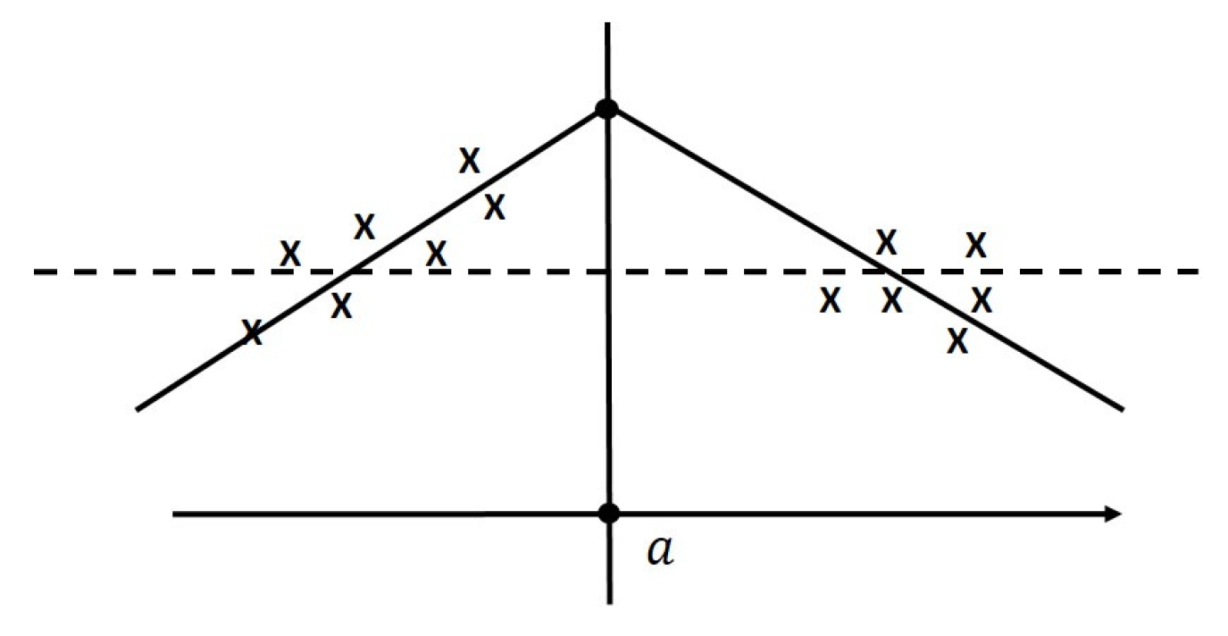
3.1. Activation Functions and Non-Linear Transformations

In this paper, we focus on activation functions that can be expressed as networks of point-wise CPWL activation functions ($\rho$). Based on this assumption and the following lemma, we assert that the activation functions of concern are ReLU networks.

Lemma 1

([24]). Any point-wise CPWL activation function ($\rho :\mathbb{R}\to \mathbb{R}$) of m pieces can be expressed as follows:

$$\begin{array}{cc}\hfill \rho \left(x\right)& =\sum _{i=1}^m{r}_i\mathit{ReLU}(x-a_i)+l_i\mathit{ReLU}(t_i-x)\hfill \\ \hfill & =\sum _{i\in I^{+}}{r}_i\mathit{ReLU}(x-a_i)+\sum _{i\in I^{-}}{l}_i\mathit{ReLU}(t_i-x)\hfill \end{array}$$

(16)

where $l_i$ and $r_i$ indicate the slopes of segments and $a_i$ and $t_i$ are breakpoints of the corresponding segments.

Note that the max-pooling operation (arguably the most popular non-linear pooling operation), which outputs the largest value in the block and maintains the selected location [25], is also a ReLU network. The max pooling of a block of any size can be recursively derived by max pooling a block of size 2. For example, let ${max}_4$ and ${max}_2$ denote the max pooling of blocks of sizes 4 and 2, respectively. Then, ${max}_4(x_1,x_2,x_3,x_4)={max}_2({max}_2(x_1,x_2),{max}_2(x_3,x_4))$ and ${max}_5(x_1,x_2,x_3,x_4,x_5)={max}_2({max}_4(x_1,x_2,x_3,x_4),$$x_5)$. The max pooling of a block of size 2 can be expressed as follows:

$$\begin{array}{cc}\hfill {max}_2(\mathbf{x}={\left[x_1{x}_2\right]}^{\top })& =\frac{x_1+x_2}{2}+\frac{|x_1-x_2|}{2}\hfill \\ \hfill & =\frac{1}{2}\left[111\right]\tilde{\rho }\left[\begin{array}{cc}1& 1\\ 1& -1\\ -1& 1\end{array}\right]\mathbf{x},\hfill \end{array}$$

(17)

where $\tilde{\rho }\in {\mathbb{R}}^{3\times 3}$ is

$$\begin{array}{c}\hfill \tilde{\rho }=\left[\begin{array}{ccc}1& 0& 0\\ 0& \mathrm{ReLU}& 0\\ 0& 0& \mathrm{ReLU}\end{array}\right].\end{array}$$

In this paper, we make two assumptions pertaining to activation function $\rho$:

(A1)

$\rho :\mathbb{R}\to \mathbb{R}$ can be expressed as (16).

This assumption guarantees that for any input ($\mathbf{x}$), the layer of $\rho :{\mathbb{R}}^l\to {\mathbb{R}}^l$ can be associated with diagonal un-rectifying matrix ${\mathbf{D}}_{\mathbf{x}}^{\rho }$ with real-valued diagonal entries, where the value of the l-th diagonal entry is ${\sum }_{i\in I_l^{+}}{r}_{l,i}+{\sum }_{j\in I_l^{-}}{l}_{l,j}$, while $I_l^{+}$ and $I_l^{-}$ denote the sets in which ReLUs are active.

(A2)

There exists a bound that $d_{\rho }>0$ for any activation function ($\rho$) regardless of input ($\mathbf{x}$). This corresponds to the assumption that

$$\begin{array}{c}\hfill \parallel {\mathbf{D}}_{\mathbf{x}}^{\rho }{\parallel }_2\le \underset{l}{max}\sum _{i\in I_l^{+}}|r_{l,i}|+\sum _{j\in I_l^{-}}\left|l_{l,j}\right|\le d_{\rho }\end{array}$$

(18)

This assumption is used to establish the stability of a network against input perturbations.

The outputs of a non-linear transformation layer can be interpreted as coefficient vectors related to that domain of the transformation. We make the following assumption pertaining to non-linear transformation ($\sigma$) addressed in the current paper.

(A3)

There exists a uniform Lipschitz constant bound ($d_{\sigma }>0$) with respect to ${\ell }_2$ norm for any non-linear transformation function ($\sigma$) and any inputs ($\mathbf{x}$ and $\mathbf{y}$) in ${\mathbb{R}}^n$:

$$\begin{array}{c}\hfill {\parallel \sigma \left(\mathbf{x}\right)-\sigma \left(\mathbf{y}\right)\parallel }_2\le d_{\sigma }{\parallel \mathbf{x}-\mathbf{y}\parallel }_2.\end{array}$$

(19)

This assumption is used to establish the stability of a network against input perturbations. Sigmoid and tanh functions are 1-Lipschitz [26]. The softmax layer from ${\mathbb{R}}^n$ to ${\mathbb{R}}^n$ is defined as $x_i\to \frac{{exp}^{\lambda x_i}}{{\sum }_{j=1}^n{exp}^{\lambda x_j}}$, where $\lambda$ is the inverse temperature constant. The output is the estimated probability distribution of the input vector in the simplex of ${\mathbb{R}}^n$ and $i=1,\cdots ,n$. Softmax function ${\mathrm{Softmax}}_{\lambda }$ persists as $\lambda$-Lipschitz [27], as follows:

$$\begin{array}{c}\hfill \parallel {\mathrm{Softmax}}_{\lambda }\left(\mathbf{x}\right)-{\mathrm{Softmax}}_{\lambda }{\left(\mathbf{y}\right)\parallel }_2\le \lambda {\parallel \mathbf{x}-\mathbf{y}\parallel }_2.\end{array}$$

3.2. Proposed Axiomatic Method

Let $\mathcal{K}$ denote the class of DNNs that can be constructed using the following axiomatic method with activation functions that satisfy (A1) and (A2) and non-linear transformations that satisfy (A3). This axiomatic method employs three atomic operations (O1–O3), the basic set $\mathcal{B}\subseteq \mathcal{K}$, and a regulatory rule (R) describing a legitimate method by which to apply an atomic operation to elements in $\mathcal{K}$ in order to yield another element in $\mathcal{K}$.

Basis set $\mathcal{B}$ comprises the following operations:

$$\begin{array}{c}\hfill \mathcal{B}=\{\mathbf{I},\mathbf{L},M,{\Gamma }_{\rho },\rho M,{\Gamma }_{\sigma },\sigma M\},\end{array}$$

(20)

where $\mathbf{I}$ denotes the identify operation; $\mathbf{L}$ denotes any finite dimensional linear mapping with bounded spectral norms; $M=(\mathbf{L},\mathbf{b})$ denotes any affine linear mapping, where $\mathbf{L}$ and $\mathbf{b}$ refer to the linear and bias terms, respectively; ${\Gamma }_{\rho }$ denotes activation functions satisfying (A1) and (A2); $\rho M$ denotes functions with $\rho \in {\Gamma }_{\rho }$; ${\Gamma }_{\sigma }$ denotes non-linear transformations satisfying (A3); and $\sigma M$ denotes functions with $\sigma \in {\Gamma }_{\sigma }$.

Assumptions pertaining to ${\Gamma }_{\rho }$ and ${\Gamma }_{\sigma }$ are combined to obtain the following:

(A) The assumption of uniform bounding is based on the existence of a uniform bound, where $\infty >d>0$ for any activation function ($\rho \in {\Gamma }_{\rho }$), any input ($\mathbf{x}$), and any non-linear transformation ($\sigma \in {\Gamma }_{\sigma }$), such that

$$\begin{array}{c}\hfill d\ge max\{d_{\rho },d_{\sigma }\}.\end{array}$$

(21)

Let $\chi$ denote the input space for any elements in $\mathcal{B}$. The results of the following atomic operations belong to $\mathcal{K}$. The corresponding DAG representations are depicted in Figure 3 (a reshaping of input or output vectors is implicitly applied at nodes to validate these operations).

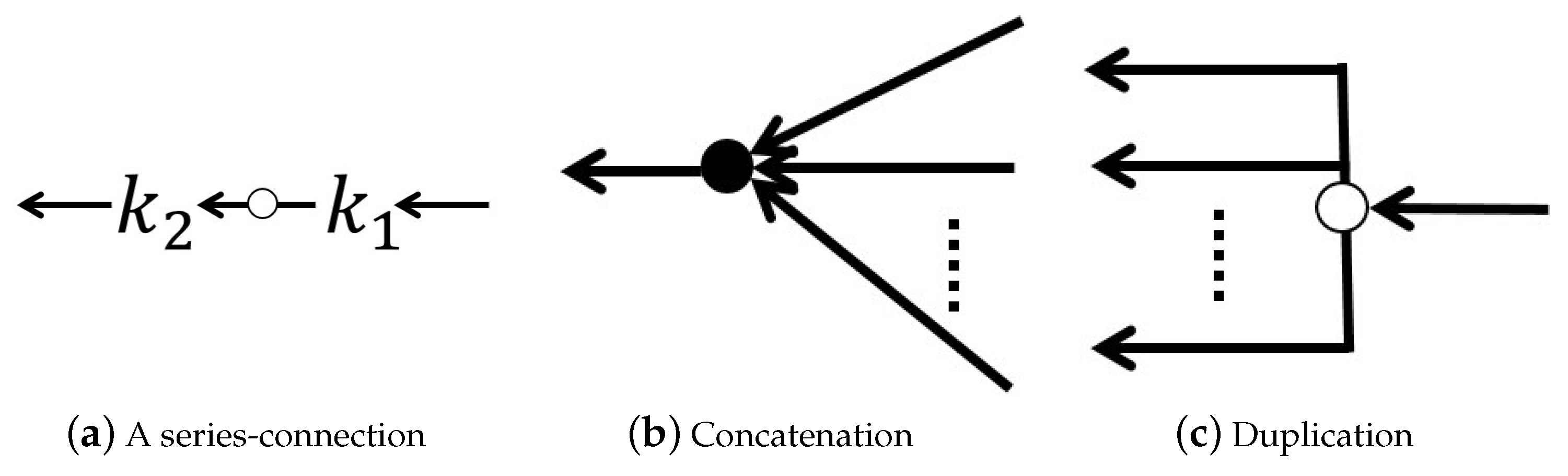
O1.

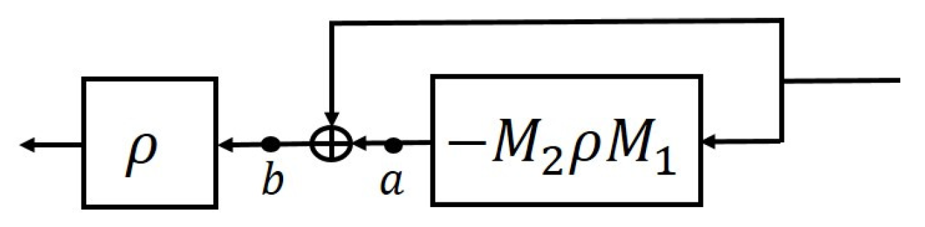
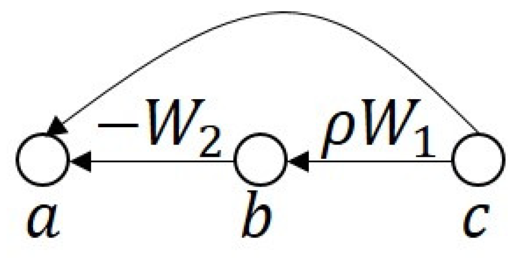
Series connection (∘): We combine $\mathcal{B}$ and $\mathcal{K}$ by letting the output of $k_1\in \mathcal{K}$ be the input of $k_2\in \mathcal{B}$, where

$$\begin{array}{c}\hfill \mathcal{B}\circ \mathcal{K}:k_2\circ k_1:\mathbf{x}\to k_2\left(k_1\mathbf{x}\right).\end{array}$$

O2.

Concatenation: We combine multichannel inputs ${\mathbf{x}}_i\in \chi$ into a vector as follows:

$$\begin{array}{c}\hfill \mathrm{concatenation}:\{{\mathbf{x}}_1,\cdots ,{\mathbf{x}}_m\}\to {[{\mathbf{x}}_1^{\top }\cdots {\mathbf{x}}_m^{\top }]}^{\top }.\end{array}$$

O3.

Duplication: We duplicate an input to generate m copies of itself as follows:

$$\begin{array}{c}\hfill \mathrm{duplication}:\mathbf{x}\in \chi \to \left[\begin{array}{c}\mathbf{I}\\ ⋮\\ \mathbf{I}\end{array}\right]\mathbf{x}.\end{array}$$

From the basic set and O1–O3, regulatory rule R generates other elements in $\mathcal{K}$ by regulating the application of atomic operations on $\mathcal{K}$. The aim of R is to obtain DNNs that can be represented as DAGs; therefore, this rule precludes the generation of graphs that contain loops.

R.

DAG closure: We apply O1–O3 to $\mathcal{K}$ in accordance with

$$\begin{array}{c}\hfill R:\mathcal{K}\to \mathcal{K}.\end{array}$$

The DAGs of $\mathcal{K}$ comprise nodes and arcs, each of which belongs to one of operations O1–O3. Rule R mandates that any member in $\mathcal{K}$ can be represented as a DAG, in which arcs are associated with members in $\mathcal{B}$ and nodes coordinate the inlets and outlets of arcs. The rule pertaining to the retention of DAGs after operations on DAGs is crucial to our analysis based on the fact that nodes in a DAG can then be ordered (see Section 4). To achieve a more comprehensive understanding, we use figures to express DAGs. Nevertheless, a formal definition of a DAG must comprise triplets of nodes, arcs, and functions associated with arcs. An arc can be described as $(v_i,k,v_o)$, where $v_i$ and $v_o$ refer to the input and output nodes of the arc, respectively, and $k\in \mathcal{B}$ is the function associated with the arc.

We provide the following definition for the class of DNNs considered in this paper.

Definition 1.

General DNNs (denoted as $\mathcal{K}$) are DNNs constructed using the axiomatic method involving point-wise CPWL activation functions and non-linear transformations, which, together, satisfy assumption (A).

Note that DNNs comprise hidden layers and an output layer. For the remainder of this paper, we do not consider the output layers in DNNs because adding a layer of continuous output functions does not alter our conclusion.

3.3. Useful Modules

Generally, the construction of a DNN network is based on modules. Below, we illustrate some useful modules in pragmatic applications of general DNNs.

(1) MaxLU module: Pooling is an operation that reduces the dimensionality of an input block. The operation can be linear or non-linear. For example, average pooling is linear (outputs the average of the block), whereas max pooling is non-linear. Max pooling is usually implemented in conjunction with the ReLU layer (i.e., maxpooling ∘ ReLU) [28] to obtain a MaxLU module. The following analysis is based on the MaxLU function of block size 2 using un-rectification, where the MaxLU function of another block size can be recurrently derived using the MaxLU of block size 2 and analyzed in a similar manner [5]. The MaxLU${}_2:{\mathbb{R}}^2\to \mathbb{R}$ is a CPWL activation function that partitions ${\mathbb{R}}^2$ into three polygons. By representing the MaxLU layer with un-rectifying, we obtain the following:

$$\begin{array}{c}\hfill {\mathrm{MaxLU}}_2(\mathbf{x}={\left[x_1{x}_2\right]}^{\top })=\left[11\right]{\mathbf{D}}_{\mathbf{x}}^{\sigma }\mathbf{x}.\end{array}$$

where ${\mathbf{D}}_{\mathbf{x}}^{\sigma }\in {\mathbb{R}}^{2\times 2}$ is a diagonal matrix with entries $\{0,1\}$ and

$$\begin{array}{c}\hfill \mathrm{diag}\left({\mathbf{D}}_{\mathbf{x}}^{\sigma }\right)=\left\{\begin{array}{c}{\left[10\right]}^{\top }\mathrm{when}{x}_1\ge x_2\mathrm{and}{x}_1>0\hfill \\ {\left[01\right]}^{\top }\mathrm{when}{x}_2>0\mathrm{and}{x}_2>x_1\hfill \\ {\left[00\right]}^{\top }\mathrm{otherwise}.\hfill \end{array}\right.\end{array}$$

Figure 4 compares the domain partition of max pooling, ReLU, and MaxLU${}_2$.

(2) Series module: This module is a composition of $\mathcal{K}$ and $\mathcal{K}$ (denoted as $\mathcal{K}\circ \mathcal{K}$), which differs from operation O1 ($\mathcal{B}\circ \mathcal{K}$).

The series-connected network (${\mathcal{N}}_L^s\left(\mathbf{x}\right)={\varrho }_L\circ M_L\circ \cdots \circ {\varrho }_1\circ M_1\left(\mathbf{x}\right)$) is derived using a sequence of series modules. We consider that ${\rho }_i$ is a ReLU. The theoretical underpinnings of this module involving MaxLU activation functions can be found in [5]. We first present an illustrative example of ${\mathcal{N}}_2^s$, then extend our analysis to ${\mathcal{N}}_L^s$. Note that input space $\chi$ is partitioned into a finite number of regions using $\left({\mathrm{ReLU}}_1\right)M_1$, where $M_1$ is an affine mapping. The partition is denoted as ${\mathbb{P}}_1$. The composition of $\left({\mathrm{ReLU}}_2\right)M_2$ and $\left({\mathrm{ReLU}}_1\right)M_1$ (i.e., ${\mathrm{ReLU}}_2{M}_2\circ {\mathrm{ReLU}}_1{M}_1$) refines ${\mathbb{P}}_1$ such that the resulting partition can be denoted as ${\mathbb{P}}_2$. Figure 5 presents a tree partition of ${\mathbb{R}}^2$ using $\left({\mathrm{ReLU}}_2\right)M_2\left({\mathrm{ReLU}}_1\right):{\mathbb{R}}^2\to {\mathbb{R}}^1$, where $M_2\mathbf{x}=w_1{x}_1+w_2{x}_2+b$, in which $\mathbf{x}={\left[x_1{x}_2\right]}^{\top }$, $w_1,w_2\ge 0$, and $b\le 0$. The affine linear functions over ${\mathbb{P}}_2$ can be expressed as ${\mathbf{D}}^2{M}_2{\mathbf{D}}^1{\mathbb{R}}^2$, where ${\mathbf{D}}^1$ and ${\mathbf{D}}^2$ indicate un-rectifying matrices of ReLU${}_1$ and ReLU${}_2$ using $\mathbf{x}$ and $M_2{\mathrm{ReLU}}_1\mathbf{x}$ as inputs, respectively.

For a series-connected network (${\mathcal{N}}_i^s$), we let $({\mathbb{P}}_i,{\mathbb{A}}_i)$ denote the partition and corresponding functions. The relationship between $({\mathbb{P}}_L,{\mathbb{A}}_L)$ and $({\mathbb{P}}_{L-1},{\mathbb{A}}_{L-1})$ is presented as follows.

Lemma 2

([5]). Let $({\mathbb{P}}_i=\left\{P_{i,k}\right\},{\mathbb{A}}_i=\left\{{\mathbf{A}}_{i,k}\right\})$ denote the partition of input space χ and the collection of affine linear functions of ${\mathcal{N}}_i^s$. Furthermore, let the domain of the affine linear function (${\mathbf{A}}_{i,k}$) be $P_{i,k}$. Then,

(i) 

${\mathbb{P}}_L$ refines ${\mathbb{P}}_{L-1}$ (any partition region in ${\mathcal{P}}_L$ can be subsumed to one and only one partition region in ${\mathbb{P}}_{L-1}$).

(ii) 

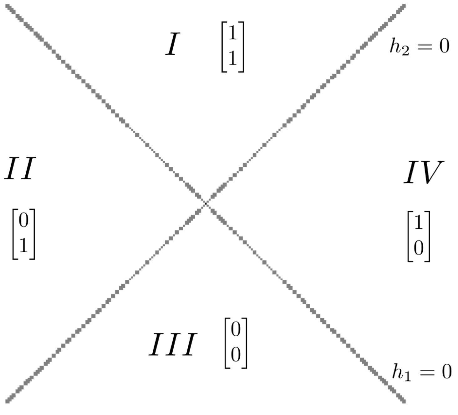
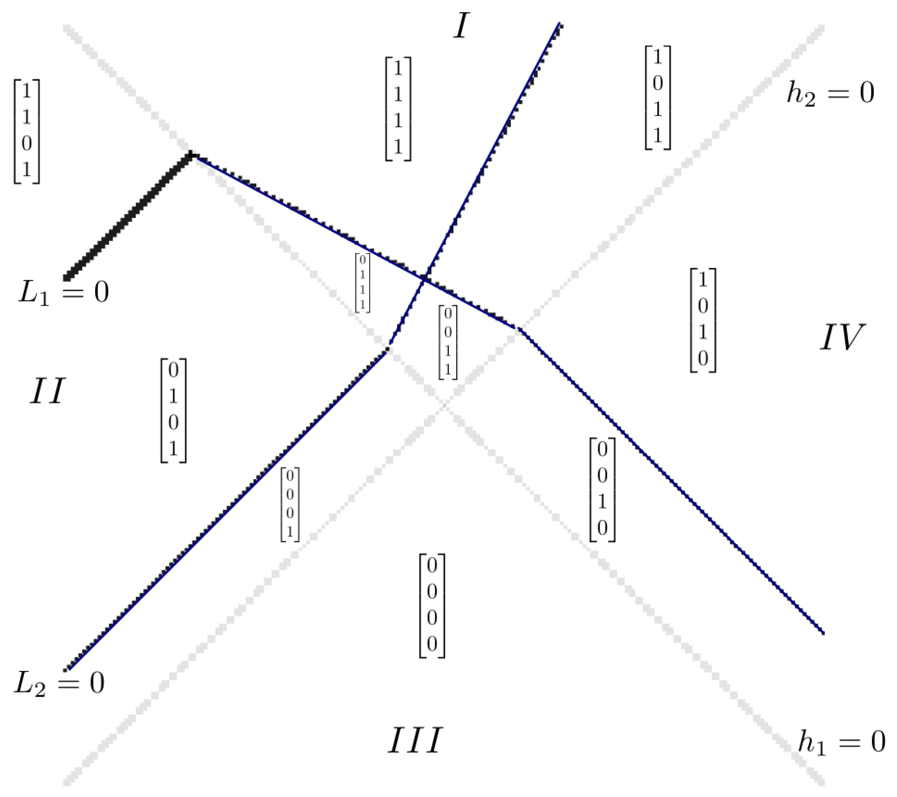
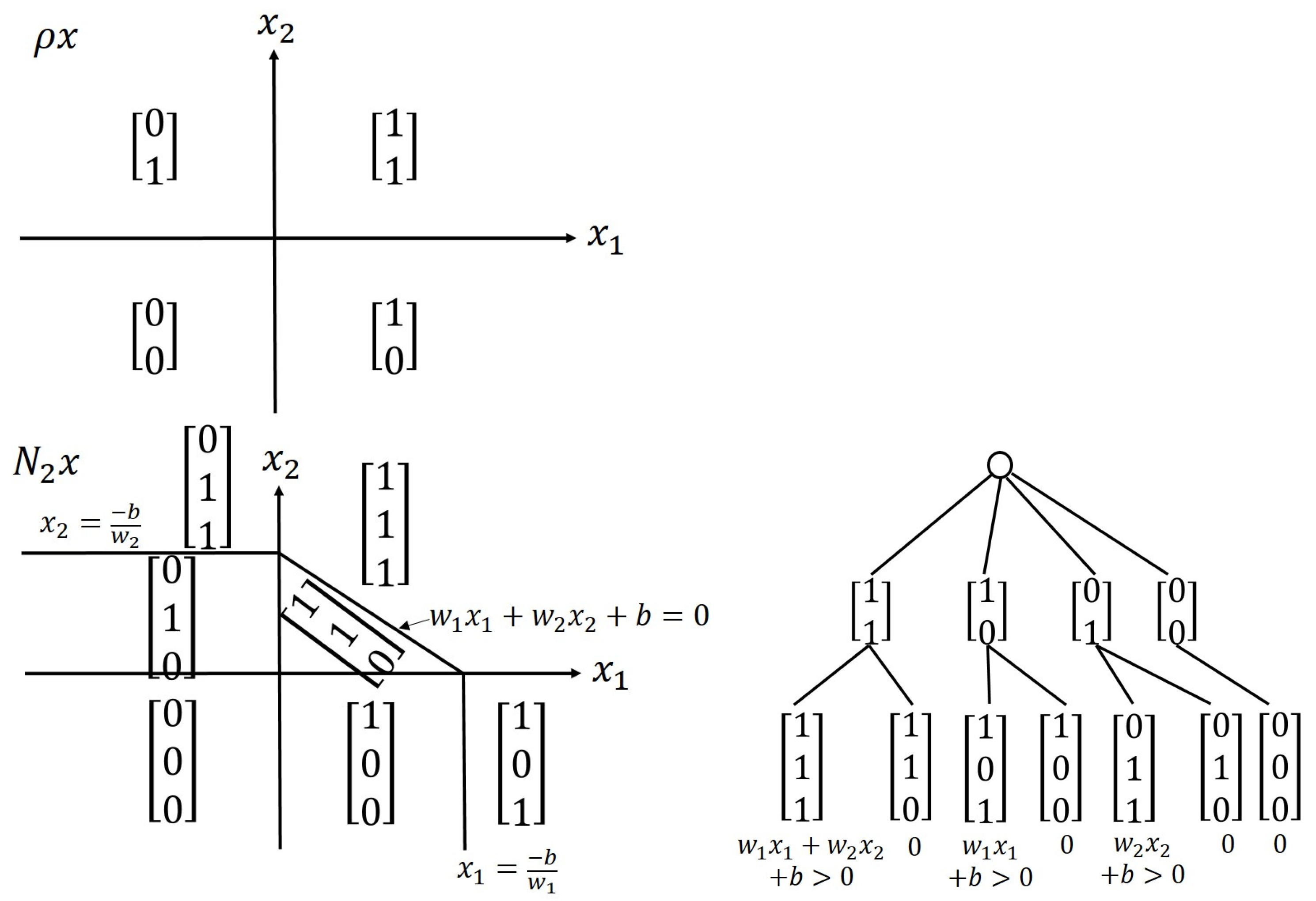
The affine linear mappings of ${\mathcal{N}}_L^s={\mathit{ReLU}}_L{M}_L{\mathcal{N}}_{L-1}^s$ can be expressed as ${\mathbb{A}}_L\chi ={\mathbf{D}}^L{M}_L{\mathbb{A}}_{L-1}\chi$, where ${\mathbf{D}}^L$ is an un-rectifying matrix of ReLU${}_L$. This means that if ${\mathbf{A}}_{L,i}\in {\mathbb{A}}_L$, then there must be a j in which $P_{L,i}\subseteq P_{L-1,j}$, such that ${\mathbf{A}}_{L,i}{P}_{L,i}={\mathbf{D}}^{L,i}{M}_L{\mathbf{A}}_{L-1,j}{P}_{L,i}$, where the un-rectifying matrix (${\mathbf{D}}^{L,i}$) depends on $M_L{\mathbf{A}}_{L-1,j}{P}_{L,i}$.

${\mathbb{P}}_L$ refines ${\mathbb{P}}_{L-1}$ (i.e., ${\mathbb{P}}_L\subseteq {\mathbb{P}}_{L-1}$), which means that if a directed graph is based on the partition refinement in the leftmost subfigure of Figure 6, then the node corresponding to ${\mathbb{P}}_L$ is the only child node of node ${\mathbb{P}}_{L-1}$, as well as the only parent node of node ${\mathbb{P}}_L$. The graph of this module is a tree with precisely one child at each node.

(3) Parallel module (Figure 7a): This module is a composition comprising an element in $\mathcal{K}$ to each output of the duplication operation, denoted as follows:

$$\begin{array}{c}\hfill \left(\mathrm{parallel}\right)\doteq \mathcal{K}\circ \left(\mathrm{duplication}\right).\end{array}$$

When expressed in matrix form, we obtain the following:

$$\begin{array}{c}\hfill \mathbf{x}\to \left[\begin{array}{c}\mathbf{I}\\ ⋮\\ \mathbf{I}\end{array}\right]\mathbf{x}\to \left[\begin{array}{c}{k}_1\\ ⋮\\ k_m\end{array}\right]\mathbf{x}.\end{array}$$

(22)

In the literature on DNNs, this module is also referred to as a multifilter ($k_i$ is typically a filtering operation followed by an activation function) or multichannel module. If partition $\mathbb{P}$ is associated with the input (i.e., $\mathbf{x}$) in (22) and partition ${\mathbb{P}}_i$ is associated with the output of the i-th channel (i.e., $k_i\mathbf{x}$), then ${\mathbb{P}}_i$ is a refinement of $\mathbb{P}$ in accordance with (2). As shown in the middle subgraph of Figure 6, the node corresponding to ${\mathbb{P}}_i$ is a child node of the node corresponding to $\mathbb{P}$. This graph is a tree in which the node of $\mathbb{P}$ has m child nodes corresponding to partitions ${\mathbb{P}}_1,\cdots ,{\mathbb{P}}_m$.

(4) Fusion module (Figure 7b): This type of module can be used to combine different parts of a DNN and uses linear operations to fuse inputs. The module is denoted as follows:

$$\begin{array}{c}\hfill \left(\mathrm{fusion}\right)\doteq \mathbf{L}\circ \left(\mathrm{concatenation}\right).\end{array}$$

(23)

In matrix form, we obtain the following:

$$\begin{array}{c}\hfill \mathbf{x}\to \{k_1{\mathbf{x}}_1,\cdots ,k_m{\mathbf{x}}_m\}\to \mathbf{L}\left[\begin{array}{c}{k}_1{\mathbf{x}}_1\\ ⋮\\ k_m{\mathbf{x}}_m\end{array}\right].\end{array}$$

Note that a non-linear fusion can be obtained by applying a composition of $\rho M$/$\rho$ to the fusion module in which $\mathbf{L}=\mathbf{I}$.

We denote the domain partition of $\chi$ associated with the i-th channel as ${\mathbb{P}}_i=\left\{R_{i{j}_i}\right|j_i=1,\cdots n_i\}$, where $n_i$ is the number of partition regions. Partition $\mathbb{P}$ of $\chi$ generated by the fusion module can be expressed as the union of non-empty intersections of partition regions in ${\mathbb{P}}_i$ for all i, as follows:

$$\begin{array}{cc}\hfill \mathbb{P}& \doteq {\mathbb{P}}_1\cap {\mathbb{P}}_2\cap \cdots \cap {\mathbb{P}}_m\hfill \\ \hfill & ={\cup }_{j_1,\cdots ,j_m}(R_{1j_1}\cap R_{2j_2}\cdots \cap R_{m{j}_m}\ne \varnothing ).\hfill \end{array}$$

(24)

Any partition region in $\mathbb{P}$ is contained in precisely one region in any ${\mathbb{P}}_i$. In other words, $\mathbb{P}$ is a refinement of ${\mathbb{P}}_i$ for $i=1,\cdots ,m$. An obvious bound for partition regions of $\mathbb{P}$ is ${\prod }_{i=1}^m{n}_i$. We let $\left\{A_{i{j}_i}\right|j_i=1\cdots n_i\}$ denote the affine mappings associated with the i-th channel and $A_{i{j}_i}$ be the affine mapping with the domain restricted to partition region $R_{i{j}_i}$. The affine mapping of the fusion module over partition region $R_{1j_1}\cap R_{2j_2}\cap \cdots \cap R_{m{j}_m}\ne \varnothing$ is derived as follows:

$$\begin{array}{c}\hfill R_{1j_1}\cap R_{2j_2}\cap \cdots \cap R_{m{j}_m}\ne \varnothing \to \mathbf{L}\left[\begin{array}{c}{A}_{1j_1}\\ ⋮\\ A_{m{j}_m}\end{array}\right].\end{array}$$

(25)

For the sake of convenience, (24) and (25) are summarized in the following lemma.

Lemma 3.

Suppose that a fusion module comprises m channels. Let ${\mathbb{P}}_i$ denote the partition associated with the i-th channel of the module and let $\mathbb{P}$ denote the partition of the fusion module. Then, $\mathbb{P}$ is a refinement of ${\mathbb{P}}_i$ for $i=1,\cdots ,m$. Moreover, let $\mathbb{A}$ denote the collection of affine linear mappings over $\mathbb{P}$. Thus, the affine linear mapping over a partition region of $\mathbb{P}$ can be obtained in accordance with (25).

As shown in the rightmost subfigure of Figure 6, $\mathbb{P}$ is a refinement of any ${\mathbb{P}}_i$, which means that the node corresponding to partition $\mathbb{P}$ is a child node of the node corresponding to partition ${\mathbb{P}}_i$. The fact that the node associated with partition $\mathbb{P}$ has more than one parent node means that the graph for this module is not a tree.

Example 2.

Figure 8 illustrates the fusion of two channels, as follows:

$$\begin{array}{c}\hfill \mathcal{M}:{\mathbb{R}}^2\to \mathbf{L}\left[\begin{array}{c}{\rho }_1{M}_1\\ {\rho }_2{M}_2\end{array}\right],\end{array}$$

where $M_1,M_2:{\mathbb{R}}^2\to {\mathbb{R}}^2$, and ${\rho }_1$ and ${\rho }_2$ are ReLUs. The partition induced by $\mathcal{M}$ comprises eight polytopes, each of which is associated with an affine linear mapping.

Figure 9 illustrates the refinement of partitions in the network in Figure 9a, which involved a series connection of five fusion layers. Each fusion layer includes a fusion module derived by a concatenation of inputs ($\mathrm{ReLU}{M}_1$ (top) and $\mathrm{ReLU}{M}_2$ (bottom)). The result of the concatenation is subsequently input into linear function $\mathbf{L}=\left[\begin{array}{cc}\mathbf{I}& \mathbf{I}\end{array}\right]$ (fusion). The curves in Figure 9b–d top–bottom respectively) and fusion channels are consistent with the assertion of Lemma 3, wherein the partitions of the top and bottom channels are refined by the fusion channel. The fusion channel is the refinement of top and bottom channels, which means that the maximum number of vectors in a given partition region and the maximum distance between pairs of points in the same partition region are smaller than in the top and bottom channels, as shown in Figure 9b,c. On the other hand, the number of partition regions in the fusion channel is larger than in the top and bottom channels, as shown in Figure 8 and Figure 9d.

(5) The following DNN networks were derived by applying the DAG closure rule (R) to the modules.

Example 3.

As shown in Figure 10, the ResNet module [11] comprises ReLU and a fusion module:

$$\begin{array}{c}\hfill \left(\mathrm{ResNet}\right)\doteq \rho \circ \left(\mathrm{fusion}\right).\end{array}$$

Using matrix notation, we obtain the following:

$$\begin{array}{c}\hfill \mathbf{x}\to \rho \left[\mathbf{I}\mathbf{I}\right]diag(\mathbf{I},-M_2\rho M_1)\left[\begin{array}{c}\mathbf{I}\\ \mathbf{I}\end{array}\right]\mathbf{x}=\rho (\mathbf{I}-M_2\rho M_1)\mathbf{x},\end{array}$$

(26)

where $M_1$ and $M_2$ are affine mappings. The unique feature of ResNet is the direct link, which enhances resistance to the gradient vanishing problem in back-propagation algorithms [29]. It is a fact that direct linking and batch normalization [30,31] have become indispensable elements in the learning of very deep neural networks using back-propagation algorithms.

Let ${\mathcal{M}}_L$ denote an L-layer DNN. A residual network [11] extends ${\mathcal{M}}_L$ from L layers to $L+2$ layers as follows: $\left(\mathit{ResNet}\right)\circ {\mathcal{M}}_L$. Repetition of this extension allows a residual network to maintain an arbitrary number of layers. As noted in the caption of Figure 10, domain partitioning is the same at a and b. This can be derived in accordance with the following analysis. Let ${\mathbb{P}}_0$ denote the domain partitioning of χ at the input of the module. The top channel of the parallel module retains the partition, whereas in the bottom channel, the partition is refined as ${\mathbb{P}}_1$ using $M_2\rho M_1$. In accordance with (24), the domain of the fusion function is ${\mathbb{P}}_1\cap {\mathbb{P}}_0$ (i.e., ${\mathbb{P}}_1$). Thus, the domain partitions at a and b are equivalent. Note that the DenseNet module [32] replaces the addition node in Figure 10 with the concatenation node. The partitions of DenseNet at b and a are the same, as in the ResNet case.

Example 4.

Transformers are used to deal with sequence-to-sequence conversions, wherein the derivation of long-term correlations between tokens in a sequence is based on the attention module [33,34]. A schematic illustration of a self-attention module is presented in Figure 11a, where the input vectors are $a^1$, $a^2$, $a^3$, and $a^4$ and outputs vectors are $b^1$, $b^2$, $b^3$, and $b^4$. The query, key, and value vectors for $a^i$ are generated from matrix $W^q$, $W^k$, and $W^v$, respectively, where $q^i=W^q{a}^i$, $k^i=W^k{a}^i$, and $v^i=W^v{a}^i$ for all i. Attention score ${\alpha }_{i,j}$ indicates the inner product between the normalized vectors of $q^i$ and $k^j$. The vector of attention scores $[{\alpha }_{i,1}$, ${\alpha }_{i,2}$, ${\alpha }_{i,3}$, and ${\alpha }_{i,4}{]}^{\top }$ are input into the soft-max layer to obtain probability distribution $[{\widehat{\alpha }}_{i,1}$, ${\widehat{\alpha }}_{i,2}$, ${\widehat{\alpha }}_{i,3}$, ${\widehat{\alpha }}_{i,4}{]}^{\top }$, where ${\widehat{\alpha }}_{i,j}=\frac{e^{{\alpha }_{i,j}}}{{\sum }_j{e}^{{\alpha }_{i,j}}}$. Output vector $b^i={\sum }_j{\widehat{\alpha }}_{i,j}{v}^j$ is derived via multiplications and additions as a linear combination of value vectors with coefficients derived from the probability distribution. Figure 11b presents a graphical representation of (a), wherein non-linear transformation σ is the soft-max function. Dictionary V of value vectors can be obtained by performing a concatenation operation, which implicitly involves reshaping the dimensions of the resulting vector to the matrix (see dashed box in the figure).

Example 5.

Figure 12 illustrates the well-known LeNet-5 network [35]. Figure 12a presents a block diagram of the network in which the input is an image ($28\times 28$ px) and the output is ten classes of characters (0 to 9). CNN block number 1 is a convolution layer with the following parameters: filter size, $5\times 5$; stride, 1; padding, 2; and six-channel output, six $28\times 28$ images. Block numbers 2 and 3 indicate MaxLU operations and six-channel output (six $14\times 14$ images). Black circle 4 indicates a concatenation operation (O2), the output of which is an image. Block number 5 indicates a convolution layer with the following parameters: filter size, $5\times 5$; stride, 1; and padding, 0. This layer outputs sixteen $10\times 10$ images. Block numbers 6 and 7 indicate MaxLU operations, the output of which is sixteen $5\times 5$ images. Black circle 8 indicates a concatenation operation (O2), the output of which is a vector. Block number 9 indicates a fully connected network with input dimensions of 400 and output dimensions of 120. Block number 10 indicates a ReLU activation function. Block number 11 is a fully connected network with an input dimension of 120 and an output dimension of 84. Block number 12 indicates a ReLU activation function. Block number 13 indicates a fully connected network with an input dimension of 84, where the output is a prediction that includes 1 of the 10 classes. Figure 12b presents a graphical representation of (a), and (c) presents a simplified graphical representation of (a). In Figure 12c, we can see that LeNet-5 begins with a sequence of compositions of modules (featuring a parallel module followed by a fusion module), then a sequence of MaxLU layers. Here, we apply the LeNet-5 network to the MNIST dataset (not limited to other datasets) with $60,000$ images. This is a simple implementation illustrating the proposed approach. Figure 13 illustrates the properties of partitions at the outputs of levels 3, 4, 7, and 8 in Figure 12b. The curves in Figure 13a–c are consistent with the assertion of Lemma 3, which indicates that the partitions of the previous channels are refined by the fusion channel. The results are similar to those in Figure 9.

Remark 1.

Graphs corresponding to partitions generated by series and parallel modules are trees. Accordingly, the partitions created by a network comprising only series and parallel modules also from a tree. According to [36], trees learned for regression or classification purposes suffer from overfitting due to the bias–variance tradeoff dilemma. However, in [37,38], it was reported that this tradeoff is not an over-riding concern (referred to as benign overfitting) when learning a deep neural network in which the number of parameters exceeds the training data by a sufficient margin. This suggests that benign overfitting is relevant to the fusion module, considering that the graph for the module is not a tree.

4. Properties of General DNNs

In accordance with the axiomatic approach, we define general DNNs (i.e., $\mathcal{K}$) as those that can be represented using DAGs. In the following, we outline the properties belonging to all members in the class.

4.1. Function Approximation via Partition Refinement

We define the computable subgraph of node a as the subgraph of the DAG containing precisely all the paths from the input node of the DAG to node a. Clearly, the computable subgraph defines a general DNN, the output node of which is a, such that it computes a CPWL function. In Figure 14a, the computable subgraph of node a (highlighted in light blue) contains node numbers 0, 1, 2, 3, and 4. The computable subgraph of node c (highlighted in light green) is contained in the subgraph of a.

In the following, we outline the domain refinement of a general DNN. Specifically, if node b is contained in a computable subgraph of a, then the domain partition imposed by that subgraph is a refinement of the partition imposed by the computable subgraph of b.

Theorem 1.

The domain partitions imposed by computable subgraphs ${\mathcal{G}}^a$ (at node a) and ${\mathcal{G}}^b$ (at node b) of a general DNN are denoted as ${\mathbb{P}}_a$ and ${\mathbb{P}}_b$, respectively. Suppose that node b is contained in subgraph ${\mathcal{G}}^a$. This means that ${\mathbb{P}}_a$ refines ${\mathbb{P}}_b$.

Proof. 

Without a loss of generality, we suppose that arcs in the general DNN are atomic operations and that the functions applied to arcs are included in base set $\mathcal{B}$. Furthermore, we suppose that p is a path from the input node to node a, which also passes through node b. $p^{\prime }$ denotes the subpath of p from node b to node a ($p^{\prime }:b=c_0\to c_1\cdots \to a=c_n$). ${\mathbb{P}}_{c_i}$ denotes the partition of input space $\chi$ defined using the computable subgraph at node $c_i$. In the following, we demonstrate that if $c_i\to c_{i+1}$, then ${\mathbb{P}}_{c_i}$ is refined by ${\mathbb{P}}_{c_{i+1}}$. Note that arc $c_i\to c_{i+1}$ belongs to one of the three atomic operations. If it is a series-connection operation (O1), then the refinement can be obtained by referring to Lemma 2. If it is a concatenation operation (O2), then the refinement is obtained by referring to Lemma 3. If it is a duplication operation (O3), then the partitions for nodes $c_i$ and $c_{i+1}$ are the same. Thus, ${\mathbb{P}}_a$ is a refinement of ${\mathbb{P}}_b$. □

Figure 14a presents the DAG representation of a DNN. Node b is contained in the computable subgraph of node a, whereas node c is contained in the computable sub-graph of b such that the domain partition of a is a refinement of the partition of b, and the domain partition of b is a refinement of the partition of c. Thus, the domain partition of node a is a refinement of the domain partition of node c.

As hinted in Theorem 1, general DNNs are implemented using a data-driven “divide and conquer” strategy when performing function approximation. In other words, when traveling a path from the input node to a node of the DNN, we can envision the progressive refinement of the input space partition along the path, where each partition region is associated with an affine linear mapping. Thus, computing a function using a general DNN is equivalent to approximating the function using local simple mappings over regions in a partition derived using the DNN. A finer approximation of the function can be obtained by increasing the lengths of paths from the input node to the output node. Figure 15 illustrates the conventional and general DNN approaches to the problem of linear regression. The conventional approach involves fitting “all” of the data to obtain a dashed hyperplane, whereas the general DNN approach involves dividing the input space into two parts and fitting each part using hyperplanes.

4.2. Stability via Sparse/Compressible Weight Coefficients

We introduce the l function of node a to denote the number of arcs along the longest path from input node I to node a of a DAG, where $l\left(a\right)$ is referred as the level of node a. According to this definition, the level of the input node is zero.

Lemma 4.

The level is a continuous integer across the nodes in a general DNN. In other words, if node a is not the output node, then there must exist a node b where $l\left(b\right)=l\left(a\right)+1$.

Proof. 

Clearly, $l\left(I\right)=0$ for input node I. This lemma can be proven via contradiction. Suppose that the levels are non-continuous integers. Without a loss of generality, the nodes can be divided into two groups (A and B), where A includes all of the nodes with level $\le n$ and B includes all of the nodes with level $\ge n+k$ and $k>1$. $b\in B$ is assigned the lowest level in graph B, and $l\left(b\right)=n+k$. Furthermore, $p\left(b\right)$ denotes the longest path from the input node to node b, and a is a node along the path with arc $a\to b$. Thus, $l\left(a\right)<n+k$; otherwise, $l\left(b\right)\ge n+k+1$, which violates the assumption that $l\left(b\right)=n+k$. If $l\left(a\right)\le n$, then $l\left(b\right)\le n+1$ (since a is on the longest path ($p\left(b\right)$) to b and a has a direct link to b). This violates the assumption that $l\left(b\right)=n+k$ with $k>1$. Thus, $n<l\left(a\right)<n+k$, according to which $a\notin A$ and $a\notin B$. This violates the assumption that all nodes can be divided into two groups (A and B). We obtain a contradiction and, hence, complete the proof. □

The nodes in a DAG can be ordered in accordance with the levels. Assume that there is only one output node, denoted as O. Clearly, $l\left(O\right)=L$ is the highest level associated with that DAG. The above lemma implies that the nodes can be partitioned into levels from 0 to L. We introduce notation $\overline{l}\left(n\right)$ (referring to the nodes at level n) to denote the collection of nodes with levels equal to n and let $|\overline{l}\left(n\right)|$ denote the number of nodes at that level. As shown in Figure 14b, the nodes in Figure 14a are ordered in accordance with their levels, as indicated by the number besides the nodes. For any DNN (${\mathcal{N}}_L\in \mathcal{K}$), we can define DNN function ${\mathcal{N}}_n$ (with $n\le L$) by stacking the DNN functions of nodes at level n into a vector as follows:

$$\begin{array}{c}\hfill {\mathcal{N}}_n={\left[{\mathcal{N}}_{\left(a\right)}\right]}_{a\in \overline{l}\left(n\right)}\end{array}$$

(27)

where $N_{\left(a\right)}$ is the function derived using the computable subgraph of node $a\in \overline{l}\left(n\right)$. Clearly, ${\mathcal{N}}_n\in \mathcal{K}$ because it is formed by the concatenation of ${\mathcal{N}}_{\left(a\right)}$. For example, in Figure 14b, ${\mathcal{N}}_3=\left[{\mathcal{N}}_{\left(b\right)}\right]$ and ${\mathcal{N}}_5=\left[\begin{array}{c}{\mathcal{N}}_{\left(s\right)}\\ {\mathcal{N}}_{\left(t\right)}\end{array}\right]$. The order of components in $N_n$ is irrelevant to subsequent analysis of stability conditions.

The stability of a DNN can be measured as the output perturbation against the input perturbation such that

$$\begin{array}{c}\hfill \parallel {\mathcal{N}}_L\left(\mathbf{x}\right)-{\mathcal{N}}_L{\left(\mathbf{y}\right)\parallel }_2\le C\left(L\right){\parallel \mathbf{x}-\mathbf{y}\parallel }_2,\end{array}$$

(28)

where L is the level of the output node for DNN ${\mathcal{N}}_L$. A stable deep architecture implies that a deep forward inference is well-posed and robust in noisy environments. A sufficient condition for the stability of a DNN requires that $C\left(L\right)$ be a bounded, non-increasing function of L when $L\to \infty$.

Lemma 5.

Let d be the uniform bound defined in (21), $I_a=\left\{b\right|b\to a\}$ (the nodes directly linking to the node a), and $|I_a|$ denote the number of nodes in $I_a$. Further, let ${\mathcal{N}}_L\in \mathcal{K}$ and ${\mathcal{N}}_{L,\mathit{p}}$ denote the restriction of ${\mathcal{N}}_L$ over partition region $\mathit{p}$. Suppose that ${\mathcal{N}}_{\left(a\right)}$ and ${\mathcal{N}}_{\left(a\right),p}$ denote the CPWL function associated with the computable subgraph of node a and the restriction of the function over $\mathit{p}$, respectively. As defined in (27), ${\mathcal{N}}_n$ denotes the function derived by nodes at level $n\le L$, and ${\mathcal{N}}_{n,\mathit{p}}$ denotes the restriction of ${\mathcal{N}}_n$ on domain partition $\mathit{p}$; i.e.,

$$\begin{array}{c}\hfill {\mathcal{N}}_{n,\mathit{p}}={\left[{\mathcal{N}}_{\left(a\right),\mathit{p}}\right]}_{a\in \overline{l}\left(n\right)}.\end{array}$$

(29)

(i) For a given n and $\mathit{p}$, there exists $C(n,p)$ such that for any $\mathbf{x},\mathbf{y}\in \mathit{p}$,

$$\begin{array}{c}\hfill \parallel {\mathcal{N}}_{n,\mathit{p}}\left(\mathbf{x}\right)-{\mathcal{N}}_{n,\mathit{p}}{\left(\mathbf{y}\right)\parallel }_2\le C(n,\mathit{p}){\parallel \mathbf{x}-\mathbf{y}\parallel }_2,\end{array}$$

(30)

where $C(n,\mathit{p})$ is referred to as the Lipschitz constant in $\mathit{p}$ at level n.

(ii) If there exists level m such that for $n\ge m$,

$$\begin{array}{c}\hfill d\sum _{a\in \overline{l}\left(n\right)}\sum _{b\in I_a}{\parallel {\mathbf{W}}_{ab}\parallel }_2\le 1,\end{array}$$

(31)

where ${\mathbf{W}}_{ab}$ is the weight matrix associated with the atomic operation on arc $a\leftarrow b$, which means that the Lipschitz constant $C(n,\mathit{p})$ is a bounded function of n on $\mathit{p}$.

Proof. 

See Appendix A for the proof. □

This lemma establishes local stability in a partition region of a DNN. To achieve global stability in the input space, we invoke the lemma in [5], which indicates that piece-wise functions that maintain local stability have global stability, provided that the functions are piece-wise continuous.

Lemma 6

([5]). Let $\chi ={\cup }_i{P}_i$ be a partition and $f_i$ with domain $\overline{P_i}$ be $l_i$-Lipschitz continuous with $f_i\left(\mathbf{x}\right)=f_j\left(\mathbf{x}\right)$ for $\mathbf{x}\in \overline{P_i}\cap \overline{P_j}$. Let f be defined by $f\left(\mathbf{x}\right):=f_i\left(\mathbf{x}\right)$ for $\mathbf{x}\in P_i$. Then, f is $\left({max}_i{l}_i\right)$-Lipschitz continuous.

Theorem 2.

For the sake of stability, we adopted the assumption pertaining to Lemma 5. Let DNN ${\mathcal{N}}_L\in \mathcal{K}$ with the domain in input space (χ) and let ${\mathcal{N}}_n$ denote the function with nodes of ${\mathcal{N}}_L$ up to level $n\le L$. If there exists level m such that for $n\ge m$,

$$\begin{array}{c}\hfill d\sum _{a\in \overline{l}\left(n\right)}\sum _{b\in I_a}{\parallel {\mathbf{W}}_{ab}\parallel }_2\le 1\end{array}$$

(32)

where d is the uniform bound defined in (21), and ${\mathbf{W}}_{ab}$ is the weight matrix associated with arc $a\leftarrow b$; then, for any partitioning region p of χ, $C\left(L\right)={max}_{\mathit{p}}C(L,\mathit{p})$ is a bounded, non-increasing function of L on χ. Note that $C\left(L\right)$ is defined in (28). Hence, ${\mathcal{N}}_L$ is a stable architecture.

Proof. 

See Appendix B for the proof. □

This theorem extends the stability of the series-connected DNNs in [5] to general DNNs. According to ${\parallel \mathbf{W}\parallel }_F\ge {\parallel \mathbf{W}\parallel }_2$, the condition determining the stability of an DNN can be expressed as follows:

$$\begin{array}{c}\hfill d\sum _{a\in \overline{l}\left(n\right)}\sum _{b\in I_a}{\parallel {\mathbf{W}}_{ab}\parallel }_F\le 1.\end{array}$$

(33)

This condition holds, regardless of the size of ${\mathbf{W}}_{ab}$. Thus, if the matrix is large, then (33) implies that the weight coefficients are sparse/compressible. Note that (32) is a sufficient condition for a DNN to achieve stability; however, it is not a necessary condition. The example in Figure 16 demonstrates that satisfying (32) is not necessary.

Figure 17 illustrates simulations pertaining to Theorem 2 for the network presented in Figure 9a, which comprises a fusion module with five layers. The simulations illustrate how the weight coefficients affect the Lipschitz constant. In Figure 17a, the upper bound for Lipschitz constant $C\left(L\right)$, where $L=1,\cdots ,5$ (presented as the maximum gain $\parallel {\mathcal{N}}_L\mathbf{x}-{\mathcal{N}}_L{\mathbf{y}\parallel }_2/{\parallel \mathbf{x}-\mathbf{y}\parallel }_2$ for all pairs of training data), increases with an increase in the number of fusion layers if the weight coefficients do not satisfy (32) in terms of stability. If the weight coefficients were scaled to be compressible in accordance with (32), then the upper bound would decrease with an increase in the number of fusion layers, as shown in Figure 17b. This is an indication that the network is stable relative to the input perturbation.

5. Conclusions

Using an axiomatic approach, we established a systematic approach to representing deep feedforward neural networks (DNNs) as directed acyclic graphs (DAGs). The class of DNNs constructed using this approach is referred to as general DNNs, which includes DNNs with pragmatic modules, activation functions, and non-linear transformations. We demonstrated that general DNNs approximate a target function in a coarse-to-fine manner by learning a directed graph (generally not in a tree configuration) through the refinement of input space partitions. Furthermore, if the weight coefficients become increasingly sparse along any path of a graph, then the DNN function gains stability with respect to perturbations in the input space due to a bounded global Lipschitz constant. This study provides a systematic approach to studying a wide range of DNNs with architectures that are more complex than those of simple series-connected DNN models. In the future, we will explore the analysis and conclusions reported in this paper in terms of their applications. In this direction, we refer to [39] with respect to network pruning.

References

- Yang, Y.; Sun, J.; Li, H.; Xu, Z. Deep ADMM-Net for compressive sensing MRI. In Advances in Neural Information Processing Systems; Curran Associates, Inc.: Red Hook, NY, USA, 2016; Volume 29. [Google Scholar]
- Monga, V.; Li, Y.; Eldar, Y.C. Algorithm unrolling: Interpretable, efficient deep learning for signal and image processing. IEEE Signal Process. Mag. 2021, 38, 18–44. [Google Scholar] [CrossRef]
- Molnar, C. Interpretable Machine Learning. Lulu.com. 2020. Available online: https://christophmolnar.com/books/interpretable-machine-learning/ (accessed on 9 September 2023).
- Balestriero, R.; Cosentino, R.; Aazhang, B.; Baraniuk, R. The Geometry of Deep Networks: Power Diagram Subdivision. In Advances in Neural Information Processing Systems; Curran Associates, Inc.: Red Hook, NY, USA, 2019; pp. 15806–15815. [Google Scholar]
- Hwang, W.L.; Heinecke, A. Un-rectifying non-linear networks for signal representation. IEEE Trans. Signal Process. 2019, 68, 196–210. [Google Scholar] [CrossRef]
- Li, Q.; Lin, T.; Shen, Z. Deep learning via dynamical systems: An approximation perspective. arXiv 2019, arXiv:1912.10382. [Google Scholar] [CrossRef]
- Baraniuk, R. The local geometry of deep learning (Power Pointer slides). In Proceedings of the 2023 IEEE International Conference on Acoustics, Speech and Signal Processing (Plentary Speech), Rhodes Island, Greece, 4–10 June 2023. [Google Scholar]
- Sun, W.; Tsiourvas, A. Learning Prescriptive ReLU Networks. arXiv 2023, arXiv:2306.00651. [Google Scholar]
- Kipf, T.N.; Welling, M. Semi-supervised classification with graph convolutional networks. arXiv 2016, arXiv:1609.02907. [Google Scholar]
- Duvenaud, D.; Maclaurin, D.; Aguilera-Iparraguirre, J.; Gómez-Bombarelli, R.; Hirzel, T.; Aspuru-Guzik, A.; Adams, R.P. Convolutional networks on graphs for learning molecular fingerprints. arXiv 2015, arXiv:1509.09292. [Google Scholar]
- He, K.; Zhang, X.; Ren, S.; Sun, J. Deep residual learning for image recognition. In Proceedings of the IEEE Conference on Computer Vision and Pattern Recognition, Las Vegas, NV, USA, 27–30 June 2016; pp. 770–778. [Google Scholar]
- Weinan, E. A proposal on machine learning via dynamical systems. Commun. Math. Stat. 2017, 1, 1–11. [Google Scholar]
- Lu, Y.; Zhong, A.; Li, Q.; Dong, B. Beyond finite layer neural networks: Bridging deep architectures and numerical differential equations. In Proceedings of the International Conference on Machine Learning, Stockholm, Sweden, 10–15 July 2018; pp. 3276–3285. [Google Scholar]
- Haber, E.; Ruthotto, L. Stable architectures for deep neural networks. Inverse Probl. 2017, 34, 014004. [Google Scholar] [CrossRef]
- Chang, B.; Chen, M.; Haber, E.; Chi, E.H. AntisymmetricRNN: A dynamical system view on recurrent neural networks. arXiv 2019, arXiv:1902.09689. [Google Scholar]
- Ascher, U.M.; Petzold, L.R. Computer Methods for Ordinary Differential Equations and Differential-Algebraic Equations; SIAM: Philadelphia, PA, USA, 1998; Volume 61. [Google Scholar]
- Mallat, S. Group invariant scattering. Commun. Pure Appl. Math. 2012, 65, 1331–1398. [Google Scholar] [CrossRef]
- Bruna, J.; Mallat, S. Invariant scattering convolution networks. IEEE Trans. Pattern Anal. Mach. Intell. 2013, 35, 1872–1886. [Google Scholar] [CrossRef] [PubMed]
- Kuo, C.C.J.; Chen, Y. On data-driven saak transform. J. Vis. Commun. Image Represent. 2018, 50, 237–246. [Google Scholar]
- Gregor, K.; LeCun, Y. Learning fast approximations of sparse coding. In Proceedings of the 27th International Conference on International Conference on Machine Learning, Haifa, Israel, 21–24 June 2010; pp. 399–406. [Google Scholar]
- Zhang, J.; Ghanem, B. ISTA-Net: Interpretable optimization-inspired deep network for image compressive sensing. In Proceedings of the IEEE Conference on Computer Vision and Pattern Recognition, Salt Lake City, UT, USA, 18–22 June 2018; pp. 1828–1837. [Google Scholar]
- Chan, S.H. Performance analysis of plug-and-play ADMM: A graph signal processing perspective. IEEE Trans. Comput. Imaging 2019, 5, 274–286. [Google Scholar] [CrossRef]
- Heinecke, A.; Ho, J.; Hwang, W.L. Refinement and universal approximation via sparsely connected ReLU convolution nets. IEEE Signal Process. Lett. 2020, 27, 1175–1179. [Google Scholar] [CrossRef]
- Arora, R.; Basu, A.; Mianjy, P.; Mukherjee, A. Understanding deep neural networks with rectified linear units. arXiv 2016, arXiv:1611.01491. [Google Scholar]
- Goodfellow, I.; Warde-Farley, D.; Mirza, M.; Courville, A.; Bengio, Y. Maxout networks. In Proceedings of the International Conference on Machine Learning, Atlanta, GA, USA, 16–21 June 2013; pp. 1319–1327. [Google Scholar]
- Krizhevsky, A.; Sutskever, I.; Hinton, G.E. Imagenet classification with deep convolutional neural networks. In Advances in Neural Information Processing Systems; Curran Associates, Inc.: Red Hook, NY, USA, 2012; Volume 25. [Google Scholar]
- Gao, B.; Pavel, L. On the properties of the softmax function with application in game theory and reinforcement learning. arXiv 2017, arXiv:1704.00805. [Google Scholar]
- Goodfellow, I.; Bengio, Y.; Courville, A. Deep Learning; MIT Press: Cambridge, MA, USA, 2016. [Google Scholar]
- Kingma, D.P.; Ba, J. Adam: A method for stochastic optimization. arXiv 2014, arXiv:1412.6980. [Google Scholar]
- Ioffe, S.; Szegedy, C. Batch normalization: Accelerating deep network training by reducing internal covariate shift. arXiv 2015, arXiv:1502.03167. [Google Scholar]
- Szegedy, C.; Ioffe, S.; Vanhoucke, V.; Alemi, A.A. Inception-v4, inception-resnet and the impact of residual connections on learning. In Proceedings of the Thirty-First AAAI Conference on Artificial Intelligence, San Francisco, CA, USA, 4–9 February 2017. [Google Scholar]
- Huang, G.; Liu, Z.; Van Der Maaten, L.; Weinberger, K.Q. Densely connected convolutional networks. In Proceedings of the IEEE Conference on Computer Vision and Pattern Recognition, Honolulu, HI, USA, 21–26 July 2017; pp. 4700–4708. [Google Scholar]
- Vaswani, A.; Shazeer, N.; Parmar, N.; Uszkoreit, J.; Jones, L.; Gomez, A.N.; Kaiser, Ł.; Polosukhin, I. Attention is all you need. In Advances in Neural Information Processing Systems; Curran Associates, Inc.: Red Hook, NY, USA, 2017; Volume 30. [Google Scholar]
- Dosovitskiy, A.; Beyer, L.; Kolesnikov, A.; Weissenborn, D.; Zhai, X.; Unterthiner, T.; Dehghani, M.; Minderer, M.; Heigold, G.; Gelly, S.; et al. An image is worth 16x16 words: Transformers for image recognition at scale. arXiv 2020, arXiv:2010.11929. [Google Scholar]
- LeCun, Y.; Bottou, L.; Bengio, Y.; Haffner, P. Gradient-based learning applied to document recognition. Proc. IEEE 1998, 86, 2278–2324. [Google Scholar] [CrossRef]
- Geman, S.; Bienenstock, E.; Doursat, R. Neural networks and the bias/variance dilemma. Neural Comput. 1992, 4, 1–58. [Google Scholar] [CrossRef]
- Belkin, M.; Hsu, D.; Ma, S.; Mandal, S. Reconciling modern machine-learning practice and the classical bias–variance trade-off. Proc. Natl. Acad. Sci. USA 2019, 116, 15849–15854. [Google Scholar] [CrossRef] [PubMed]
- Cao, Y.; Chen, Z.; Belkin, M.; Gu, Q. Benign overfitting in two-layer convolutional neural networks. In Advances in Neural Information Processing Systems; Curran Associates, Inc.: Red Hook, NY, USA, 2022; Volume 35, pp. 25237–25250. [Google Scholar]
- Hwang, W.L. Representation and decomposition of functions in DAG-DNNs and structural network pruning. arXiv 2023, arXiv:2306.09707. [Google Scholar]
Disclaimer/Publisher’s Note: The statements, opinions and data contained in all publications are solely those of the individual author(s) and contributor(s) and not of MDPI and/or the editor(s). MDPI and/or the editor(s) disclaim responsibility for any injury to people or property resulting from any ideas, methods, instructions or products referred to in the content. |
© 2023 by the authors. Licensee MDPI, Basel, Switzerland. This article is an open access article distributed under the terms and conditions of the Creative Commons Attribution (CC BY) license (https://creativecommons.org/licenses/by/4.0/).
Share and Cite
Hwang, W.-L.; Tung, S.-S. Analysis of Function Approximation and Stability of General DNNs in Directed Acyclic Graphs Using Un-Rectifying Analysis. Electronics 2023, 12, 3858. https://doi.org/10.3390/electronics12183858
Hwang W-L, Tung S-S. Analysis of Function Approximation and Stability of General DNNs in Directed Acyclic Graphs Using Un-Rectifying Analysis. Electronics. 2023; 12(18):3858. https://doi.org/10.3390/electronics12183858
Chicago/Turabian StyleHwang, Wen-Liang, and Shih-Shuo Tung. 2023. "Analysis of Function Approximation and Stability of General DNNs in Directed Acyclic Graphs Using Un-Rectifying Analysis" Electronics 12, no. 18: 3858. https://doi.org/10.3390/electronics12183858
APA StyleHwang, W.-L., & Tung, S.-S. (2023). Analysis of Function Approximation and Stability of General DNNs in Directed Acyclic Graphs Using Un-Rectifying Analysis. Electronics, 12(18), 3858. https://doi.org/10.3390/electronics12183858