Predicting Software Defects in Hybrid MPI and OpenMP Parallel Programs Using Machine Learning

Abstract

High-performance computing (HPC) and its supercomputers are essential for solving the most difficult issues in many scientific computing domains. The proliferation of computational resources utilized by HPC systems has resulted in an increase in the associated error rates. As such, modern HPC systems promote a hybrid programming style that integrates the message-passing interface (MPI) and open multi-processing (OpenMP). However, this integration often leads to complex defects, such as deadlocks and race conditions, that are challenging to detect and resolve. This paper presents a novel approach: using machine learning algorithms to predict defects in C++-based systems by employing hybrid MPI and OpenMP models. We focus on employing a balanced dataset to enhance prediction accuracy and reliability. Our study highlights the effectiveness of the support vector machine (SVM) classifier, enhanced with term frequency (TF) and recursive feature elimination (RFE) techniques, which demonstrates superior accuracy and performance in defect prediction when compared to other classifiers. This research contributes significantly to the field by providing a robust method for early defect detection in hybrid programming environments, thereby reducing development time, costs and improving the overall reliability of HPC systems.

1. Introduction

The reliability and quality of software generally depend on the elimination of errors or defects in the software. While some defects occur for reasons unrelated to the code, such as compiler or bytecode representation, the main cause of software defects is the software code itself.

The IEEE standard defines a software defect (SD) as “an imperfection or deficiency in a work product where that work product does not meet its requirements or specifications and needs to be either repaired or replaced” [1]. Software defect prediction (SDP) techniques aim to identify potential defects and faults in the software, and they represent a promising approach to improving software quality. Applying the SDP model early in the software lifecycle allows practitioners to focus more on modules than on the other modules of the software system, thereby enabling those modules to be identified as “error-prone” [2]. This reduces development costs and minimizes maintenance efforts.

SDP models classify source code modules based on the features used to represent them [3]. Various methods have been developed using SDP techniques to improve software quality and reduce baseline costs. This is achieved by predicting a faulty part of the code [4,5,6]. However, testing and code reviews can be focused on defect-prone parts once identified. For that reason, SDP studies are of great practical importance as they increase attention and productivity for software quality management [7]. The traditional approach to finding software defects is through testing and conducting reviews. These activities may require extensive effort and time. However, employing automated prediction to identify defective modules at an early stage can empower developers to achieve superior code quality at a lower cost compared to manual approaches [8].

Nowadays, high-performance computing (HPC) plays a crucial and influential role in advancing cutting-edge areas of research, supporting innovation, and facilitating the development of applications in various industries. Standard programming languages cannot handle parallelism effectively, so alternative programming models have been developed to make it easier to write parallel programs. These programming models can be integrated into standard programming languages, such as C, C++, Python, Java, and Fortran, to give them the ability to run parallel tasks. The integration of C++ with MPI and OpenMP has become a prominent approach in the field of HPC applications because of the demand for enhanced performance, scalability, and adaptability in parallel and distributed computing systems.

Performance and parallelism can be enhanced by integrating many programming paradigms and being able to run these on different platforms. Moreover, the utilization of hybrid programming models enhances the efficiency of achieving exa-scale computing capabilities, necessitating the development of programming models capable of effectively supporting massively parallel systems. The programming models can be categorized into three tiers: the single-level programming model, which includes MPI; the dual-level programming model, which combines MPI and OpenMP; and the tri-level programming model, which incorporates MPI, OpenMP, and CUDA [9].

However, the integration of different parallel programming models, such as MPI and OpenMP, will cause some errors, such as deadlock, lovelock, and race conditions. The process of testing parallel applications poses significant challenges due to the inherent difficulty in detecting parallel errors and the nondeterministic behavior exhibited by parallel programs, especially when a hybrid model is adopted. In addition, there needs to be more studies related to testing and detecting errors for software implemented in hybrid parallel programming models, such as MPI and OpenMP, based on machine learning (ML). Recently, the integration of artificial intelligence (AI) in software testing has been growing and may soon replace traditional manual testing methods [10]. In addition, AI-powered testing can further support decision-making, improved test coverage, faster feedback, and reduced resource allocation [11]. In the context of software defect prediction, the integration of AI has yielded favorable prediction performance [12]. Specifically, ML techniques have been employed for defect prediction by leveraging numerous feature types from source code that distinguish between defective and nondefective code, such as code size, code complexity, and process metrics [13].

In this paper, we developed a set of defect prediction models based on supervised machine learning algorithms. The proposed models effectively utilize information pertaining to errors in the source code by representing the data as tokens of the source code and feeding them as input to ML classifiers. In this study, we address the following four research questions:

Research Question 1: How do ML classifiers perform in predicting defective OpenMP and MPI code?

Research Question 2: How does feature scaling improve the prediction of defective OpenMP and MPI code?

Research Question 3: How does feature selection/reduction improve the prediction of defective OpenMP and MPI code?

Research Question 4: How does hyperparameter tuning improve the prediction of defective OpenMP and MPI code?

The novelty of our study is expressed by its contributions to the area of automatically predicting defects in parallel programs from two main facets, as follows:

• First, to the best of our knowledge, it is the first study to employ machine learning to predict defects in parallel programs implemented in C++ using a hybrid model of MPI and OpenMP. Previous research has focused solely on detecting defects in MPI or OpenMP independently or has employed using static analysis techniques, which is restricted to certain predefined rule-based heuristics. Adopting ML techniques for predicting defects in parallel programs can lead to more reliable, efficient, and error-free MPI and OpenMP applications. To do so, we developed a set of systematically designed and optimized ML-based solutions for predicting defects in hybrid MPI and OpenMP programming models.
• Second, in terms of dataset, there has been no available datasets containing hybrid C++ parallel programs (defective and non-defective) that involve MPI and OpenMP directives together. Therefore, we constructed a new dataset in this context, which is also considered the largest in terms of number of defective programs with a balanced number of non-defective programs.
• We conducted a carefully validated experimentation of ML classifiers under various configurations, considering feature extraction, scaling/normalization, and selection/reduction as well as model hyperparameter tuning.

The remainder of this article is organized as follows: Section 2 briefly presents some background of the program models that were employed in this paper and their different errors with examples. Section 3 discusses related work. Section 4 presents the approach and proposed software defect prediction architecture, and Section 5 illustrates the evaluation results. Section 6 draws the discussion. Section 7 illustrated threats to validity. Finally, Section 8 concludes the paper.

2. Background

In this section, we present the basic background of MPI and OpenMP programming models and their errors.

On the way to exa-scale computing, numerous novel issues are emerging, and the precise nature of these challenges remains uncertain. It is widely acknowledged that there is a consensus regarding the anticipated increase in the number of processes, which is expected to grow by a factor ranging from 10 to 100 [14].

Multicore processors are becoming more widely available and can significantly improve performance, so more and more parallel programs are being written to take advantage of them. While parallel programs can run much faster than sequential programs, they are also more likely to contain errors because they are more complex. Rosa et al. [15] highlighted that parallel programs are more difficult to write and debug than sequential programs because they must co-ordinate the execution of multiple threads on multiple processors. This can lead to several errors, such as race conditions and deadlocks. However, testing parallel applications is challenging due to their unpredictable behavior, which makes it hard to identify parallel defects when they occur. It is difficult to determine whether these errors have been corrected or are still in hiding if they were encountered and the source code was corrected. The test process will become even more complicated if the application includes different programming models, such as a hybrid model for MPI and OpenMP.

2.1. MPI (Message-Passing Interface)

The message-passing interface (MPI) is widely recognized as the prevailing standard for distributed memory computing in the field of high-performance computing (HPC) [16]. HPC software consists of a substantial number of lines of code, exceeding hundreds of thousands. These systems employ intricate MPI communication patterns to optimize distributed computations and achieve maximum efficiency. MPI provides a set of functions, subroutines, or methods in C, C++, and Fortran for expressing communications between tasks and processes.

The MPI program follows a specific structure. In the beginning, an MPI header file (mpi.h) was included to use MPI functions. Then, the MPI environment was initialized using the MPI_Init() function, which means the beginning of the parallel code. After that, MPI communication calls are used to send and receive messages between processes. Finally, the MPI environment is terminated using the MPI_Finalize() function, which means the end of the parallel code. Figure 1 illustrates the overall structure of an MPI program.

In an MPI program, each process runs a parallel instance of a program in its own private address space and exchanges data across distributed memory systems using messages. MPI communications can be either point-to-point or collective. In point-to-point communications, only two tasks (send/recv) are involved. On the other hand, collective communications involve a group of processes, namely, broadcast, scatter, gather, and reduction.

According to the MPI standard, all processes must call blocking and nonblocking collective operations in the same order. If a process does not participate in a collective operation, it can cause unexpected behavior, such as a program defect.

MPI Errors

Erroneous arguments: This type of error relates to a single MPI call. It occurs in the following situations: when the MPI arguments are ordered incorrectly, passing invalid arguments, such as a message size of less than zero, and exceeding the specified buffer argument’s length while performing a send operation.

Deadlock occurs when two or more processes are waiting for each other to release a resource. This can happen when two processes are both trying to send a message to each other. For example, the following code snippet (Listing 1) could lead to a deadlock:

Listing 1. Example of deadlock error in MPI.

// Rank 0 sends data to Rank 1 and then waits for Rank 1 to send data back if (rank == 0) { MPI_Send(data, 10, MPI_INT, 1, 0, comm); MPI_Recv(data, 10, MPI_INT, 1, 0, comm, MPI_STATUS_IGNORE); } // Rank 1 waits for Rank 0 to send data and then sends data back to Rank 0 else if (rank == 1) { MPI_Recv(data, 10, MPI_INT, 0, 0, comm, MPI_STATUS_IGNORE); MPI_Send(data, 10, MPI_INT, 0, 0, comm); }

In the above code, Rank 0 sends data to Rank 1 and then waits for Rank 1 to send data back. Rank 1 waits for Rank 0 to send data and then sends data back to Rank 0. If both Rank 0 and Rank 1 execute their code at the same time, then a deadlock will occur because each process is waiting for the other to send data. Another scenario in which deadlock occurs in an MPI call where there are more receivers than senders; if this happens, then each process is waiting for the other process to send or receive data, but neither process is sending or receiving data.

Race condition is another type of MPI error, which occurs when two or more processes are accessing the same shared data at the same time or when several messages are sent to the same destination with the same tag number. The snippet code in Listing 2 illustrates this case:

Listing 2. Example of race condition error in MPI.

if (rank != 0) { // All processes other than rank 0 send their rank as a message to rank 0. MPI_Send(&rank, 1, MPI_INT, 0, tag, MPI_COMM_WORLD); } else { // Rank 0 (receiver) receives messages from any source. for (int i = 1; i < size; i++) { int received_rank; MPI_Status status; MPI_Recv(&received_rank, 1, MPI_INT, MPI_ANY_SOURCE, tag, MPI_COMM_WORLD, &status); std::cout << "Receiver got message from rank: " << received_rank << std::endl; } }

The key race condition aspect in the above code snippet is the use of MPI_ANY_SOURCE in the MPI_Recv call. This means the receiver (rank 0) is ready to receive messages from any sender process. As a result, the order in which rank 0 receives these messages is unpredictable, which leads to a race condition. Another error that might occur in the MPI model is “mismatch”, where the types of data sent and received do not match while the number of bytes sent is the same. Data race is another type of error that could happen in MPI calls in the situation of nonblocking calls with a single-threaded MPI program when the buffer is accessed prior to the operation being finished. An example of this scenario can be seen in Listing 3:

Listing 3. Example of data race error in MPI.

if (rank == 0) {  int send_data = 123;  MPI_Isend(&send_data, 1, MPI_INT, 1, tag, MPI_COMM_WORLD, &request); // do work  // Incorrectly modifying the buffer before the non-blocking send completes can result in a data race.  send_data = 456; } else if (rank == 1) { int recv_data;  MPI_Irecv(&recv_data, 1, MPI_INT, 0, tag, MPI_COMM_WORLD, &request); // … some code here … // Accessing the buffer before the non-blocking receive completes can also result in a data race. std::cout << "Received data (potentially incorrect due to data race): " << recv_data << std::endl; std::cout << "Received data after ensuring completion: " << recv_data << std::endl; }

In the above example (Listing 3), the nonblocking call MPI_Isend initiates a send, but this call does not block (does not wait for the send to complete). In this context, a data race is observed. The application promptly alters the send_data variable after starting a nonblocking send operation. Due to the potential continuous nature of the send operation in the background, there exists uncertainty over whether the message being transmitted includes the initial value of send_data (123) or the altered value (456). In order to solve this issue, proper synchronization with MPI_Wait can be used after each nonblocking call and before accessing or modifying the buffer. This ensures that the nonblocking operation is completed before the program continues, as illustrated in Listing 4.

Listing 4. A proper synchronization to avoid the race condition error in Listing 3.
For rank 0:	For rank 1:
MPI_Isend(&send_data, 1, MPI_INT, 1, tag, MPI_COMM_WORLD, &request); MPI_Wait(&request, MPI_STATUS_IGNORE); sent_date = 456;	MPI_Irecv(&recv_data, 1, MPI_INT, 0, tag, MPI_COMM_WORLD, &request); MPI_Wait(&request, MPI_STATUS_IGNORE);

However, the message-passing interface (MPI) possesses the capability to be seamlessly integrated with other programming models, such as OpenMP, which is associated with shared memory, and OpenACC, which is associated with GPU programming.

2.2. OpenMP (Open Multi-Processing)

OpenMP is the de facto standard for parallel programming for shared memory architectures [17]. A collective group of co-operating threads carries out the execution of an OpenMP program. The OpenMP programming model is realized through a collection of compiler directives and library functions that are specifically designed for the C/C++ and Fortran programming languages. The directives provide instructions to the compiler regarding the management and synchronization of threads, as well as the distribution of workloads. OpenMP is widely supported by several open-source and private compilers for the C/C++ and Fortran programming languages. In Figure 2, the process of creating and managing threads in OpenMP, which adheres to the fork–join paradigm, wherein a program initiates execution within a single (master) thread, is illustrated. When the master thread comes across a parallel region, it forks several threads. Once the program executes a thread join operation and continues sequential execution by using the master thread (once all threads inside the region have completed their designated tasks), OpenMP provides a range of work-sharing structures that facilitate the division of computational tasks within a parallel zone. The utilization of a loop construct enables the allocation of iterations from for-loop to be executed concurrently by the collective OpenMP threads [18].

OpenMP Errors

The OpenMP programming model has many types of errors. One of these errors is deadlock, which occurs when two or more threads are waiting for input from one another. This results in an infinite loop between these threads, preventing any of the threads from making progress. There are some situations that lead to deadlock, such as the incorrect usage of an asynchronous feature. For example, incorrectly ordering locks in OpenMP can result in a situation where multiple threads are forced to wait for one another. Listing 5 illustrates this situation.

Listing 5. Deadlock in OpenMP.

if (tid == 0) { omp_set_lock(&lockA);// Acquiring lockA first // … do work omp_set_lock(&lockB);// Then trying to acquire lockB // … } else if (tid == 1) { omp_set_lock(&lockB);// Acquiring lockB first // … do work omp_set_lock(&lockA);// Then trying to acquire lockA (incorrect use of locks) // … }

Another type of OpenMP error is the race condition, which can occur when two or more threads are accessing a shared resource and at least one of these threads executes write access. Thus, the result of an operation can change depending on the order of execution in a multi-threaded program.

In Listing 6, the shared variable var1 has been changed by multiple threads; thus, the result of var1 is determined by the thread execution order.

Listing 6. Race condition in OpenMP.

#pragma omp parallel { #pragma omp for nowait shared(val1)// shared data var1 for(i = 0; i < N; i++) { if(val1 < A[i]) val1 = A[i]; } } #pragma omp parallel { #pragma omp for nowait shared(val1)// shared data var1 for(i = 0; i < N; i++) { if(val1 < A[i]) val1 = A[i]; } }

As such, modern HPC systems promote a hybrid programming style that integrates OpenMP with MPI. However, integrating both programming paradigms at the same time can lead to more error-prone software. This paper aimed to predict software defects in a hybrid model of MPI and OpenMP implemented in C++ based on ML techniques.

2.3. Hybrid MPI-OpenMP Errors

As we transition from peta-scale to exa-scale systems, there is a growing need for the integration of MPI with shared-memory techniques, such as OpenMP, to effectively utilize the capabilities of future systems. In the hybrid model, as illustrated in Figure 3, MPI is responsible for distributing the work over the network across multiple clusters and CPUs, while OpenMP is responsible for distributing load among CPU-core-based threads, and data can be shared or made private for each thread as needed by the program.

Although OpenMP programming promises more effective use of node-level resources, its own class of defects already makes MPI programs complex. They include deadlocks brought on by the improper usage of thread-level locks for mutual exclusion or data races on shared memory. In this paper, we discuss the most applicable errors that are relevant to both the MPI process and OpenMP shared memory, such as deadlock and data race.

One of the most applicable errors in hybrid MPI and OpenMP models is deadlock. In hybrid applications, deadlock occurs when threads or processes are stuck waiting for events that will never occur, which is often due to circular dependencies or unmet synchronization conditions. In addition, deadlocks in MPI applications can be detected as either pure MPI deadlocks or pure OpenMP deadlocks, depending on whether the application is multi-thread or not. In single-threaded MPI applications, deadlocks typically occur due to the specific order in which blocking operations are performed, as we mentioned in the MPI error before. The following snippet code Listing 7 illustrates deadlock in the hybrid model.

Listing 7. Deadlock in the hybrid model.

#pragma omp single { #pragma omp task { MPI_Recv(recv_buffer, /* … */); } #pragma omp task { MPI_Send(send_buffer, /* … */); } }

In the above code Listing 7, two processes that are exchanging data using OpenMP tasks are likely to work correctly if each process has at least two threads. According to [20], this code is not compliant with the OpenMP standard, and it can deadlock regardless of how many threads you use. This means that the program must not produce different results or deadlock, depending on how the threads are scheduled.

Another type of hybrid error is race condition; this error occurs when multiple threads access and modify shared data (write access) concurrently without proper synchronization, leading to unpredictable and erroneous behavior.

In above code Listing 8, we see access to the shared variable shared_variable by both OpenMP thread 0 and MPI process 0, without any synchronization, and at least one of them is writing to it. In order to avoid this situation, a synchronization mechanism, such as a critical section or locks, is used to protect the shared variable.

Listing 8. Race condition in the hybrid model

#pragma omp parallel { // OpenMP thread 0 int shared_variable = 0; if (omp_get_thread_num() == 0) { shared_variable++; } // MPI process 0 if (omp_get_num_threads() == 1) { // … communicate with other MPI processes … // … read/write shared_variable … }}

3. Related Works

This section provides an overview of SDP research and the state-of-the-art machine learning techniques used to detect defects in sequential and parallel HPC software. Researchers have utilized various methodologies to address and mitigate the impacts of defects in the source code. When using machine learning techniques, one of the most prominent approaches focuses on defect prediction, which may help developers address these issues before they arise in a production environment.

Ji et al. [21] introduced a new weighted naive Bayes classifier to SDP. They used the concept of information diffusion to assign weights to the features used in the classifier, resulting in better prediction accuracy than traditional naive Bayes classifiers. Although the strategy appears promising, the authors’ experimental evaluation could benefit from using larger and more varied datasets to better show the method’s efficacy.

Hammad et al. [22] developed a machine learning algorithm that can predict whether a software module will contain a fault or not. The algorithm is based on the k-nearest neighbors (KNNs) algorithm, which is a simple but effective way to classify data. The researchers conducted a series of experiments on many datasets and obtained encouraging outcomes, showing an accuracy rate of up to 87%.

In [23], the researchers developed a model to predict the presence of software bugs in object-oriented systems. They used a dataset of known bugs from several different software projects to train the model. Once the model was trained, they evaluated its performance using a new dataset of unknown bugs. The model was able to predict the presence of bugs with an accuracy of 76.27%.

Researchers [24] developed a new method for predicting software defects. They combined two machine learning techniques: genetic algorithms and deep neural networks. Genetic algorithms are used to select the most important features from the software dataset. Deep neural networks are then used to predict the presence of defects based on these features. They evaluated their method on four different software datasets and found that it outperformed other state-of-the-art methods in terms of accuracy.

In [25], researchers used a combination of ensemble methods and feature selection to predict software defects. The researchers evaluated their method on 12 different software datasets provided by NASA. They also compared their method to other state-of-the-art classifiers. The results showed that their method outperformed the other classifiers in terms of accuracy. However, the problem of class imbalance persisted.

Hammouri et al. [26] evaluated the use of machine learning algorithms in software defect prediction. Three machine learning techniques, namely, naive Bayes (NB), decision trees (DT), and artificial neural networks (ANNs), were employed. The findings indicate that machine learning techniques are effective methodologies for forecasting future software defects.

The researchers Singh and Chug [27] looked at five well-known machine learning algorithms for predicting software bugs. These were artificial neural networks (ANNs), particle swarm optimization (PSO), decision trees (DTs), naïve Bayes (NBs), and linear classifiers (LCs). They discovered that decision trees and artificial neural networks had the lowest error rates. However, linear classifiers were the most accurate at predicting defects. However, their study showed that the NASA dataset and the PROMISE dataset were the most used datasets in the field of software defect prediction.

Jing et al. [28] proposed a new method for predicting software defects using dictionary learning. They used characteristics of software metrics mined from open-source software to train their model. They evaluated their model on datasets from NASA projects and achieved a recall value of 79%, which is an improvement of 15% over other methods.

Perreault et al. [29] evaluated five machine learning algorithms, namely, naive Bayes, neural networks, support vector machine, linear regression, and K-nearest neighbors. They evaluated their ability to detect and predict software defects. They used two datasets and two metrics to evaluate the performance of the algorithms. They also used cross-validation to reduce the risk of overfitting. Their results showed that all algorithms performed similarly and that the datasets were similar in terms of their programming language.

Huda et al. [30] developed two new methods for selecting the most important metrics for software defect prediction. They combined the process of metric selection and defect prediction into a single step, which makes it less tedious. They evaluated their methods on different datasets and classification algorithms and achieved good results. Their study is significant because it makes it easier to develop software defect prediction models.

In their study, Jayanthi et al. [31] introduced a novel approach to SDP, which incorporates the utilization of an artificial neural network (ANN) in conjunction with an improved variant of principal component analysis (PCA). The proposed enhancement entails the integration of PCA with maximum likelihood estimation to minimize the reconstructed data obtained from PCA. The suggested approach achieves an area under the curve (AUC) of 97.20% and greatly improves classification accuracy, indicating that it performs better than other current models, according to the experimental data.

None of the previous studies took advantage of multi-core parallel computing. The increasing demand for processing training data and processing machine learning workloads requires distributing computing equipment across a vast number of machines [32].

However, studies have shown that machine learning models trained using parallel computing are more accurate and faster than those trained using traditional methods. This is because parallel computing allows the model to be trained on multiple processors at the same time, which can significantly speed up the training process. In the context of software defect prediction (SDP), parallel computing can be used to speed up the building, training, and prediction of the model. This is important because SDP models can be very complex and time-consuming to train.

According to Verbraeken et al. [33], simple machine learning models may be effectively trained using relatively small amounts of data. However, when the number of parameters in a larger model, such as a neural network, increases, the amount of data required for training purposes increases exponentially.

In their research, Hijazi et al. [34] introduced a methodology consisting of four distinct stages: the distribution phase, the parallel ensemble feature selection phase, the merging and aggregation phase, and the testing phase. Three different methods were presented: parallel on multi-core CPUs, sequential on the CPU, and parallel on multi-core CPUs plus GPUs. A total of 21 extensive datasets were utilized in order to analyze and evaluate the effectiveness of the proposed technique. Based on the findings, it was observed that the implementation of a parallel technique resulted in superior prediction outcomes and reduced running time.

In terms of HPC applications, many studies have been conducted to test and predict performance and classify instruction errors. The following are some state-of-the-art studies related to this issue. In [35], the authors proposed a new, multi-core parallel-processing random forest approach for software defect prediction (SDP). They evaluated their approach on 11 software systems from NASA/PROMISE and other relevant repositories and compared it to various state-of-the-art machine learning models. The experimental results show that the proposed approach outperforms other models in terms of predictive performance and execution time, with accuracy, precision, recall, F-measures, and AUC values of nearly 99 or 100%.

In their study, Laguna et al. [36] employed machine learning techniques to classify instructions according to their likelihood of generating erroneous outputs. The researchers employed a support vector machine (SVM) classifier to forecast the instructions that result in silent output corruption. The compiler framework selectively replicates instructions to minimize the impact of errors.

The authors of [37] introduced a predictive mechanism for program vulnerability factor (PVF) in HPC systems. An SVM-based model was constructed by using application parameters, such as the cache miss rate, TLB miss rate, and the percentage of branch and load/store instructions.

Nie et al. [38] employed a machine learning methodology to forecast faults in GPU performance. Their strategy considered temporal and spatial features, including application-specific characteristics, temperature and power consumption, and node position. The researchers employed logistic regression (LR), gradient boosting decision tree (GBDT), support vector machine (SVM), and neural network (NN) methodologies to examine machine learning-based prediction models for GPU soft errors.

In [39], researchers proposed a machine learning approach to predict soft error vulnerabilities in parallel programs. Their approach uses a variety of machine learning algorithms and techniques to evaluate both the correct execution rates and vulnerability levels of target programs. They evaluate the performance of their prediction framework through performance metrics defined for the accuracy evaluation of the machine learning techniques. Their results show that machine learning-based approaches can be used to effectively evaluate the reliability of parallel programs.

It is noticeable that most previous studies on defect prediction have focused on predicting defects in sequential programs. This is likely since sequential programs are simpler to write and debug than parallel systems. Additionally, sequential programs are more common than parallel programs in many domains.

However, there is a growing interest in defect prediction for parallel systems. We noted that in the last seven studies, which discussed the use of machine learning to test HPC software, this is because parallel systems are becoming more common as software developers seek to improve the performance of their applications. Nonetheless, parallel programs are also more likely to contain defects due to their complexity.

Although there are many studies related to testing parallel programs using machine learning, there is no study that has tested defect prediction in parallel programs. The main contribution of this paper is to predict software defects in high-performance computing, mainly in the hybrid model of MPI and OpenMP implemented in C++.

4. Approach

In this study, we propose an SDP model to classify the source files into defective and nondefective. Different optimized machine learning algorithms were utilized. Our approach includes the following steps, which are illustrated in Figure 4. First, a dataset was collected and then augmented. The dataset has a pair of error and error-free files. Next, the source code was parsed and tokenized. After that, numerous feature extraction techniques, such as term frequency (TF), term frequency-inverse document frequency (TF-IDF), and bag of words (BoW). Then, recursive feature elimination (RFE) and principal component analysis (PCA) were applied to select and reduce the dimensionality of the data. Subsequently, various traditional machine learning models were trained for classification, with their hyperparameters carefully tuned. Finally, the performance of the models was evaluated, as shown in

Table 1. Prediction results (accuracy).

Feature Type	Scaling/Normalization	Feature Reduction	RF (%)	XGBoost (%)	SVM (%)	KNN (%)	NB (%)
TF-IDF	None	None	74	77	55	66	45
Bag of Words	None	None	74	76	54	69	43
Term Frequency	None	None	74	76	54	69	43
TF-IDF	Scaled	None	74	77	59	65	45
Bag of Words	Scaled	None	75	76	60	70	44
Term Frequency	Scaled	None	75	76	60	70	44
TF-IDF	Normalized	None	74	77	53	64	45
Bag of Words	Normalized	None	74	76	55	66	44
Term Frequency	Normalized	None	74	76	55	66	44
TF-IDF	None	RFE	76	76	76	72	76
Bag of Words	None	RFE	83	83	83	82	57
Term Frequency	None	RFE	83	83	83	82	57
TF-IDF	Scaled	RFE	79	79	83	79	73
Bag of Words	Scaled	RFE	78	79	81	77	68
Term Frequency	Scaled	RFE	78	79	81	77	68
TF-IDF	Normalized	RFE	77	77	78	77	77
Bag of Words	Normalized	RFE	78	79	82	74	69
Term Frequency	Normalized	RFE	78	79	82	74	69
TF-IDF	None	PCA	68	70	47	63	53
Bag of Words	None	PCA	70	70	50	68	57
Term Frequency	None	PCA	70	70	50	68	57
TF-IDF	Scaled	PCA	71	71	53	67	51
Bag of Words	Scaled	PCA	73	71	50	67	50
Term Frequency	Scaled	PCA	73	71	50	67	50
TF-IDF	Normalized	PCA	69	73	43	67	50
Bag of Words	Normalized	PCA	74	73	42	67	49
Term Frequency	Normalized	PCA	74	73	42	67	49

. The following subsections provide detailed explanations of each step.

4.1. Data Collection

The quantity of training data used to train a machine learning model has a significant impact on the model’s training quality and accuracy. However, with the absence of a publicly accessible and labeled source code dataset, we built a novel dataset containing three distinct patterns of errors that affect programs written in MPI, OpenMP, and a hybrid combination of MPI and OpenMP. There are many datasets available for predicting defects in machine learning. However, it is worth noting that, to the best of our knowledge, there has been no publicly available dataset that specifically addresses defects in parallel programming, especially for hybrid programs comprising MPI and OpenMP applications. We acknowledge that constructing datasets from real-world projects, especially in the realm of software defects, is inherently challenging. Our paper takes an initiative step in this direction as it aims to fill a significant gap in the research community and provide a valuable resource for further studies.

Our dataset contains a total of 412 source code files, and about 70 source files were collected from the popular software development platform GitHub. The dataset was collaboratively constructed and validated by two co-authors to ensure its accuracy, consistency, and representativeness. This approach helped with identifying and avoiding any human biases or errors that might have arisen during the dataset construction process. In the cases of discrepancies, discussions were held with other researchers to reach a consensus. The remaining files were developed after employing data-augmentation and code refactoring techniques. Augmentation was also verified to ensure diversity and accuracy in terms of the automatically generated defects.

The final dataset was divided and labeled into two categories, defective (200 source files) and nondefective (212 files), based on various scenarios for the presence or absence of the different types of errors: deadlock, race condition, and erroneous arguments. While we acknowledge that parallel programming defects are not limited to these three error types, we chose them as they are considered the most common and critical issues addressed by prior research in the context of parallel programming in general and MPI and OpenMP in particular. The dataset is balanced and contains a representative sample of programs with and without errors.

Data Augmentation

When confronted with an insufficient amount of data in machine learning tasks, the common approach to addressing this obstacle is through the implementation of data-augmentation techniques. Data augmentation refers to the process of expanding and/or replicating data while ensuring that the original meaning and representational capabilities are maintained [40]. In this paper, a code refactoring approach has been employed on the dataset that was collected from GitHub. Three techniques have been selected, namely, inserting noise, deleting noise, and changing the types of tokens. For inserting noise, random characters, words, or lines of code are added to a source code snippet. For deleting noise, characters, words, or lines of code are randomly deleted from a source code snippet. Finally, changing the types of tokens involves randomly changing the types of tokens in a source code snippet (e.g., changing a variable name to a function name).

4.2. Parsing and Tokenization

Parsing and tokenization are two foundational steps in our workflow [41]. Their primary role is to analyze and transform raw hybrid MPI and OpenMP with C++ source code into a structured and representative format suitable for feature extraction and subsequent ML tasks. Given the objective of predicting defected/correct OpenMP and MPI source code, it is important to capture the essence of the code and its constructs. We used the libclang library in Python, which utilizes the Clang compiler front-end, which is known for its robust capabilities in handling C++ source code. Given that C++ has a complex syntax and many constructs, using a dedicated parser like Clang ensures the comprehensive extraction of tokens. In addition, unlike Clang, using a generic parser and tokenizer may overlook OpenMP and MPI directives, as they can be embedded in comments in C++. Moreover, we did not rely on the standard implementation of Clang for the parsing and tokenization process. Instead, we extended this process in our implementation by using Python to fulfill our research needs. Our customized approach ensured that all relevant tokens, including OpenMP and MPI directives, were effectively detected and incorporated into our feature engineering process. This also allowed us to comprehensively analyze the source code, capturing the nuances of parallel programming constructs that are vital for the accuracy of our model. By doing so, we mitigated the risk of overlooking essential directives that could potentially affect the model’s performance.

The standard Clang library provides dedicated functions for parsing C++ source files and extracting relevant tokens. Tokenization starts by parsing each source file in our dataset to produce a corresponding abstract syntax tree (AST), which is then traversed to extract tokens in the source code. We extended this process to skip tokens related to comments and punctuation to allow for a focus on the portions of the code that represent the code’s structure and semantics. Ignoring certain token kinds helps eliminate noise and ensures the tokenization process captures only the actionable and meaningful parts of the code. Additionally, given that our objective is to predict the defected/correct nature of OpenMP and MPI source code, it is essential to focus on the code’s operational parts rather than auxiliary or decorative elements, which results in a refined token set. This also helps reduce the complexity of our models.

4.3. Feature Extraction

We utilized natural language processing (NLP) techniques to extract features that can be used as defect predictors from code tokens. We treat a token in our context as a word in a natural language. The source code is tokenized into a numerical format that is understandable to ML algorithms. To this end, we used three different feature extraction techniques—term frequency (TF), term frequency-inverse document frequency (TF-IDF), and bag of words (BoW)—to learn the vector representations of program tokens. We selected these feature extraction techniques due to their proven effectiveness in text analysis and natural language processing in general and source code analysis in particular. These techniques capture the lexical features of source code, which is important for identifying patterns associated with defects in parallel programming. In particular, TF and TF-IDF provide insights into the frequency and importance of tokens in the code, whereas BoW offers a straightforward yet powerful way to represent the presence of tokens. Our choice of these techniques was also influenced by their balance between simplicity and effectiveness. These techniques facilitate an understanding of how different tokens, and their presence and frequencies influence the model’s predictions. This transparency is essential in our domain, wherein, besides prediction accuracy, comprehending the rationale behind predictions is also important as it can guide software developers on how to fix defects in certain parallel programming scenarios.

4.3.1. Term Frequency (TF)

TF works by counting the occurrence of each token in the source code, yielding a term frequency representation [42]. The result is a numerical matrix where each row corresponds to a source file, and each column represents a unique token across all source files. A matrix’s entries are the counts of each token in the corresponding source file. We employ TF as it encapsulates the raw frequency of tokens in the code. In the context of OpenMP and MPI, certain tokens might appear more (or less frequently) in defective (or correct) code. By capturing these frequencies, TF representation provides a fundamental view of the code structure and patterns. This technique resulted in a total of 499 features.

4.3.2. Term Frequency-Inverse Document Frequency (TF-IDF)

Jing et al. [43] introduced the concept of TF-IDF as early as 2002, which is widely employed for extracting features in text classification tasks. TF-IDF is different from TF as it not only considers the term frequency in the source file (TF) but also performs feature weighting by utilizing document frequency with term frequency. This results in a matrix similar to the TF representation but with weighted values. While TF captures the raw frequency, TF-IDF emphasizes tokens that are frequent in a particular source file but not common across all source files, which highlights unique aspects of each code. Given that certain patterns or constructs might be unique to defective (or correct) implementations of OpenMP and MPI code, the TF-IDF representation can help spotlight these distinguishing characteristics. This technique also resulted in a total of 499 features.

4.3.3. Bag of Words (BoW)

Instead of capturing the frequency, the BoW representation indicates the presence (value of 1) or absence (value of 0) of tokens in the source code. BoW provides a binary perspective of the code, focusing on the presence of specific constructs or tokens rather than their frequency [44]. For predicting defected/correct OpenMP and MPI code, the sheer presence of certain tokens or patterns might be more indicative than their counts. BoW offers this simplistic yet powerful view of the code’s structure. Similar to the above techniques, his technique resulted in a total of 499 features.

4.4. Feature Preprocessing

Many ML algorithms are sensitive to the scale of input features. Differences in scales might lead to certain features dominating the learning process [45,46]. By standardizing the features, each feature contributes equally to the model’s learning, ensuring a balanced representation. Given the diversity of OpenMP and MPI directives and their various manifestations in source code, it is important to consider avoiding any feature-scale bias during prediction. Therefore, we used two different techniques for feature preprocessing, namely, feature scaling and feature normalization, which make all features contribute equally to the model’s learning, thus ensuring a balanced representation.

Feature scaling and normalization are critical in our context due to the varying scales of the features extracted from source code, and the use of these was also part of our broader goal to conduct a comprehensive investigation of modeling and predicting parallel programming defects. Classifiers such as support vector machines and k-nearest neighbors are distance-based classifiers and are highly sensitive to the range of feature values. Without proper scaling, features with larger ranges could dominate the model’s learning process, leading to biased predictions. By scaling the features, we ensure that each feature contributes equally to the decision-making process, improving the overall performance and accuracy of these models. For tree-based models, such as random forests and gradient boosting, while they are generally less sensitive to the scale of the features, normalization helps speed up the training process and ensures a more balanced distribution of features, facilitating faster convergence during model training. Naive Bayes, on the other hand, assumes that all features are independent and normally distributed, making it less sensitive to feature scaling. However, normalization can sometimes improve its performance, especially when dealing with features that significantly deviate from normality. As a result, this led to a fair and accurate comparison across classifiers, which not only makes our findings theoretically sound but is also vital in identifying the best classifier for predicting defects in practice.

4.4.1. Feature Scaling

Feature scaling transforms the magnitude of each feature independently without altering its original distribution. In particular, we used Standard Scaler, which allows us to standardize the features to have zero mean and unit variance. In our experiments, we considered evaluating ML algorithms using the scaled and unscaled versions of the features.

4.4.2. Feature Normalization

In contrast to feature scaling, feature normalization adjusts the distribution of the features. This process typically involves transforming the features so that they fit a specific distribution, often a normal distribution with a mean of zero and a standard deviation of one. In our experiments, we also considered evaluating ML algorithms by using the normalized and unnormalized versions of the features.

4.5. Feature Selection and Reduction

ML algorithms can be sensitive to the input features. Having irrelevant or redundant features can not only slow down the training process but also degrade the model’s performance. Moreover, having too many features does not necessarily ensure optimal classification performance. In order to address this, feature selection and reduction techniques aim to reduce the dimensionality of the dataset, retaining only the most informative features or transforming the original features into a reduced set that captures the data appropriately [47]. To this end, we employed principal component analysis (PCA) as a feature reduction algorithm and recursive feature elimination (RFE) as a feature selection algorithm. In our experiments, we also considered evaluating ML algorithms that use the original and reduced versions of the features. These techniques are applied for the first time with parallel programs, specifically utilizing a hybrid model of OpenMP and MPI to optimize the classification process further.

For both techniques, we used 20 as the desired number of features. This was based on the events per variable (EPV) principle, where events refer to source code files, and variables refer to our extracted features. EPV ensures a stable and reliable model, as it indicates the likelihood of ML model overfitting. EPV suggests that for every variable (or feature) you include in the model, you should have a certain number of events (in this context, instances of defective or correct code). According to Peduzzi et al. [48], a dataset with an EPV above 10 is at less risk of running into an overfitting problem. Based on our data, there are 200 defective source files. Therefore, by setting the number of features to 20 (EPV = 200/20 = 10), we adhere to this principle, ensuring that each feature has enough data points to make its inclusion in the model statistically meaningful. Moreover, we plotted the explained variance as a function of the number of features, which demonstrates how much variance each feature captures. In our analysis of the produced curve, we observe an elbow of around 10–20 components, which also suggests that the incremental benefit in explained variance starts to diminish beyond that point.

In order to further validate our selection of 20 features, we performed a sensitivity analysis to assess the impact of varying the number of reduced features (ranging from 20 to 100) on the performance of our models. We observed that increasing the number of features beyond 20 did not yield a significant improvement in model performance. The highest observed performance improvement in the classifiers was a modest 1%, and this improvement was not actually consistent across different classifiers. Each classifier responded differently to the changes in feature numbers, with no clear trend that increasing features consistently led to better performance. Notably, most classifiers exhibited relatively lower performance when the number of features deviated from 20, suggesting that additional features do not necessarily translate to better model accuracy or generalizability. Therefore, we conclude that our choice of 20 features represented a balanced trade-off between model performance and complexity.

4.5.1. Principal Component Analysis (PCA)

PCA is a dimensionality-reduction method that transforms the original set of features into a new set of orthogonal components. These components are linear combinations of the original features and are ranked based on the variance they capture from the data [49]. PCA is especially useful when dealing with high-dimensional data, as is often the case with tokenized and vectorized source code. By focusing on the components that capture the most variance, PCA ensures that most of the data information is retained while reducing the number of features. This can lead to faster training times and potentially better model performance as noise and redundant information are minimized.

4.5.2. Recursive Feature Elimination (RFE)

RFE is a feature-selection method that recursively fits a model and ranks features based on their importance. In each iteration, RFE removes the least important features and retrains the model. This process continues until the desired number of features is reached. RFE is a greedy optimization technique that aims to find a subset of features that contributes most to the model’s performance [50]. Given the complexity of source code, especially when it contains OpenMP and MPI directives, some features (tokens or token patterns) may be more indicative of bugs than others. RFE systematically identifies and retains these impactful features, potentially improving model accuracy and interpretability. To this end, we used logistic regression (LR) as the estimator for RFE. LR is a linear model that estimates the probability of a binary outcome, which produces coefficients that can provide insights into the importance of each feature. The process is performed in multiple iterations. In each iteration, RFE removes the least important features (based on the coefficients of the LR model) and retrains the model accordingly. This process of ranking and selecting the most important features that carry greater weight and significance continues until the desired number of features is reached.

4.6. Machine Learning Prediction

With the features extracted and represented in a numerical format, the next step is to employ ML models to predict whether the OpenMP and MPI source code is defective or correct. This step utilizes the refined data from previous steps to make informed predictions. We used Python as the environment to run our experiments due to its rich ecosystem of libraries and frameworks for data processing and machine learning. Moreover, the extensive community support and comprehensive documentation available for Python make addressing any challenges encountered during the experimentation more efficient.

4.6.1. Selection of ML Classifiers

We used five ML classifiers to predict whether a source code was defective or not, namely, random forest (RF), gradient boosting (XGBoost), support vector machine (SVM), naive Bayes (NB), and K-nearest neighbors (KNNs). The decision to employ a variety of classifiers was driven by our aim to assess classifiers with different natures and understand how their distinct mechanisms impact software defect prediction. Moreover, these classifiers are among the most commonly used ML classifiers in the literature for defect prediction problems. Specifically, our choice of RF and XGBoost was driven by their proven effectiveness in handling complex datasets with high-dimensional features, which is evident in our study. RF is known for its robustness against overfitting, an essential quality when dealing with intricate software defect prediction models. Its ensemble nature, based on aggregating decisions from multiple decision trees, enhances its predictive accuracy and generalizability across various data subsets. XGBoost, on the other hand, has the ability to sequentially correct errors made by previous trees, thereby improving the model’s performance iteratively. This approach is particularly useful in our context, where the incremental improvement in defect prediction can be significant. SVM offers robust performance in high-dimensional spaces, making them ideal for our feature-rich dataset. Their ability to find the optimal hyperplane for classification contributes to their effectiveness in defect prediction. NB was selected for its simplicity and efficiency, especially in handling large datasets. Its probabilistic approach is effective in making predictions when independence assumptions hold, a useful feature for our study. KNN is a straightforward, instance-based learning algorithm that we included for its ability to make predictions based on local similarity. This method is beneficial for capturing patterns in defect data that are not explicitly defined by global trends.

For all the ML classifiers employed in our study, first, we adhered to their default parameters. After that, we optimized the hyperparameters and illustrated both results to ensure consistency in our optimized model. Overall, selecting the right ML classifier is pivotal for the success of the prediction task. Each classifier offers unique strengths and capabilities that can be harnessed to discern between defective and correct OpenMP and MPI source code. By employing a diverse set of classifiers, from tree-based methods to probabilistic and distance-based algorithms, the approach ensures a comprehensive and holistic examination of the data, maximizing the chances of accurately identifying defected OpenMP and MPI patterns in the code.

Random Forest (RF)

RF is an ensemble learning method that constructs a multitude of decision trees during training and outputs either the mode of the classes (classification) or mean prediction (regression) of the individual trees for a given input. RF inherently offers feature importance rankings, making it particularly useful when dealing with high-dimensional data, such as tokenized source code. Its ensemble nature ensures reduced overfitting and improved generalization by aggregating predictions from multiple decision trees. Given the diverse and complex constructs in OpenMP and MPI source code, RF can capture intricate patterns and relationships between different features, making it a suitable choice for this problem.

RF is well-suited for parallel programming contexts due to its inherent capacity to handle varied types of data and its robustness in the presence of noise, which is common in complex source code. Its random sampling of features and decision trees contributes to diversifying the perspectives considered during prediction, enhancing the model’s ability to detect and adapt to the multifaceted nature of defects in hybrid MPI and OpenMP programs. This diversity in perspectives is particularly valuable for capturing the multifaceted nature of software defects in parallel programming.

Gradient Boosting (XGBoost)

XGBoost is another ensemble technique that builds trees sequentially. Each tree corrects the errors of its predecessor, thereby improving the model’s accuracy over iterations. XGBoost is known for its efficiency and ability to tackle unbalanced datasets, which might be the case when dealing with a disproportionate number of defective and correct code samples. By focusing on instances that are hard to classify and emphasizing error correction, XGBoost can be particularly effective for intricate problems like identifying subtle bugs in OpenMP and MPI source code.

XGBoost also offers advantages in terms of interpretability and control over model complexity. With features like regularization, which is used to prevent overfitting, and the ability to handle missing data, it provides a robust framework for our specific use case. Its fine-grained control over parameters and the model-building process allows for precise tuning, ensuring that the model captures the nuances of defect patterns in hybrid parallel programming environments, thus enhancing the accuracy of defect prediction in such complex software systems.

Support Vector Machine (SVM)

SVM is a supervised ML algorithm that aims to find a hyperplane in an N-dimensional space (where N is the number of features) that distinctly classifies data points. Its strength lies in its capability to handle high-dimensional data and its effectiveness in situations where the margin between classes is narrow. Given the high dimensionality of tokenized source code and the small differences between defective and correct code, SVM can discern these fine margins, making it a suitable classifier for this problem.

SVM’s ability to work efficiently with sparse data is particularly useful in the context of hybrid MPI and OpenMP programs. Its flexibility through the use of different kernel functions enables it to adapt to the nonlinear and high-dimensional nature of the feature space in source code analysis. This adaptability makes SVM highly effective in discerning complex patterns and relationships that are characteristic of the defects in parallel programming.

Naive Bayes (NB)

NB classifiers are a set of probabilistic classifiers based on applying Bayes’ theorem with the “naive” assumption of conditional independence between every pair of features. Despite its simplicity, NB can be effective in high-dimensional datasets. Its probabilistic nature allows it to handle uncertainty properly, and it is particularly effective for text classification problems. Given that tokenized source code can be viewed as text data, the ability of NB to handle large feature spaces and its efficacy in solving text-related problems make it a relevant choice.

The strength of NB for our modeling of hybrid MPI and OpenMP defects lies in its speed and efficiency, making it suitable for handling the vast amount of tokenized source code data. Furthermore, its performance remains relatively stable, even with the addition of irrelevant features, which is a common occurrence in extensive code datasets. This resilience to irrelevant features can be particularly beneficial in distinguishing the subtle differences between defective and nondefective code segments in parallel programming.

K-Nearest Neighbors (KNNs)

KNN is a nonparametric, lazy learning algorithm. For classification, an input is assigned to the class most common among its K-nearest neighbors. KNN relies on feature similarity to predict the values of new data points. This means that if a piece of OpenMP or MPI source code is similar to other defective code samples in the feature space, it is likely to be defective as well. The simplicity of KNNs and its reliance on the inherent structure of the data can make it effective for problems where data points (in this case, source code) exhibit clear clusters or groupings.

The model-free nature of KNNs makes it uniquely adaptable to the characteristics of the dataset without prior assumptions about the data distribution. This adaptability is particularly useful in the context of hybrid MPI and OpenMP programming, where the code characteristics can vary significantly. The reliance of KNNs on local information makes it adept at capturing localized patterns in the data, which is often key to identifying specific types of defects in parallel programming environments.

4.7. Cross-Validation for Robust Evaluation

We employed k-fold cross-validation on the dataset to effectively train and test our ML classifiers. We chose 10-fold cross-validation as it is a widely recognized standard in machine learning, offering a balanced trade-off between bias and variance in model evaluation, making it an effective and robust validation. This number of folds ensures each subset is statistically representative, maximizing data utilization while maintaining computational efficiency. This standard is supported by empirical evidence and best practices in machine learning. It is also relatively easy to implement and computationally efficient. However, the optimal number of folds can vary depending on the specific dataset and problem.

According to [51] and as Figure 5 depicts, with a 10-fold CV, 90% of the data is used for training and 10% for validation in each iteration. This relatively high training-to-validation ratio ensures that models have a sufficiently large amount of data to learn from in each iteration, making the performance metrics more reliable. In our model, the data were split into k (k = 10) subsets, and the model was trained on k-1 subsets while being tested on the remaining subset. A total of 90% of the data (approximately 371 samples) was used for training, and the remaining 10% (approximately 41 samples) for testing in each fold, where each fold typically contains 20 defective and 21 nondefective samples. This process is repeated k (10) times, ensuring each subset serves as a test set once. We adopted a stratified k-fold method to ensure each fold maintains a balanced proportion of defective and correct source code samples; thus, this process ensures a thorough and representative assessment of the model across both training and testing phases and also across the dataset compositions of defective and nondefective samples.

Cross-validation ensures that prediction models are robust and generalizable. By training and testing on different subsets of the data, the models are exposed to diverse patterns and challenged under various scenarios [52]. The stratification ensures that each fold is representative of the overall dataset, maintaining the inherent distribution of defective and correct source code samples. Given the critical nature of predicting defected OpenMP and MPI source code, a rigorous evaluation mechanism, like cross-validation, ensures reliability and confidence in the results. We used a fixed seed (also known as random_state in Python libraries) of zero to allow for the reproducibility of our results.

4.8. Performance Metrics

For each fold in the cross-validation, several performance metrics are calculated, including accuracy, precision, recall, F1 score, and AUC (area under the ROC curve). Each metric provides a unique perspective on the model’s performance.

4.8.1. Accuracy

Accuracy measures the proportion of correctly predicted source files (both defective and correct) out of all the files. In our problem, accuracy will give us an overall sense of how well our model can correctly identify both the defective and nondefective OpenMP and MPI source code. A high accuracy indicates that the model is proficient at distinguishing between the two classes.

$$\mathrm{A}\mathrm{c}\mathrm{c}\mathrm{u}\mathrm{r}\mathrm{a}\mathrm{c}\mathrm{y}=\frac{\mathrm{N}\mathrm{u}\mathrm{m}\mathrm{b}\mathrm{e}\mathrm{r} \mathrm{o}\mathrm{f} \mathrm{C}\mathrm{o}\mathrm{r}\mathrm{r}\mathrm{e}\mathrm{c}\mathrm{t} \mathrm{P}\mathrm{r}\mathrm{e}\mathrm{d}\mathrm{i}\mathrm{c}\mathrm{t}\mathrm{i}\mathrm{o}\mathrm{n}\mathrm{s}}{\mathrm{T}\mathrm{o}\mathrm{t}\mathrm{a}\mathrm{l} \mathrm{N}\mathrm{u}\mathrm{m}\mathrm{b}\mathrm{e}\mathrm{r} \mathrm{o}\mathrm{f} \mathrm{P}\mathrm{r}\mathrm{e}\mathrm{d}\mathrm{i}\mathrm{c}\mathrm{t}\mathrm{i}\mathrm{o}\mathrm{n}\mathrm{s}}$$

(1)

4.8.2. Precision

Precision focuses on the predicted “defected” class and calculates the proportion of true positive predictions (correctly predicted defected source code samples) to the sum of true positives and false positives (correct source code samples wrongly predicted as defected). Precision reflects the reliability of the model when it predicts a source file to be defective. A high precision implies that when the model flags a source file as defective, it is likely to be genuinely defective.

$$\mathrm{P}\mathrm{r}\mathrm{e}\mathrm{c}\mathrm{i}\mathrm{s}\mathrm{i}\mathrm{o}\mathrm{n}=\frac{\mathrm{T}\mathrm{r}\mathrm{u}\mathrm{e} \mathrm{P}\mathrm{o}\mathrm{s}\mathrm{i}\mathrm{t}\mathrm{i}\mathrm{v}\mathrm{e}\mathrm{s}\left(\mathrm{T}\mathrm{P}\right)}{\mathrm{T}\mathrm{r}\mathrm{u}\mathrm{e} \mathrm{P}\mathrm{o}\mathrm{s}\mathrm{i}\mathrm{t}\mathrm{i}\mathrm{v}\mathrm{e}\mathrm{s}\left(\mathrm{T}\mathrm{P}\right)+\mathrm{F}\mathrm{a}\mathrm{l}\mathrm{s}\mathrm{e} \mathrm{P}\mathrm{o}\mathrm{s}\mathrm{i}\mathrm{t}\mathrm{i}\mathrm{v}\mathrm{e}\mathrm{s}\left(\mathrm{F}\mathrm{P}\right)}$$

(2)

4.8.3. Recall

Recall measures the proportion of true positive predictions (correctly predicted defective source code samples) to the sum of true positives and false negatives (defective source code samples wrongly predicted as correct). Recall indicates the model’s ability to capture and correctly predict all the actual defective source files. A high recall means that the model is adept at identifying most of the defective files, ensuring fewer bugs go undetected.

$$\mathrm{R}\mathrm{e}\mathrm{c}\mathrm{a}\mathrm{l}\mathrm{l}=\frac{\mathrm{T}\mathrm{r}\mathrm{u}\mathrm{e} \mathrm{P}\mathrm{o}\mathrm{s}\mathrm{i}\mathrm{t}\mathrm{i}\mathrm{v}\mathrm{e}\mathrm{s} \left(\mathrm{T}\mathrm{P}\right)}{\mathrm{T}\mathrm{r}\mathrm{u}\mathrm{e} \mathrm{P}\mathrm{o}\mathrm{s}\mathrm{i}\mathrm{t}\mathrm{i}\mathrm{v}\mathrm{e}\mathrm{s}\left(\mathrm{T}\mathrm{P}\right)+\mathrm{F}\mathrm{a}\mathrm{l}\mathrm{s}\mathrm{e} \mathrm{N}\mathrm{e}\mathrm{g}\mathrm{a}\mathrm{t}\mathrm{i}\mathrm{v}\mathrm{e}\mathrm{s}\left(\mathrm{F}\mathrm{N}\right)}$$

(3)

4.8.4. F1 Score

The F1 score is the harmonic mean of precision and recall, providing a balance between the two. In scenarios where there is an uneven class distribution (more correct source code samples than defective ones or vice versa), achieving a balance between precision and recall becomes pivotal. The F1 score encapsulates this balance, ensuring that both false alarms (wrongly flagged defected source code samples) and undetected bugs are minimized.

$$\mathrm{F}1 \mathrm{S}\mathrm{c}\mathrm{o}\mathrm{r}\mathrm{e}=2\times \frac{\mathrm{P}\mathrm{r}\mathrm{e}\mathrm{c}\mathrm{i}\mathrm{s}\mathrm{i}\mathrm{o}\mathrm{n}\times \mathrm{R}\mathrm{e}\mathrm{c}\mathrm{a}\mathrm{l}\mathrm{l}}{\mathrm{P}\mathrm{r}\mathrm{e}\mathrm{c}\mathrm{i}\mathrm{s}\mathrm{i}\mathrm{o}\mathrm{n}+\mathrm{R}\mathrm{e}\mathrm{c}\mathrm{a}\mathrm{l}\mathrm{l}}$$

(4)

4.8.5. AUC (Area under the ROC Curve)

AUC represents the likelihood that the model will rank a randomly chosen positive instance (defected code) higher than a randomly chosen negative instance (correct code). The ROC curve plots the true positive rate against the false positive rate at various threshold settings, and AUC quantifies the overall performance of the model across these settings. AUC provides a comprehensive view of the model’s performance across different levels of sensitivity and specificity. A high AUC indicates that the model is capable of distinguishing between defective and correct OpenMP and MPI source code across a range of decision thresholds.

Given that our dataset is balanced, we used accuracy as the primary metric in our paper, ensuring the straightforward and meaningful comparison of results across various approaches.

5. Evaluation Results

This section presents the results of our experiments on predicting defective OpenMP and MPI source code before and after model optimization. Then, we answer our research questions mentioned earlier based on these results. Table 1 shows the results for the SDP model on five ML classifiers under different experimental configurations: feature type, scaling, and feature reduction. The best accuracy for each configuration is highlighted in bold.

Research Question 1: How do ML classifiers perform in predicting defective OpenMP and MPI code?

Motivation. The primary goal of this research question is to evaluate the inherent capabilities of classical machine learning classifiers in predicting defective OpenMP and MPI code using raw features. Understanding the baseline performance is crucial to discern the potential advantages of further preprocessing.

Observations. When no scaling or feature reduction is employed, XGBoost emerges as a prominent performer, with accuracy ranging from 76% for both TF and BoW to 77% for TF-IDF, followed by RF, with an accuracy of 74% for all feature types. In contrast, the SVM classifier lags behind, with accuracy scores of around 54% to 55%, suggesting potential challenges with data separability in its raw form. The NB classifier consistently achieves lower accuracy, ranging from 43% to 45%. Notably, irrespective of whether the features originate from TF, TF-IDF, or BoW, the performance metrics are closely aligned.

The observed results suggest that, even without preprocessing, certain classifiers, especially XGBoost, have robust performance in predicting defective OpenMP and MPI code. Organizations or researchers looking for quick initial results might consider leveraging XGBoost on raw features, but further preprocessing steps may enhance the overall predictive power.

Research Question 2: How does feature scaling improve the prediction of defective OpenMP and MPI code?

Motivation. This research question addresses the effect of feature scaling and normalization on classifier performance. Given the distinct ways in which classifiers handle data, it is imperative to understand the role of scaling and normalization in potentially bolstering predictive accuracy.

Observations. Scaling significantly enhances the performance of SVM and KNNs classifiers. For SVM, the introduction of scaling boosts accuracy from approximately 54–55% to 59–60%. This improvement underscores the sensitivity of SVM to feature scales, as scaling equalizes the influence of each feature, which is essential for the optimization of the SVM process. Similarly, KNNs benefits from scaling, with a slight increase in accuracy, such as from 69–70% for bag of words. This is expected, given that KNNs relies on distance metrics, where the equal scaling of features ensures more accurate distance calculations. In contrast, normalization appears to have a less positive or even slightly negative impact on the classifiers. Both SVM and KNNs show a similar trend, in which their performance slightly decreases or remains stable with normalization. This suggests that while these classifiers require uniform feature scales for optimal performance, they are less dependent on the normalized distribution of the features. Therefore, when employing classifiers like SVM and KNN for defect prediction in parallel programming frameworks, such as OpenMP and MPI, scaling emerges as an essential preprocessing step, as it ensures that all features that are derived from the source code, regardless of their original scale or unit, contribute equally to the prediction model, enhancing the accuracy and reliability of defect detection.

On the other hand, tree-based classifiers (RF and XGBoost), as well as the probabilistic classifier (NB), exhibit a resilience to both scaling and normalization as their performance remains consistent regardless of the method applied. This indicates that the robustness of RF and XGBoost stems from their decision-making process, which is based on feature thresholds and ensemble learning, making them less sensitive to variations in feature scales or distributions. Similarly, NB maintains its accuracy levels across different preprocessing methods, highlighting its focus on feature probabilities rather than their scale or distribution. Therefore, the performance stability of these classifiers across different preprocessing methods allows practitioners to focus more on the other aspects of model tuning and feature engineering.

Research Question 3: How does feature selection/reduction improve the prediction of defective OpenMP and MPI code?

Motivation. In this research question, we study the impact of feature selection/reduction techniques and how they improve the prediction of defective OpenMP and MPI code. Given the high-dimensional nature of the data, feature reduction can enhance both computational efficiency and, in some cases, predictive performance. This research question aims to elucidate the effects of feature reduction techniques, both in the presence and absence of scaling, on classifier performance.

Observations. Without scaling or normalization, the RFE method significantly improves the performance of classifiers, such as RF, XGBoost, and SVM, with all reaching an accuracy of 83% for both TF and BoW feature types. This indicates that RFE effectively captures the most influential features of these classifiers. In contrast, when PCA is employed without scaling or normalization, the accuracy of the RF and XGBoost classifiers declines to around 70% across all feature types, suggesting that the variance captured by PCA might not align perfectly with the features’ predictive power in this context.

Upon introducing feature reduction with scaled features, certain classifiers demonstrate a marked improvement. For instance, SVM, when combined with RFE, achieved accuracies between 81% and 83% across different feature types. This indicates that the combination of scaling and selective feature elimination through RFE can lead to synergistic improvements for distance-based classifiers like SVM. The introduction of normalization with RFE also shows an increase in performance for several classifiers. For instance, in the case of TF-IDF, SVM accuracy improves from 76% to 78%, indicating that normalization, when paired with RFE, can further refine the feature set for optimal classification. Though PCA improved the performance slightly when combined with scaling and normalization, it still exhibits an overall degraded predictive performance.

The observed results suggest that the choice of feature reduction technique plays a pivotal role in classifier performance. While PCA offers dimensionality reduction, it may require careful implementation to avoid significant information loss, particularly for classifiers dependent on detailed feature relationships, as it may not always translate to better predictive performance. Thus, when computational efficiency and performance are both essential, exploring multiple feature reduction strategies is recommended. Moreover, combining feature reduction with scaling, especially for distance-based algorithms, can lead to significant improvements. Practitioners should, therefore, experiment with a combination of these preprocessing steps tailored to the chosen classifier to achieve optimal performance.

Research Question 4: How does hyperparameter tuning improve the prediction of defective OpenMP and MPI code?

Motivation. With so many different features and details in our data, adjusting the settings of ML classifiers, known as hyperparameters, is crucial for making our models more effective at predicting defective source code. This research question investigates how changing these settings can make a big difference in improving the performance of our models. To do this, besides the default parameters used in our experiments, we also performed hyperparameters optimization using randomized search, in which stochastic values are introduced into the search process, hence offering a computationally efficient alternative to exhaustive grid searches. This approach also strikes a balance between thoroughness and efficiency. By iteratively adjusting key hyperparameters and assessing their impact on model performance, machine learning models are guided toward an optimal balance, aiming to maximize predictive accuracy while minimizing the risk of overfitting.

Table 2. Hyperparameter values for the five classifiers.

Classifier	Hyperparameter	Ranges of Values	Best Values
RF	n_estimators	Random integer [10, 500]	50
	max_depth	Random integer [5, 26]	None
	min_samples_split	Random integer [2, 11]	2
	min_samples_leaf	Random integer [1, 5]	1
	bootstrap	[True, False]	True
XGBoost	n_estimators	Random integer [50, 500]	300
	learning_rate	[0.01, 0.1, 0.2, 0.3]	0.01
	max_depth	Random integer [3, 11]	7
	min_samples_split	Random integer [2, 11]	2
	min_samples_leaf	Random integer [1, 6]	4
	subsample	[0.8, 0.9, 1.0]	1.0
SVM	C	Log-uniform number [10−3, 103]	0.1
	gamma	Log-uniform number [10−4, 1]	1
	kernel	[‘rbf’, ‘linear’, ‘poly’, ‘sigmoid’]	rbf
KNN	n_neighbors	list (range (3, 30))	5
	weights	[‘uniform’, ‘distance’]	distance
	p	[1, 2]	2
NB	var_smoothing	Log-scaled numbers on a [0, −9]	0.01

shows the ranges and samples of the hyperparameter values used for the five classifiers, along with the best values for achieving high prediction results.

Observations. Figure 6 shows five groups of boxplots of the prediction results of the optimized defect prediction models. Each group represents a performance metric, and each of which has five boxplots representing the performance of each of the five classifiers across all experimental configurations. Looking at the boxplots, we observe that RF and XGBoost maintained high performance results with less variance, which suggests they were less sensitive to changes in feature sets in terms of scaling and reduction. SVM showed some variability across configurations, as evidenced by the wide interquartile ranges, indicating a relatively higher sensitivity to the choice of features. NB demonstrated considerable variability and consistently lower performance across all metrics, with only a few configurations achieving higher precision than other classifiers. KNN demonstrated moderate variability, suggesting a balance between sensitivity to feature changes and consistency in performance.

Table 3. Best prediction results with hyperparameter optimization (all performance metrics).

Feature Type	Scaling/Normalization	Feature Reduction	Accuracy	Precision	Recall	F1 Score	AUC
TF-IDF	None	None	76 (XGB)	76 (RF,XGB)	98 (SVM)	77 (XGB)	76 (XGB)
Bag of Words	None	None	75 (RF,XGB)	79 (RF,XGB)	100 (SVM)	75 (RF,XGB)	76 (RF)
Term Frequency	None	None	75 (RF,XGB)	79 (RF,XGB)	100 (SVM)	75 (RF,XGB)	76 (RF)
TF-IDF	Scaled	None	76 (XGB)	76 (RF,XGB)	100 (SVM)	77 (XGB)	76 (XGB)
Bag of Words	Scaled	None	76 (RF)	80 (RF)	100 (SVM)	75 (RF,XGB)	76 (RF)
Term Frequency	Scaled	None	76 (RF)	80 (RF)	100 (SVM)	75 (RF,XGB)	76 (RF)
TF-IDF	Normalized	None	76 (XGB)	76 (RF,XGB)	100 (SVM)	77 (XGB)	76 (XGB)
Bag of Words	Normalized	None	75 (RF,XGB)	79 (RF,XGB)	100 (SVM)	75 (RF,XGB)	76 (RF)
Term Frequency	Normalized	None	75 (RF,XGB)	79 (RF,XGB)	100 (SVM)	75 (RF,XGB)	76 (RF)
TF-IDF	None	RFE	76 (RF,XGB,NB)	88 (NB)	92 (SVM)	77 (RF,XGB)	77 (NB)
Bag of Words	None	RFE	84 (SVM)	90 (NB)	83 (SVM)	84 (SVM)	84 (SVM)
Term Frequency	None	RFE	84 (SVM)	90 (NB)	83 (SVM)	84 (SVM)	84 (SVM)
TF-IDF	Scaled	RFE	80 (RF,KNN)	91 (NB)	88 (SVM)	80 (RF,KNN)	80 (RF,KNN)
Bag of Words	Scaled	RFE	79 (RF,XGB,NB)	91 (NB)	88 (KNN)	79 (SVM)	80 (XGB)
Term Frequency	Scaled	RFE	79 (RF,XGB,NB)	91 (NB)	88 (KNN)	79 (SVM)	80 (XGB)
TF-IDF	Normalized	RFE	76 (RF,XGB,NB)	88 (NB)	100 (SVM)	77 (XGB)	77 (NB)
Bag of Words	Normalized	RFE	78 (RF)	87 (NB)	100 (SVM)	77 (RF)	78 (RF)
Term Frequency	Normalized	RFE	78 (RF)	87 (NB)	100 (SVM)	77 (RF)	78 (RF)
TF-IDF	None	PCA	69 (RF,XGB)	70 (RF,XGB)	93 (SVM)	71 (SVM)	69 (RF,XGB)
Bag of Words	None	PCA	72 (XGB)	73 (XGB)	98 (SVM)	75 (SVM)	72 (XGB)
Term Frequency	None	PCA	72 (XGB)	73 (XGB)	98 (SVM)	75 (SVM)	72 (XGB)
TF-IDF	Scaled	PCA	72 (RF)	73 (RF)	98 (SVM)	75 (SVM)	72 (RF)
Bag of Words	Scaled	PCA	72 (RF)	74 (RF)	96 (SVM)	74 (SVM)	72 (RF)
Term Frequency	Scaled	PCA	72 (RF)	74 (RF)	96 (SVM)	74 (SVM)	72 (RF)
TF-IDF	Normalized	PCA	71 (RF)	72 (RF)	100 (SVM)	73 (RF)	71 (RF)
Bag of Words	Normalized	PCA	75 (RF)	77 (RF)	100 (SVM)	75 (RF,XGB)	75 (RF)
Term Frequency	Normalized	PCA	75 (RF)	77 (RF)	100 (SVM)	75 (RF,XGB)	75 (RF)

presents detailed prediction results of our classifiers with hyperparameter optimization, highlighting the best-performing classifier (in terms of each performance) metric for each experimental configuration in bold. We observe varying degrees of impact. For instance, in the configurations involving BoW with scaling, the accuracy of SVM increased from 50% with the default parameters to 66% with the optimized parameters. However, when it comes to the best performing classifiers, there is a slight increase in the performance, mainly attributed to SVM (accuracy increased from 83% to 84% for TF with RFE) and KNNs (accuracy increased from 82% to 83% for BoW with RFE), whereas RF remained stable, with an accuracy 83%, and XGBoost’s accuracy decreased by 1% (82% instead of 83%). Most notably, SVM achieved a perfect recall of 100% in most of the configurations, meaning that all defective codes were correctly classified, making it an optimal classifier for predicting defective OpenMP and MPI code. On the other hand, NB achieved as high as 91% precision in several configurations, making it the best classifier for having the least false positives among other classifiers. These results suggest that while certain models may achieve high performance with default settings under specific conditions, optimizing hyperparameters can significantly change the performance landscape, making the other models much more effective. These insights emphasize the necessity of a context-specific approach to hyperparameter tuning, taking into account the nature of the dataset and the intricacies of each model.

6. Discussion

In this section, we discuss our findings with their implications and applicability in practice.

6.1. Performance Trade-Offs in Our Models

As Table 3 depicts, although top-performing metrics (RF, XGBoost, and SVM) achieved similar outcomes in terms of accuracy, they achieved different precision and recall results. In particular, when using BoW with RFE, the three classifiers achieved 83% accuracy, but the precision of XGBoost was higher by 1%, whereas the recall was 78%, 77%, and 79%, respectively. On the other hand, while NB achieved worse accuracy compared to other classifiers, we observed that it achieved the highest precision (93%) when using TF-IDF with RFE. The degraded accuracy of NB was mainly attributed to its low recall in most of the configurations, which indicates that most of the defective codes are incorrectly classified. On the other hand, KNNs achieved the highest recall (89%) among the other classifiers, especially when using TF and BoW with a combination of RFE and scaling. In the context of predicting defective source code in OpenMP and MPI, the classifiers with a higher precision are generally preferable. With respect to the F1 score and AUC, we observe that their results are quite close to the accuracy results, which is mainly justified by the balanced dataset between the defective and nondefective programs. This preference is due to the need to optimize developer resources and minimize the time spent on scrutinizing false positives. High precision minimizes false positives, ensuring that efforts are concentrated on genuine defects, thereby preserving developer trust and workflow productivity. However, it is still important to maintain a careful balance, ensuring that recall is not compromised to the point where too many real defects are overlooked.

6.2. Uncertainties of Our Models and Their Practical Impact

We investigated the uncertainties of our models by analyzing the degree of errors or incorrect predictions represented by false positives and false negatives. We found that SVM, though achieved a comparatively higher accuracy in most configurations, experienced higher false positive rates compared to other models, leading to an overestimation of defects. This means that developers may be required to address non-existent defects, thus wasting unnecessary resources for nonexistent issues. On the other hand, NB and XGBoost had considerable and slight tendencies, respectively, for making more false negatives than other models, which can lead developers to overlook actual defects, making them remain undetected, which may result in that could escalate into performance degradation or more complex system failures. A balanced error profile, as seen with RF and KNN, suggests a more reliable performance for maintaining program integrity, highlighting a necessary balance between identifying actual defects and avoiding false alarms. In practice, the choice of model relies on whether the cost of over-investigating potential defects (SVM) is less than the risk of overlooking actual defects (NB and XGboost), with RF and KNN providing a middle path that can be advantageous in scenarios where both over- and under-detection of defects carry significant consequences. This means that developers should tailor defect prediction models to prioritize either thoroughness or precision as dictated by the operational requirements and resources available.

6.3. Implications and Recommendations for Software Developers and Researchers

For Software Developers: Results demonstrated the high performance of our approach for the prediction of defects in parallel programs. In order to effectively integrate our defect prediction models into your development process, we recommend embedding it within your continuous integration pipeline. This integration allows the models to automatically analyze code commits for potential defects, with a focus on parallel programming constructs in MPI and OpenMP. For example, developers can utilize our models’ insights to prioritize code reviews and testing, concentrating on high-risk areas. This strategy not only enhances code quality but also optimizes resource allocation by pinpointing critical issues early in the development cycle. Embracing this tool can lead to more efficient debugging and a significant reduction in the time-to-market for complex software projects.

For Researchers: Our defect prediction models provide a valuable starting point for advanced research in automated defect detection within parallel programming. We encourage you to expand upon this work by incorporating additional features, experimenting with different algorithms, or applying the model to various programming paradigms. For example, research can utilize our experimental settings to compare the performance of more sophisticated ML models, such as deep learning, against other feature engineering mechanisms, such as code embeddings, serving as a benchmark for future innovations. Future research can significantly contribute to enhancing the accuracy and adaptability of prediction models, paving the way for more sophisticated and wide-ranging applications in the realm of software defect prediction. These efforts can also play a crucial role in advancing the field and addressing emerging challenges in software development.

7. Threats to Validity

In this section, we discuss the validity threats to our research, including construct validity, internal validity, and external validity.

7.1. Construct Validity

Construct threats to validity are concerned with the degree to which our analyses measure what we claim to analyze. In our study, we relied on the source code dataset that we generated both manually and using augmentation. Mistakenly generated code may influence our results. However, to ensure data integrity and correctness, the dataset was collaboratively constructed and validated by two co-authors to ensure its accuracy, consistency, and representativeness. This approach helped in identifying and avoiding any human biases or errors that might have arisen during the dataset construction process. In cases of disagreements, discussions were held with other researchers to reach a consensus. This rigorous process was designed to maintain objectivity and reliability in our classification. With respect to data augmentation, we paid careful attention to preserving the original semantics of the code while employing methods such as noise insertion, deletion, and token type changes. In order to do this, we conducted a rigorous manual verification process in which we carefully examined a large, randomly selected sample of the augmented data after applying noise insertion, deletion, and token type changes. With this manual review, we ensured that the alterations did not fundamentally change the underlying semantics of the original code. This process also helped us to maintain the balance between enhancing the dataset’s diversity while preserving its integrity, which is crucial for the reliability of our model’s generalization capability.

7.2. Internal Validity

Internal threats to validity concern the ability to draw conclusions from the relation between the features and software defects. In our study, we used TF, TF-IDF, and BoW for feature extraction. While using other techniques might lead to producing inconsistent results in comparison to ours, we want to emphasize that these methods contribute to building models that are not overly specialized to the specificities of our dataset. By focusing on the various aspects of the lexical features of the code, the model is more adaptable to diverse coding styles and patterns, enhancing its applicability to a wider range of software projects and scenarios, thus enhancing the model’s ability to generalize across different types of defects and codebases. Yet, we acknowledge that there are alternative feature extraction techniques available; thus, future work to investigate additional methods, such as code embeddings, is encouraged to complement our research.

Moreover, we employed two feature reduction techniques, namely, PCA and RFE, to improve the performance of models by focusing on the 20 most important features. While selecting a different number of features may lead to different results, we relied on the EPV principle, as well as the explained variance, which suggested 20 features to be the most appropriate number of features to avoid the problem of overfitting. We also performed a sensitivity analysis to assess the impact of varying the number of reduced features and found no significant improvement in model performance.

With respect to the interpretability of ML classifiers, we acknowledge that ensemble models like RF and XGBoost can be less transparent compared to simpler models, such as SVM, KNN, and NB, due to their complex internal structures. However, they offer feature importance analysis techniques, which provide insights into which features were most influential in the model’s decision-making process. This approach can help uncover the model’s inner workings to some extent, offering a balance between high predictive performance and interpretability. We encourage future research to investigate model interpretability further when it comes to predicting MPI and OpenMP defects to help software developers understand the patterns behind such predictions.

7.3. External Validity

External threats concern the ability to generalize our results. Our analyses and results were based on two error types, namely, deadlock and race condition. We acknowledge that parallel programming defects are not limited to these error types, but we chose them as they are considered the most common and critical issues addressed by prior research in the context of parallel programming in general and MPI and OpenMP in particular. In addition, our prediction of these defects is only based on their presence or absence in C++ code, which might not make our results generalizable to other programming languages or parallel programming paradigms. However, we believe that the underlying principles and methodologies of our approach (e.g., parsing, tokenization, and feature engineering) are designed with broader applicability in mind despite the syntactic and semantic differences between languages like Java and Python. Still, future work might certainly expand on this to include a broader range of defect types and programming languages, thereby enhancing the comprehensiveness of the research and providing a more realistic and practical resource for researchers and practitioners in the field.

Finally, our results and analyses are based on our novel dataset of hybrid parallel programs of MPI and OpenMP, which was collected and validated manually. This dataset stands out in terms of the number of instances and their diversity compared to those commonly found in state-of-the-art datasets, thus offering a unique environment for classifier evaluation. While it contains a diverse range of OpenMP and MPI code instances, it also ensures that the classifiers are exposed to varied scenarios, leading to potentially more generalized models. However, it is worth noting that the specific characteristics of a dataset may largely influence the performance of ML classifiers. Factors such as the distribution of classes, the nature of features, and inherent noise can all play roles in shaping the results. Hence, while our dataset offers valuable insights, the results should be interpreted in the context of this specific dataset, as they might not be directly transferable to other datasets. Moreover, to the best of our knowledge, no study has been conducted to predict defects in a hybrid MPI OpenMP model using machine learning. Researchers and practitioners should apply different methods to our dataset to investigate whether our conclusions hold. Moreover, we recommend conducting thorough evaluations on larger and more diverse datasets. In the future, as the field evolves and more datasets become available, we aim to conduct comprehensive external validations and benchmarking to ensure that our models are robust and widely applicable.

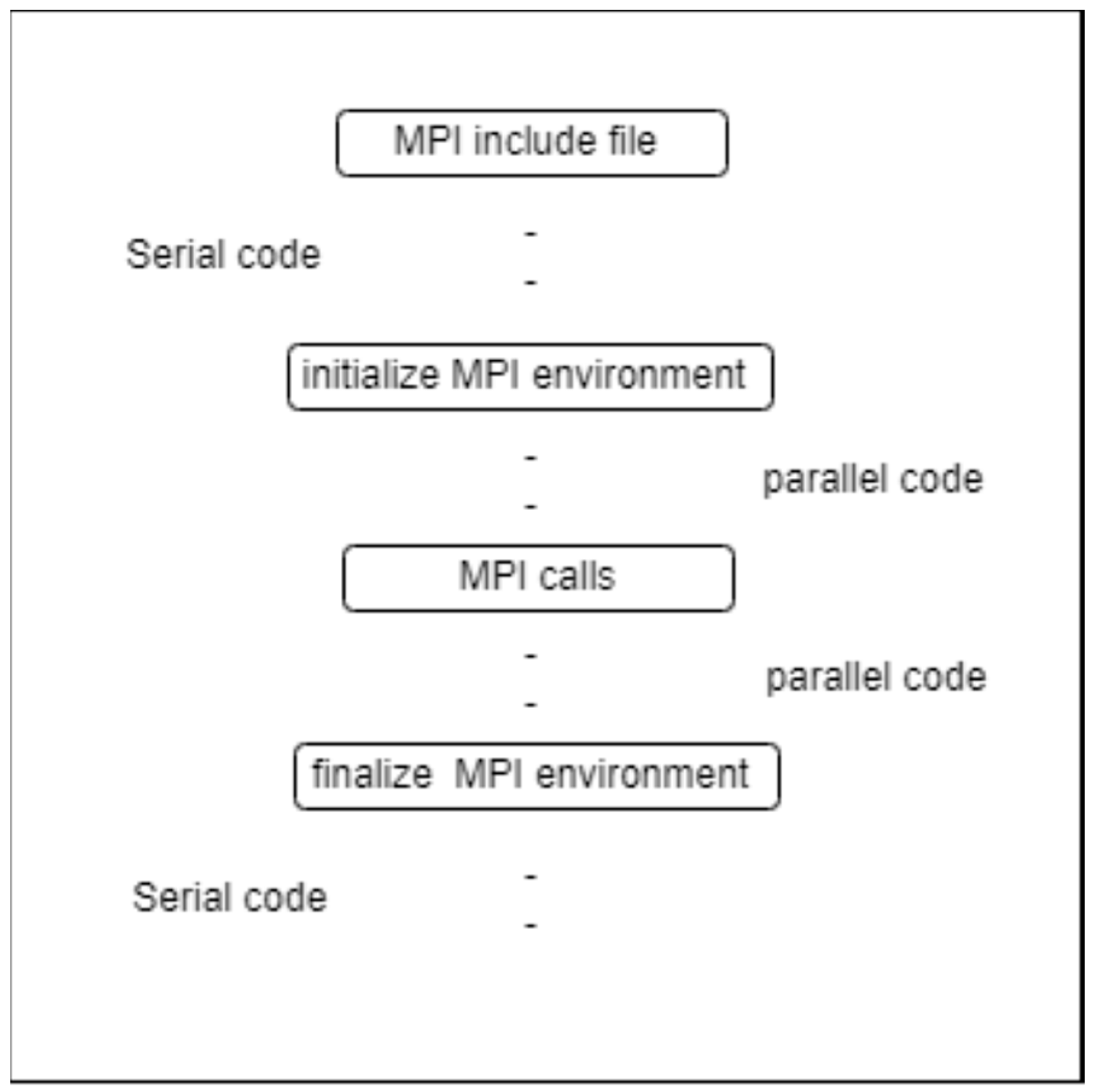
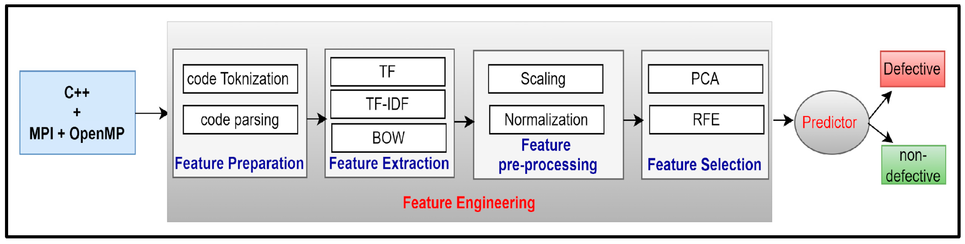
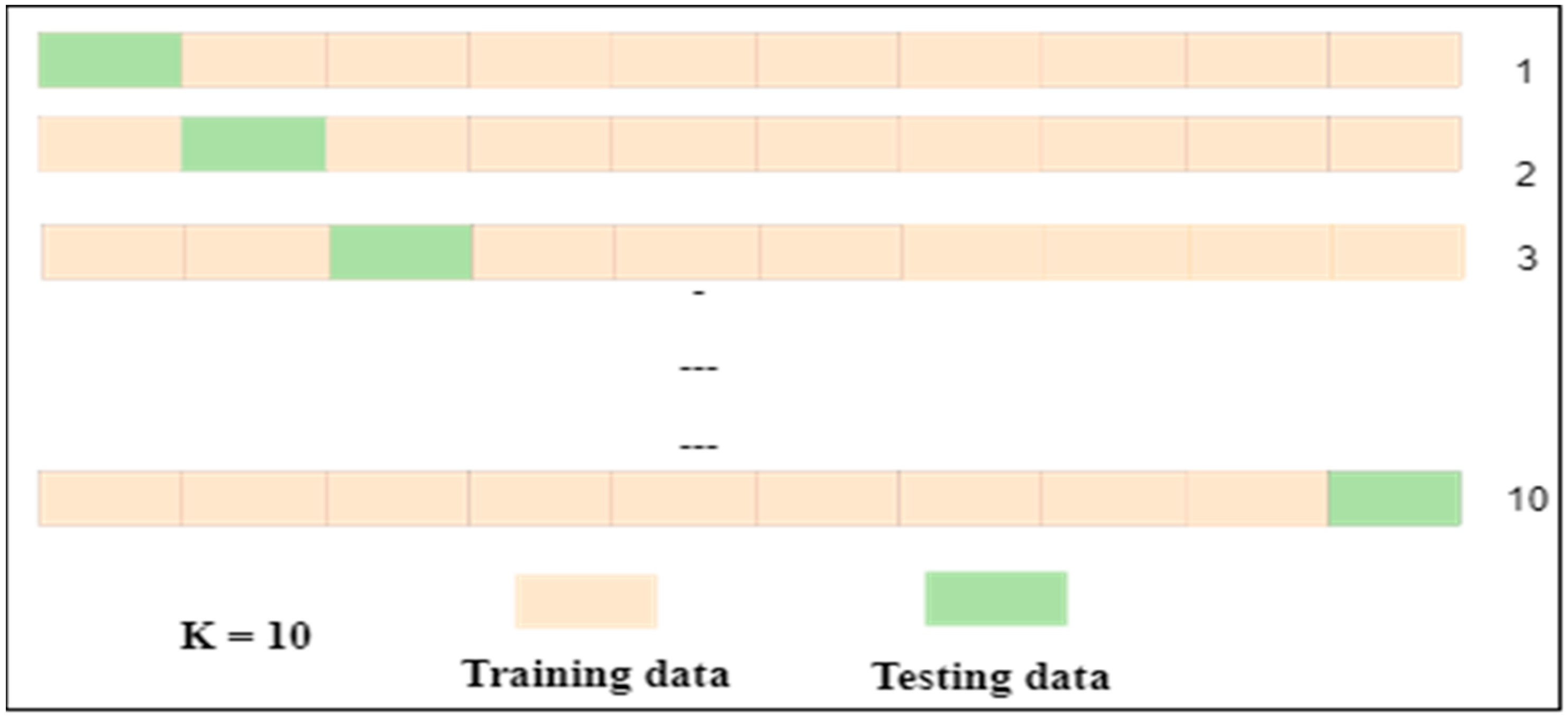
8. Conclusions

HPC systems promote hybrid programming implementation that integrates the MPI and OpenMP programming models. This integration can lead to more error-prone software, such as deadlock and race conditions. In this study, we proposed a machine learning model to predict defects in the source code of systems implemented in C++ with hybrid MPI and OpenMP program models. SDP used balanced datasets with hybrid MPI and OpenMP implemented in C++. The experimental results confirm that the trained model is efficient in classifying the source code file as defective or nondefective. The SVM classifier with TF and TF-IDF coupled with RFE achieved the highest performance (accuracy, F1 score, and AUC of 84%) when compared to other classifiers. NB, with different feature extraction techniques such as TF, TF-IDF, and Bow, achieved a high precision of 91% when applied with scaling and RFE techniques. In terms of recall, again, SVM achieved the highest percentage among the classifiers when it was applied with different methods and techniques, reaching up to 100%, with all defective codes correctly classified; this makes it an optimal classifier for predicting defective OpenMP and MPI code.

This research offers a promising solution to mitigate the increasing error rates in software development, thereby potentially reducing development costs and time while improving overall software quality and reliability. Our methodology reflects a thorough and well-rounded approach to the problem of defect prediction in hybrid model code. The integration of diverse feature extraction techniques, a range of classifiers, and comprehensive feature processing methods demonstrates the strength of our study, which lies in its methodological rigor and the breadth of techniques used. Our study is also valuable for future research as it serves as a foundation for developing and testing defect prediction models. Our research can also open new pathways for further studies, such as applying sophisticated ML techniques (such as deep learning) to predict other types of errors and defects or those written in other programming languages, and also exploring different feature extraction techniques (such as code embeddings), which could lead to more efficient prediction and thus promote error-free software.