Online Outdoor Terrain Classification Algorithm for Wheeled Mobile Robots Equipped with Inertial and Magnetic Sensors

Abstract

Terrain classification provides valuable information for both control and navigation algorithms of wheeled mobile robots. In this paper, a novel online outdoor terrain classification algorithm is proposed for wheeled mobile robots. The algorithm is based on only time-domain features with both low computational and low memory requirements, which are extracted from the inertial and magnetic sensor signals. Multilayer perceptron (MLP) neural networks are applied as classifiers. The algorithm is tested on a measurement database collected using a prototype measurement system for various outdoor terrain types. Different datasets were constructed based on various setups of processing window sizes, used sensor types, and robot speeds. To examine the possibilities of the three applied sensor types in the application, the features extracted from the measurement data of the different sensors were tested alone, in pairs and fused together. The algorithm is suitable to operate online on the embedded system of the mobile robot. The achieved results show that using the applied time-domain feature set the highest classification efficiencies on unknown data can be above 98%. It is also shown that the gyroscope provides higher classification rates than the widely used accelerometer. The magnetic sensor alone cannot be effectively used but fusing the data of this sensor with the data of the inertial sensors can improve the performance.

1. Introduction

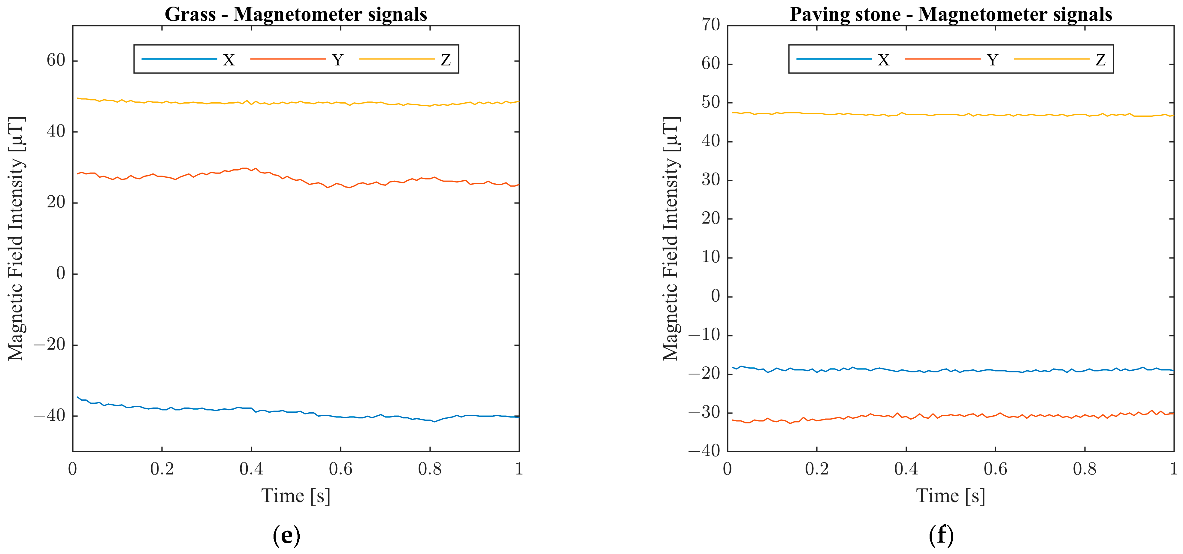
Terrain classification plays an important role in reliable mobile robot navigation problems [1,2], since the parasitic accelerations generated by different terrains inherently influence the state estimation performance as well as the path planner and control algorithms that rely on these results. As an example, a flat surface generates much less parasitic accelerations, thus the pose estimation is executed on reliable external acceleration integrations. On the other hand, bumpy terrains generate significant vibrations, which superimpose on the measurements of the accelerometer. In these cases, the separation of reference and observation vectors is difficult to execute reliably, thus the pose estimation becomes uncertain. The output of a terrain classification algorithm can help in characterizing the measurements with proper certainty measures, which contribute to both effective and reliable state estimation. This enables the establishment of algorithms that adaptively vary their parameters based on the identified environment of the robot.

Terrain classification systems apply onboard sensors. Various technologies were applied in relevant studies to identify the terrain type using mobile robots. Methods based on LiDAR [3] and camera [4,5,6,7,8] data are widely used, but these systems require embedded systems with high computational capacity, and they also have high costs. Beside the large amount of data which have to be processed, complex classification algorithms must be used, such as convolutional neural networks [8]. RGB-D [9] and sound-based [10,11] systems were also proposed by researchers.

Accelerometers, which measure linear acceleration in one or more axes, offer a low-cost alternative for terrain classification in the case of mobile robots, and were widely used in such applications [12,13,14,15,16,17,18,19,20,21,22].

The fusion of various technologies was also reported in relevant works, e.g., LiDAR and camera [23,24], sound and vibration [25], sound and camera [26,27,28], vibration and camera [29,30], camera, spectroscopy and nine degree-of-freedom (9DOF) inertial measurement unit (IMU) [31]. 9DOF IMUs consist of three tri-axial sensors, an accelerometer, a gyroscope, and a magnetometer.

Gyroscopes, which measure angular velocity around one or more axes, are widely used in pattern recognition applications, such as human movement or activity recognition [32,33]. In terrain classification tasks, these sensors were mainly tested together with accelerometers [31,34,35,36,37,38]. In a previous study, the authors of this paper showed that gyroscopes can provide significantly higher classification efficiencies than accelerometers using a frequency domain-based feature set [39].

Magnetometers are passive sensors that measure magnetic fields. Vector magnetometers measure the flux density value in a specific direction in three-dimensional space [40]. These devices are mainly used as compasses, since they can estimate the heading direction based on the Earth’s magnetic field. Magnetic sensors were also applied in pattern recognition-based applications, such as movement classification [32,33,41] and vehicle classification [42,43], which utilize the sensor measurements in a different way. In movement or activity classification systems, the methods utilize the changes in the orientation of the geomagnetic field vector compared to the sensor frame and are usually used together with inertial sensors. In vehicle detection/classification systems stationary sensors are applied and the distortions in the magnetic field are utilized, which are caused by metallic parts of the vehicles. Although, most outdoor mobile robots are equipped with magnetometers, due to their ability to serve as a compass, to the best knowledge of the authors, the raw measurements of these sensors were not utilized earlier in terrain classification methods.

Inertial sensor-based terrain classification methods most often rely on features extracted using the sensor signals, which are then forwarded to an appropriate classifier to determine the class. The base of the feature extraction is to extract information about the changes in the signals, which occur due to the movement of the sensors. Other solutions also exist, e.g., Reina et al. developed a model-based observer that estimates terrain parameters for vehicles based on two acceleration signals using a Kalman filter [12]. In [13], recurrent neural networks were applied using a three-axis sensor without extracting features on a dataset consisting of 14 terrain classes. In [34], acceleration, angular rate, and roll-pitch-yaw (RPY) data, which were provided by the 9DOF IMU sensor, were applied to form the feature vector. An ensemble classifier was applied to classify measurements into five classes: brick, concrete, grass, sand, and rock. In [31], angular acceleration, linear acceleration, and linear jerk were extracted using the signals of a 9DOF IMU. The IMU, the camera, and the spectroscopy-based classifiers were fused to classify terrains into 11 types.

Various feature extraction techniques were tested in related studies. Oliveira et al. utilized only the Z-axis of the accelerometer, which points to the ground, and the root mean square feature was used to classify 5 pavement types [14]. In [15], also only the Z-axis was used, and a Laplacian support vector machine (SVM) was applied with various time-domain features (TDFs) and frequency-domain features (FDFs) to classify six outdoor terrain types: natural grass, asphalt road, cobble path, artificial grass, sand beach, and plastic track. Weiss et al. applied signals of all three sensor axes and evaluated their applicability in the given task [16]. The components of the amplitude spectrum, which were computed using the fast Fourier transform (FFT), were utilized as features. An SVM-based classifier was applied in two experiments, i.e., a 3-class and a 7-class experiments. Magnitudes computed using the FFT from vibration signals were also the base of the method proposed in [17], where terrains were classified into clay, grass, sand, and gravel. In [18], 523 power spectrum density (PSD)-based features and 11 different statistical features were used to classify 4 indoor surface types. In [19], features were extracted in time, frequency, and time-frequency domains to classify the terrain into four types (hard ground, grass, small gravel, and large gravel). Bai et al. defined five outdoor terrain classes, concrete, grass, sand, gravel, and grass&stone, and applied spectral features from acceleration data to classify samples using artificial neural networks (ANN) [20]. In [21], Bai et al. proposed a deep neural network-based solution using a similar feature extraction concept. Mei et al. composed three feature sets using TDFs, FDFs, and PSD-based features, and made a comparative study using different classifiers to differentiate 8 outdoor terrain types: asphalt, cobble, concrete, artificial grass, natural grass, gravel, plastic, and tile [22]. DuPont et al. used magnitudes computed using the FFT for the acceleration in the Z-axis and the angular velocity around the X and Y axes [35]. The terrains were classified using probabilistic neural networks into six classes: asphalt, packed gravel, loose gravel, tall grass, sparse grass, and sand. In [36], more than 800 features were extracted from the inertial sensor signals for indoor terrain classification with a linear Bayes normal classifier. Hasan et al. applied altogether 60 different temporal, statistical and spectral features using accelerometer and gyroscope data together to classify 9 indoor surface types [37]. In [38], the components of the amplitude spectrum computed for the six channels of the IMU sensor were used together as inputs of the ANN to classify terrains into five classes, i.e., indoor floor, asphalt, grass, soil, and loose gravel.

This study deals with outdoor terrain classification using inertial and magnetic sensors in the case of wheeled mobile robots. The contributions of this work, which is the extension of an initial investigation presented by the authors in [44], can be summarized as follows:

• A novel online terrain classification algorithm is proposed, which applies only TDFs extracted from the raw accelerometer, gyroscope, and magnetometer signals. The chosen feature set has both low computational and low memory costs, which enables easy implementability. Classification is realized using multilayer perceptron (MLP) neural networks. The proposed algorithm is suitable to run online in real-time on the embedded system of the mobile robot or it can be used on a separate intelligent sensor that provides the classification results to the main control unit of the robot.
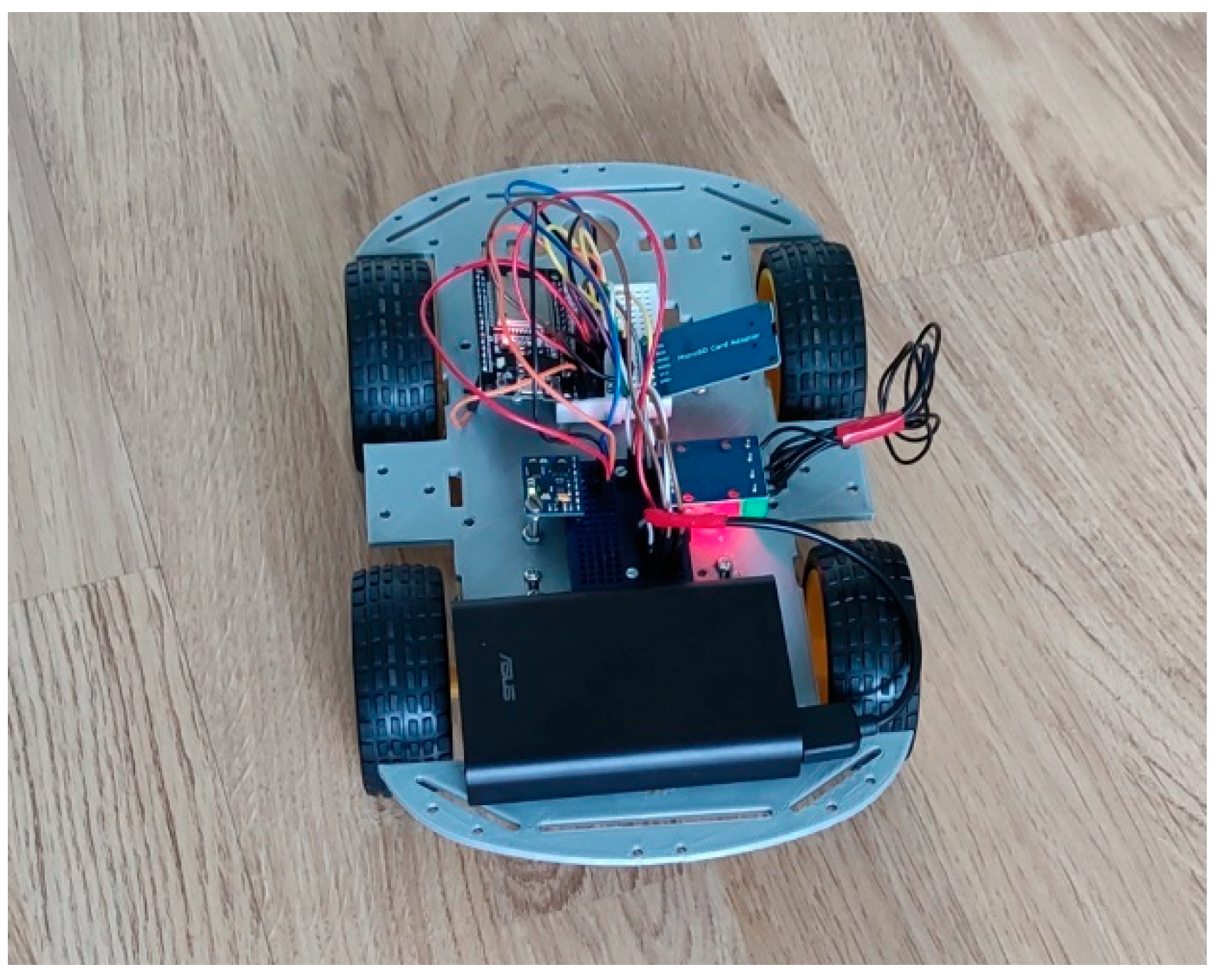
• The proposed algorithm is validated using a measurement database collected using a prototype measurement system. Tests are performed utilizing different processing window sizes and multiple robot speeds to examine their effect on recognition efficiency.
• Due to the previous considerations, it was reasonable to test the applicability of raw magnetometer data and the impact of the three sensor types in such an application. Thus, the features extracted using signals of the three sensor types are tested alone, in pairs, and together using the proposed algorithm.
• In the evaluation process, achieved results using different setups are compared with results obtained using a set of spectral features and with results obtained using the two feature sets together.

The rest of the paper is organized as follows. Section 2 presents the proposed terrain classification algorithm, while Section 3 describes the used measurement database. The experimental results achieved using different setups are discussed in Section 4, while Section 5 summarizes the results of the paper and gives potential future work directives.

2. Classification Algorithm

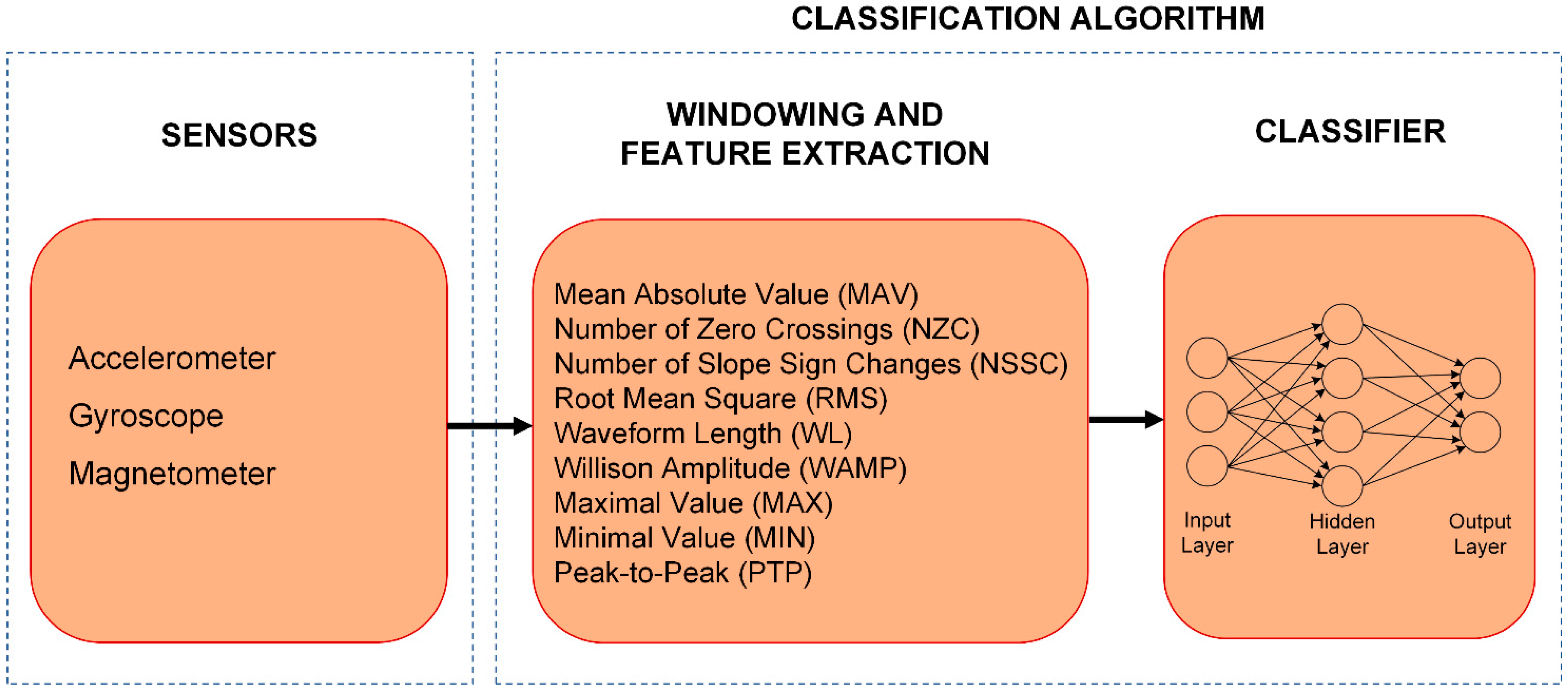
The proposed classification algorithm, which can be seen in Figure 1, consists of two main parts. In the first part, windowing and feature extraction are performed on raw sensor signals. The extracted features are then forwarded to the second part, where an MLP-based classifier is utilized to determine the class.

The classifier needs to be trained offline using training data, after which the trained MLP can be implemented and used online.

2.1. Windowing and Feature Extraction

Feature extraction is performed in fixed-size processing windows, which are shifted with also constant sizes. The shift size determines the overlap between windows and the frequency with which the algorithm updates the terrain class. It does not have any effect on the amount of data in the window.

One of the advantages of the applied features is that these do not require the transformation from time-domain to frequency-domain, which beside performing fast Fourier transform (FFT) requires the storage of the measurement values in the processing window.

Many popular TDFs require the storage of the measurement vector in the processing window, and can be calculated only before the classification process. e.g., in the case of features such as standard deviation, skewness, and kurtosis, the mean value must be subtracted from each of the measurement values in the processing window. The mean value can only be computed at the end of the processing window, so all measurements in the window must be stored. In the proposed algorithm, all selected feature types can be updated after every measurement, and they do not need the storage of the measurement vector in the processing window. At most two previous measurement values are required to update the features. This enables easier implementation, and real-time online operation on the embedded system of the robot.

The selected TDFs are discussed as follows:

• Mean absolute value (MAV):

$$\mathrm{MAV}=\frac{1}{N}{{\displaystyle \sum }}_{i=1}^N\left|x_i\right|,$$

(1)

where $x_i$ is the ith measurement value, and N is the number measurements in the processing window.

• Number of zero crossings (NZC):

$$\mathrm{NZC}={{\displaystyle \sum }}_{i=1}^{N-1}\left[\mathrm{sgn}\left(x_i·x_{i+1}\right){{\displaystyle \cap }}^{}\left|x_i-x_{i+1}\right|\ge th\right],\mathrm{sgn}\left(x\right)=\{\begin{array}{l}1, \mathrm{if}\left(x\ge 0\right)\\ 0, \mathrm{o}\mathrm{t}\mathrm{h}\mathrm{e}\mathrm{r}\mathrm{w}\mathrm{i}\mathrm{s}\mathrm{e}\end{array},$$

(2)

where th is the threshold, which is defined using the peak-to-peak noise level.

• Number of slope sign changes (NSSC):

$$\mathrm{NSSC}={{\displaystyle \sum }}_{i=2}^{N-1}\left[f\left[\left(x_i-x_{i-1}\right)·\left(x_i-x_{i+1}\right)\right]\right],f\left(x\right)=\{\begin{array}{l}1, \mathrm{if}\left(x\ge th\right)\\ 0, \mathrm{o}\mathrm{t}\mathrm{h}\mathrm{e}\mathrm{r}\mathrm{w}\mathrm{i}\mathrm{s}\mathrm{e}\end{array},$$

(3)

• Root mean square (RMS):

$$\mathrm{RMS}=\sqrt{\frac{1}{N}{{\displaystyle \sum }}_{i=1}^N{x}_i^2},$$

(4)

• Waveform length (WL):

$$\mathrm{WL}={{\displaystyle \sum }}_{i=1}^{N-1}\left|x_{i+1}-x_i\right|,$$

(5)

• Willison amplitude (WAMP):

$$\mathrm{WAMP}={{\displaystyle \sum }}_{i=1}^{N-1}\left[f\left(x_i-x_{i+1}\right)\right],f\left(x\right)=\{\begin{array}{l}1, \mathrm{if}\left(x\ge th\right)\\ 0,\mathrm{o}\mathrm{t}\mathrm{h}\mathrm{e}\mathrm{r}\mathrm{w}\mathrm{i}\mathrm{s}\mathrm{e}\end{array},$$

(6)

• Maximal value (MAX):

$$\mathrm{MAX}=\max \left(x_i\right),$$

(7)

• Minimal value (MIN):

$$\mathrm{MIN}=\min \left(x_i\right),$$

(8)

• Peak-to-peak (PTP):

$$\mathrm{PTP}=\mathrm{MAX}-\mathrm{MIN}.$$

(9)

Some features were not applied for all three sensor types. Raw accelerometer measurements suffer from the gravitational acceleration, which can be neglected using complex pose estimation methods, which require additional computation. Due to this effect, the MAV, RMS, MAX, and MIN features would largely differ if the robot would move parallel with the Earth’s surface or uphill. Based on the previous considerations, these features were not utilized in the case of the accelerometer. In the case of the magnetometer, the changes in the orientation of the magnetic field vector are utilized in the classification process. Since the components of the vector act as an unknown bias in the measurements, the same features, i.e., the MAV, RMS, MAX, and MIN, were also not utilized with this sensor type.

2.2. Classifier

A three-layer Multi-Layer Perceptron (MLP) neural network was chosen as the classifier in the proposed algorithm, since it proved to be an optimal solution for similar online pattern recognition tasks based on classification efficiency and implementability [32].

MLPs are feedforward neural networks, where neurons are organized into an input, an output, and one or more hidden layers. All layers are fully connected to the following one through weighted connections. A neuron has an activation function that maps the sum of its weighted inputs to the output. These ANNs are usually trained using the backpropagation algorithm.

In the proposed algorithm, a three-layer neural network is used with one hidden layer. A feature vector is composed of the TDFs computed in the feature extraction stage of the algorithm. The feature values are computed separately for the three axes of the applied different sensor types. In setups utilizing multiple sensors, the data of the different sensors are fused by using the extracted features together in the feature vector. The computed feature vector forms the input of the MLP, thus, the number of inputs is equal to the number features in the given setup. In the output layer a neuron is assigned to each class. In the hidden layer, the hyperbolic tangent sigmoid activation function is applied, while the linear transfer function is utilized in the output layer. The neuron with the highest output value in the output layer is declared as the class for the given input vector. The optimal number of neurons in the hidden layer must be found by testing different configurations.

3. Applied Measurement Data

3.1. Prototype Measurement System

To obtain measurement data on which the proposed terrain classification algorithm can be tested, a mobile robot was constructed with appropriate sensors. The constructed wheeled mobile robot can be seen in Figure 2. The size of the robot was 158 × 255 × 45 mm, while its mass was 0.595 kg. The robot had two driven and two additional wheels. The wheelbase was 116 mm, the track width was 132 mm, and the wheel radius was 65 mm.

A 9DOF sensor board was also installed on the constructed robot, which consists of a tri-axial magnetometer, a tri-axial accelerometer, and a tri-axial gyroscope. The main characteristics of the sensors can be seen in

Table 1. Main characteristics of the applied sensors.

Characteristic	Accelerometer	Gyroscope	Magnetometer
type	ADXL345	ITG3200	HMC5883L
technology	microelectromechanical system (MEMS)	MEMS	anisotropic magnetoresistive (AMR)
measurement range	±16 g	±2000 deg/s	±810 µT
resolution	13-bit	16-bit	12-bit
highest sampling frequency	3.2 kHz	8 kHz	160 Hz

.

A microcontroller-based ESP32 unit, which was manufactured by Espressif Systems, Shanghai, China, was used for motor control via H-bridges, which vary the speed of the motors based on the pulse width modulation (PWM) duty cycle. The ESP32 was also responsible for reading measurements from the inertial sensors and storing the data.

3.2. Data Acquisition

Measurement data acquisition was done for six different outdoor terrain types, which can be seen in Figure 3. These terrain classes are the following:

• Concrete
• Grass
• Pebbles
• Sand
• Paving stone
• Synthetic running track

Measurements were collected in sessions, which were 4.5 s long, and the applied sampling rate was 400 Hz for both inertial sensors and 100 Hz in the case of the magnetometer. For all six classes data were recorded in seven sessions, which resulted in 31.5 s measurement data for each terrain type. The seven sessions within a class were chosen to be at different locations with as most diverse terrains as possible. All measurements were performed with two different motor speeds, which were set using the PWM, to explore its effect on the algorithm. The PWM duty cycles were constant during the measurements since the goal of the algorithm is to provide information to a sensor fusion framework, which can estimate the true speed of the mobile robot. The speed was not measured during data acquisition, and it was probably varying due to slips of the mobile robot. The algorithm should provide reliable data without knowledge of the PWM duty cycle or the encoder measurements, it only relies on raw inertial and magnetic sensor data. The two used PWM duty cycles were 86% and 100%.

Figure 4 shows parts of the signals for the three sensor types from the measurement data collected for two classes, i.e., grass and paving stone.

4. Experimental Results

4.1. Datasets and Test Setups

Altogether 63 different datasets were tested and evaluated with the proposed algorithm based on different setups.

Three processing window sizes were tested: 0.32 s, 0.64 s, and 1.28 s. The applied window shift size was 0.05 s for all three segment sizes. The reason for setting a small shift size was to generate as many training samples as possible from the available data. The applied shift size in a real application should be set based on the requirements.

Different datasets were constructed based on the used sensor configurations. The three sensor types were tested alone, in pairs, and together, to examine their possibilities in the application. The applied feature types were extracted for all sensor axes separately.

To explore the effect of different speeds on the proposed algorithm, the measurement data using the applied two speeds were tested separately and together.

In the case of all setups, the training datasets were formed using measurements from four of seven sessions, while the remaining three sessions formed the validation datasets. Validation datasets were not applied during the training of the MLPs and were used as unknown inputs to test the performance of the trained classifiers.

The hyperparameters of the MLP training process can be found in

Table 2. Hyperparameters of the MLP training process.

Hyperparameter	Value
training function	scaled conjugate gradient backpropagation
performance function	mean squared error (MSE)
maximum number of epochs to train	4000
performance goal	0
maximum validation failures	20
minimum performance gradient	10−7
maximum time to train in seconds	inf

. During the training of the MLPs, 70% of the training data were used as training inputs, and the remaining 30% as validation inputs. The training was tested with 1–40 hidden layer neurons for all setups, and all configurations were tested 4 times, since the achievable performance of the ANNs largely depends on the initial random weights. During performance evaluation, the results of the configuration which achieved the highest recognition efficiencies on validation data were used. The tested neuron numbers in the hidden layer proved to be sufficient, since convergence could be noticed in the recognition rate on unknown samples for all setups.

Classification efficiencies (E) were used as the performance metric, which can be calculated using the following equation:

$$E(\%)=\frac{N_C}{N_S}·100,$$

(10)

where N_C is the number of correctly classified samples and N_S is the number of all samples.

In the evaluation process, achieved results using the TDFs were compared with recognition efficiencies provided by FDFs for all setups. The applied spectral feature set was the same as in [39], which consists of the following features: spectral energy, median frequency, mean frequency, mean power, peak magnitude, peak frequency, and variance of the central frequency. To explore if the FDFs carry any further information compared to the proposed time domain-based feature set, the two feature sets were also tested together.

4.2. Performance Evaluation

The achieved highest classification efficiencies on training and validation data using the proposed algorithm can be seen in

Table 3. Achieved classification efficiencies (%) on training and validation data based on different sensor and speed combinations for the three processing window sizes.

Sensor	Speed	Processing Window Size and Data Type
		0.32 s		0.64 s		1.28 s
		Training	Validation	Training	Validation	Training	Validation
Accelerometer	L	89.26	81.59	94.81	87.66	100.00	92.45
	H	94.43	82.26	99.51	86.72	99.94	91.49
	L and H	86.44	76.51	95.13	82.14	98.96	90.41
Gyroscope	L	97.99	94.24	99.62	96.25	100.00	99.22
	H	96.59	87.55	99.51	91.63	100.00	97.66
	L and H	94.60	90.16	97.40	94.99	100.00	97.05
Magnetometer	L	66.87	53.95	75.92	60.02	88.02	66.58
	H	58.94	58.90	75.54	63.28	75.13	63.72
	L and H	59.24	55.02	68.91	59.09	84.41	62.85
Accelerometer, gyroscope	L	99.30	94.18	99.89	96.32	100.00	99.83
	H	99.35	91.43	100.00	92.71	100.00	96.70
	L and H	97.42	91.73	100.00	95.85	100.00	98.18
Accelerometer, magnetometer	L	93.17	86.01	97.08	91.49	99.87	94.79
	H	97.14	86.08	99.89	89.11	100.00	93.58
	L and H	91.27	80.42	98.38	85.46	100.00	90.80
Gyroscope, magnetometer	L	97.79	93.91	100.00	97.62	100.00	99.74
	H	98.24	92.30	100.00	96.18	100.00	98.52
	L and H	96.34	92.24	100.00	96.28	100.00	98.87
Accelerometer, gyroscope, magnetometer	L	98.59	92.64	100.00	98.05	100.00	99.65
	H	98.85	92.70	100.00	95.96	100.00	97.31
	L and H	98.27	91.03	100.00	96.43	100.00	97.79

. The results are given based on different used sensor and speed combinations for the three processing window sizes. The used abbreviations are the following: L—lower speed, H—higher speed.

Analyzing the achieved classification efficiencies with the proposed TDF-based algorithm using different processing window widths, it can be seen that the recognition rate on both training and unknown data rises by increasing the size of the segment. On validation data, above 94% efficiency can be achieved even using the smallest window size, which is 0.32 s. The highest classification efficiencies for the two larger segment sizes were above 98%. In the case of training data, the classification efficiencies were above 95% for most of the setups even with the smallest window size, thus, the increases were smaller. The largest effect of the increase in the processing window size can be noticed for the setups where the accelerometer and the magnetometer data were utilized alone. In the case of the accelerometer, the increase was around 5% for both jumps in the segment size. Using the data of the magnetic sensor even above 10% increases were noticed, especially in the case of the training data.

Based on the obtained results using different robot speeds, difference can be noticed in some setups between the lower and the higher speed. The gyroscope results in higher recognition rates with the lower speed on unknown data, where the difference can be above 5% with the two smaller segment sizes. This can be noticed also in the setups where the gyroscope data were fused with other sensors, but with smaller differences. By combining the two speeds in the datasets, in most setups the classification efficiency decreases compared to the results achieved using single speeds. For other datasets the recognition rates are between the results obtained using the two speeds separately. It can be noticed that the use of multiple speeds together has a larger effect on setups where accelerometer data is applied, since in these cases the decrease in efficiency is larger.

The results based on different sensor combinations where the two speeds were used together show that the highest recognition rates were achieved using the setups where the gyroscope data were present. The highest obtained classification efficiencies were above 91%, 96% and 98% for the three tested segment sizes, respectively. Utilizing data of only a single sensor type, significantly higher results were obtained using gyroscope data than with accelerometer data, which is widely used in terrain classification applications. The difference can be even more than 10% depending on the window size. Using the smallest window size, the accelerometer and the gyroscope-based results were 76.51% and 90.16%, respectively. With the largest segment size, the recognition rates increase to 90.41% and 97.05%, respectively. The magnetometer data alone cannot provide acceptable classification efficiencies, since even with the largest processing window size the results were 62.85%. Fusing the data of this sensor with the inertial sensors can improve the recognition rates, especially in the case of smaller window sizes. e.g., using the accelerometer and the magnetic sensor data together 80.42% was obtained, which was almost a 4% improvement compared to the accelerometer-based result.

Table 4. Misclassification rates (%) on validation data when the data of the three sensors for both speeds were utilized together and the features were extracted in the smallest processing window.

		Output Class						Sum
		1	2	3	4	5	6
Target class	1			3.41		7.23		10.64
	2			3.82	16.47		1.20	21.49
	3		3.61				0.20	3.81
	4		2.61					2.61
	5	7.63		1.61			3.41	12.65
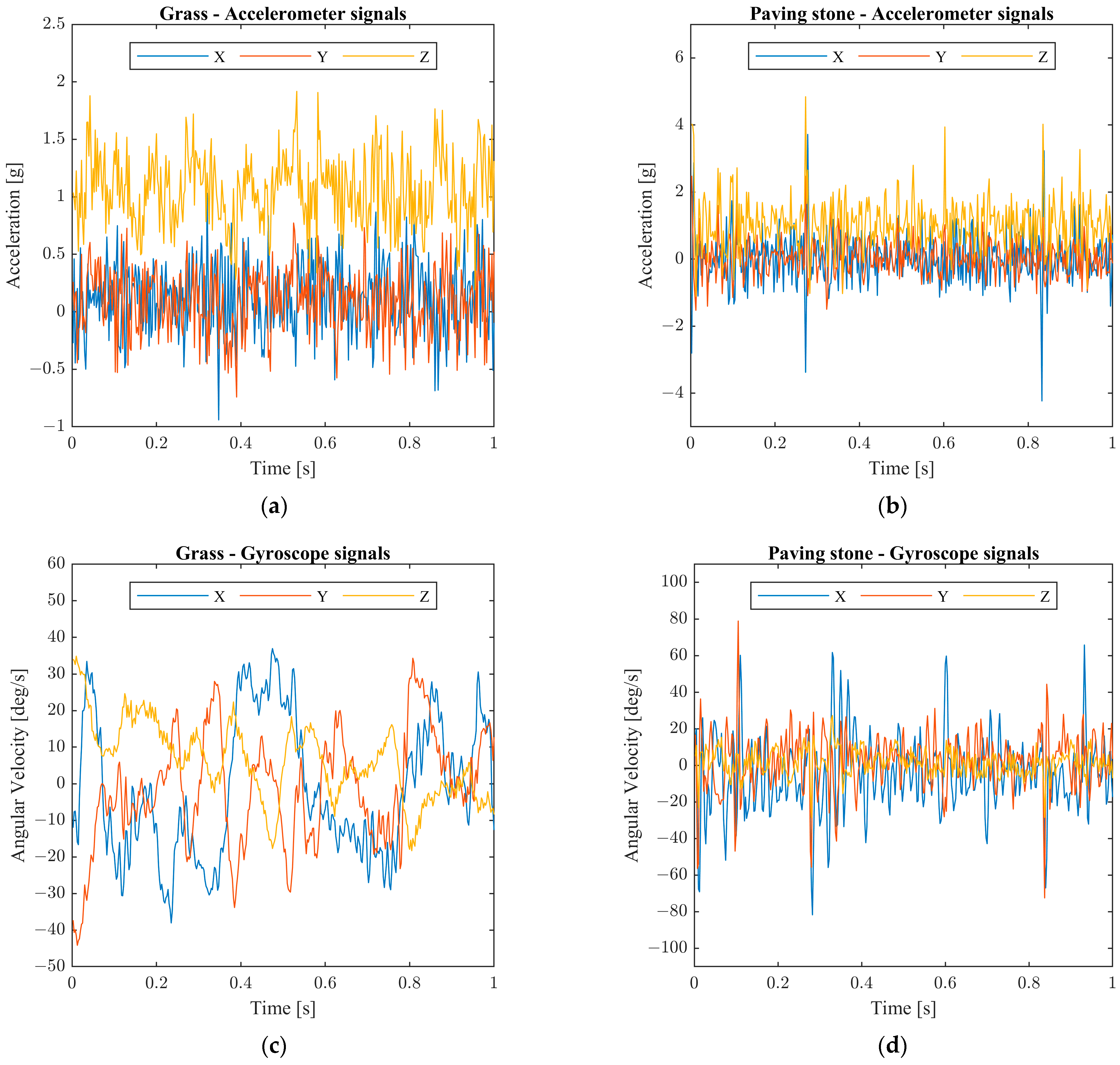
	6	1.41		0.20		1.00		2.61

presents the misclassification rates on validation data when the data of the three sensors for both speeds were utilized together and the features were extracted in the smallest processing window. The overall classification efficiency for this setup was 91.03%. It can be observed from the results that above 10% miss rate can be noticed for three classes, i.e., concrete, grass, and paving stone. Grass was recognized with the lowest efficiency since the misclassification rate for this class was 21.49%. Within this class 16.47% of the samples were classified as sand. Higher, above 7%, misclassification rates can be noticed between concrete and paving stone.

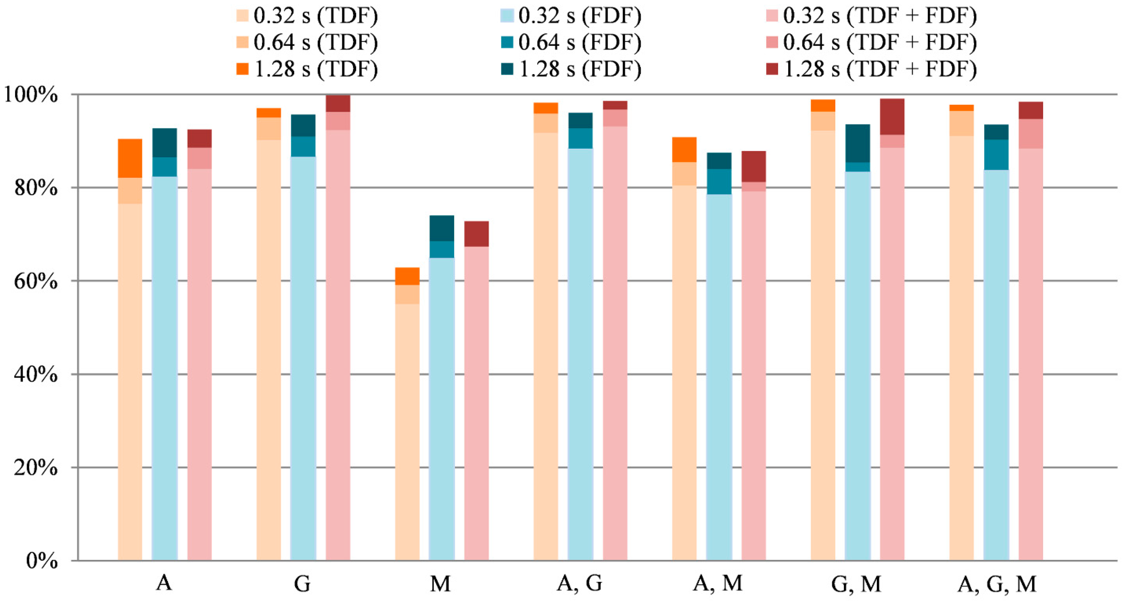
To explore the performance of the proposed TDF-based feature set, the results were compared with results obtained using an FDF-based feature set [39] and the two feature sets together. The obtained classification efficiencies on validation data using the different feature extraction techniques are summarized in Figure 5. Recognition rates are given based on different sensor combinations using data collected for both speeds together. The used abbreviations are the following: A—accelerometer, G—gyroscope, M—magnetometer.

It can be observed from the obtained results that the proposed feature set outperforms the FDF-based feature set in most setups, except where accelerometer and magnetometer data were utilized alone. Significant, more than 10%, difference can be only noticed using the magnetometer data, where almost 75% efficiency can be obtained using the FDFs. In case of the accelerometer, the differences are smaller, around 2–3%. In other setups, the proposed TDF set provides mostly 3–5% better performance compared to the FDF-based set, but it can reach even above 10% for some datasets. Using the two feature sets together, but not considering the setups where the FDFs provide higher efficiencies than the TDFs, can increase the classification efficiencies. The difference is not significant, mainly 1–2%, which shows that the FDF does not carry much further information compared to the information extracted using the proposed feature set.

It is also very important to explore the performance that can be achieved when the classifiers are trained and tested using measurements recorded with different speeds. To evaluate the results in this perspective, the trained MLPs using the L speed measurements were tested with the features extracted using the H speed measurements, and vice versa.

Table 5. Achieved classification efficiencies (%) on training and test data using the 0.32 s processing window size when the MLPs were trained and tested using measurement recorded with different speeds.

Sensor	Used Speed Data for Training and Validation	Used Speed Data for Testing	TDF		FDF
			Validation	Test	Validation	Test
Accelerometer	L	H	81.59	56.00	84.61	65.00
	H	L	82.26	53.61	88.15	63.02
Gyroscope	L	H	94.24	73.26	90.96	76.85
	H	L	87.55	75.42	86.21	72.63
Magnetometer	L	H	53.95	47.73	85.54	21.00
	H	L	58.90	41.25	71.62	16.50
Accelerometer, gyroscope	L	H	94.18	74.30	91.90	74.27
	H	L	91.43	73.58	89.83	73.95
Accelerometer, magnetometer	L	H	86.01	62.28	91.10	44.23
	H	L	86.08	58.49	82.33	43.72
Gyroscope, magnetometer	L	H	93.91	68.42	90.70	50.43
	H	L	92.30	71.00	84.34	61.65
Accelerometer, gyroscope, magnetometer	L	H	92.64	77.42	94.11	45.12
	H	L	92.70	72.09	86.21	64.57

,

Table 6. Achieved classification efficiencies (%) on training and test data using the 0.64 s processing window size when the MLPs were trained and tested using measurement recorded with different speeds.

Sensor	Used Speed Data for Training and Validation	Used Speed Data for Testing	TDF		FDF
			Validation	Test	Validation	Test
Accelerometer	L	H	87.66	63.88	89.61	65.62
	H	L	86.72	57.05	90.77	62.93
Gyroscope	L	H	96.25	69.88	94.16	78.70
	H	L	91.63	70.63	91.99	76.72
Magnetometer	L	H	60.02	51.39	82.40	24.00
	H	L	63.28	42.58	76.98	20.66
Accelerometer, gyroscope	L	H	96.32	77.06	96.75	74.21
	H	L	92.71	77.55	93.72	75.97
Accelerometer, magnetometer	L	H	91.49	66.45	92.79	43.51
	H	L	89.11	50.16	83.91	41.28
Gyroscope, magnetometer	L	H	97.62	71.09	98.34	49.54
	H	L	96.18	73.75	86.44	51.52
Accelerometer, gyroscope, magnetometer	L	H	98.05	80.09	97.84	53.46
	H	L	95.96	69.88	86.58	64.35

and

Table 7. Achieved classification efficiencies (%) on training and test data using the 1.28 s processing window size when the MLPs were trained and tested using measurement recorded with different speeds.

Sensor	Used Speed Data for Training and Validation	Used Speed Data for Testing	TDF		FDF
			Validation	Test	Training	Validation
Accelerometer	L	H	92.45	66.07	92.97	63.65
	H	L	91.49	53.35	94.79	66.67
Gyroscope	L	H	99.22	78.57	98.61	79.02
	H	L	97.66	64.36	96.35	76.30
Magnetometer	L	H	66.58	50.41	79.25	25.93
	H	L	63.72	47.47	77.95	18.71
Accelerometer, gyroscope	L	H	99.83	80.17	98.87	77.72
	H	L	96.70	74.37	96.53	78.94
Accelerometer, magnetometer	L	H	94.79	65.37	97.05	42.45
	H	L	93.58	63.73	92.27	47.92
Gyroscope, magnetometer	L	H	99.74	66.22	99.74	54.43
	H	L	98.52	74.89	89.67	68.82
Accelerometer, gyroscope, magnetometer	L	H	99.65	74.55	99.83	53.61
	H	L	97.31	64.51	98.18	75.41

show the obtained results for the three tested processing window sizes, i.e., 0.32 s, 0.64 s, and 1.28 s, respectively. The classification efficiencies in the tables are given for validation and test data. Validation datasets were formed from data not used during training, but from the sessions of the same speed as used for training, while test datasets were formed using data of the other speed. The FDF-based results are also included in the tables for comparison. It can be observed from the obtained results that such classifiers must be trained using a wide range of speeds since the classification efficiencies significantly decrease by using different speeds for training and testing. Comparing different sensor combinations, the gyroscope data showed to be more universal for different speeds than the accelerometer data. The magnetometer data-based recognition rates drastically decrease when the speed is different, especially with FDFs, where the classification efficiencies were below 30%. It can be also noticed from the results that the proposed TDF-based feature set provides significantly better results than the FDF-based when data of multiple sensors are used together.

4.3. Implementation

The implementation of the proposed method requires multiple steps. Different classifiers should be developed for different types of mobile robots since many features of the mobile robot (such as size, mass, wheelbase, track width, etc.) affect the classification algorithm. The first step is to collect a measurement database for the defined terrain classes using the applied robot in a wide range of speeds. The feature extraction and the training of the MLP classifiers must be performed offline. Many options must be considered to find the optimal setup. Both the required memory for the implementation and the processing time of the MLP depend on the number of inputs and the number of hidden layer neurons so it is important to minimize both besides maximizing the classification efficiency [32]. The number of inputs is defined by the number of used features, which depend on the number of used sensors. Based on the achieved results in this study, it is reasonable to test various sensor combinations with the required processing window size. The optimal MLP that should be implemented on the embedded system should be chosen based on the hardware limitations defined by the used embedded system and the achievable classification efficiencies of different setups. The size of the window shift, which defines the period with which the algorithm updates the terrain class, should be chosen based on the requirements of the application in which the method is used.

The proposed method uses the highest output value of the MLP as the predicted class. This assumes that all possible terrain types are known in advance. This can lead to uncertain predictions in applications where the mobile robot can encounter unknown terrain types. To handle these situations, possible solutions can be to add an “unknown” class to the outputs of the MLP or to use a probability threshold to reject such uncertain predictions.

5. Conclusions

In this paper, a novel terrain classification algorithm was proposed, which can run on the embedded system of a mobile robot with low requirements in both memory and computation. The algorithm applies only time-domain analysis in the feature extraction process and the MLP is used as classifier.

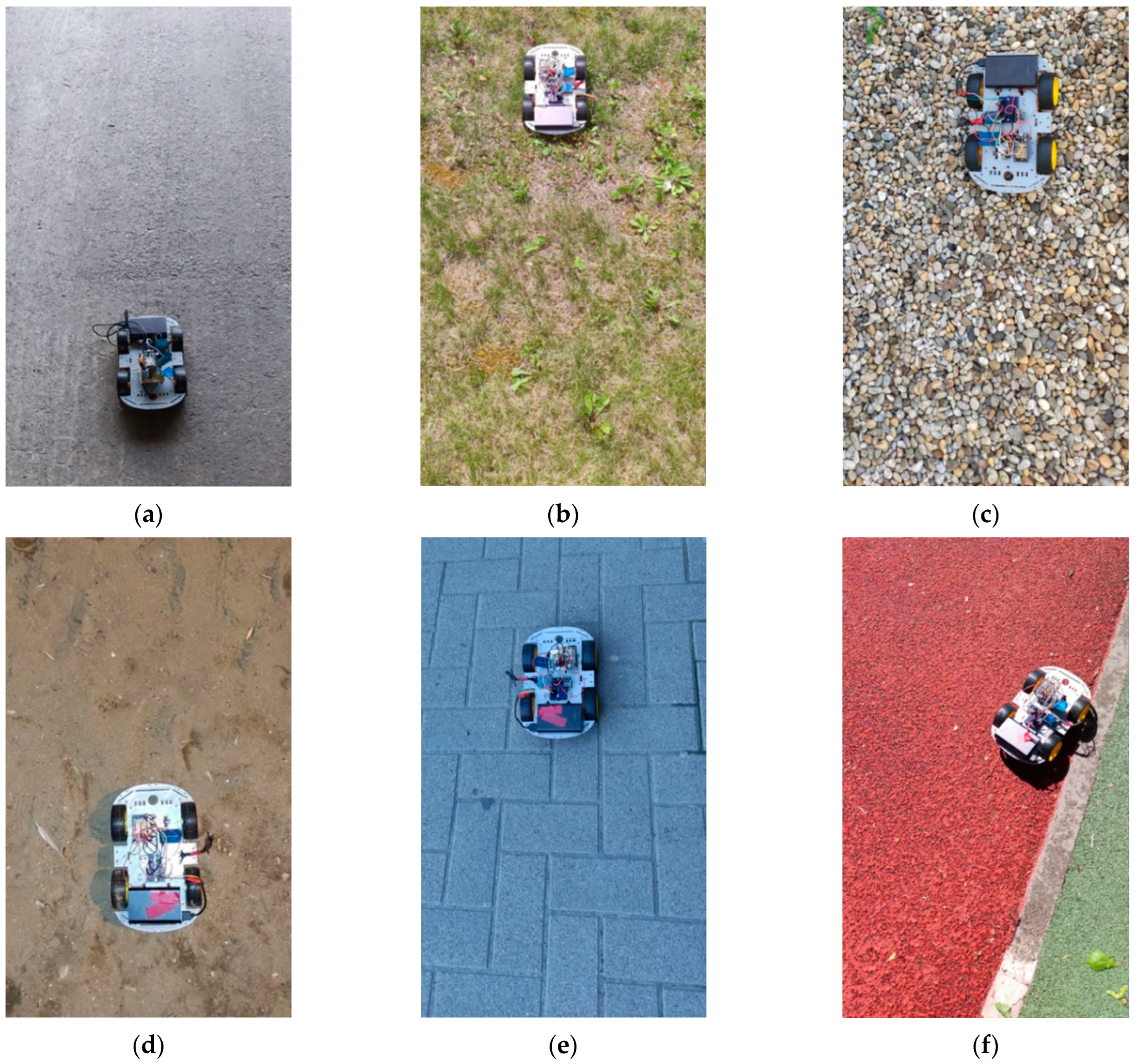
The algorithm was tested using measurements collected for six different outdoor terrain types with a prototype measurement system. Various setups were tested based on used sensor data, different processing window sizes, and robot speeds. The achieved results were compared with results obtained using a previously proposed feature set, which consists of only FDFs, and the two feature sets together.

The achieved classification efficiencies show significant results, since above 98% can be reached in some setups. It was also shown that the gyroscope is well usable in terrain classification systems and provides much higher recognition rates than the accelerometer. The magnetometer data alone cannot be effectively used in the given application, but it can improve the performance of the inertial sensors. The proposed algorithm also outperforms the FDF-based algorithm in most setups.

The main goal in the future is to implement the proposed terrain classification method into a novel sensor fusion framework, which can utilize the provided information to improve the pose estimation of the mobile robot. Other future plans include testing the algorithm on measurements recorded in a wider range of speeds for various motion types, such as cornering. Selecting the features with the highest effect on recognition accuracy using an appropriate feature selection method would be also reasonable, because this would further decrease the required computation. A pose estimator could be also implemented to neglect the effect of gravitational acceleration, since this could enable the usage of further features in the case of the accelerometer.