
Speech Emotion Recognition Based on Deep Residual Shrinkage Network

 , , ,
, , ,
Abstract
1. Introduction
2. Related Work
3. Materials and Methods
3.1. Mel-Spectrogram of Speech
3.2. Deep Residual Shrinkage Network
3.2.1. Residual Shrinkage Building Unit
- (1)
- Take absolute values for all input features;
- (2)
- An feature A is obtained after global average pooling (GAP);
- (3)
- Input A into a fully connected network. The sigmoid function is on the last layer, and the output is a coefficient in the range of 0 to 1;
- (4)
- is the threshold to be learned.
3.2.2. Soft Thresholding
3.2.3. Self-Attention Mechanism
3.3. Bi-Directional Gated Recurrent Unit
- (1)
- Reset gate and update gate
- (2)
- Hidden status
- (3)
- Bi-directional gated recurrent unit
4. Results
4.1. Datasets Introduction
4.2. Activation Funtion
4.3. Optimization of RSBU Quantity
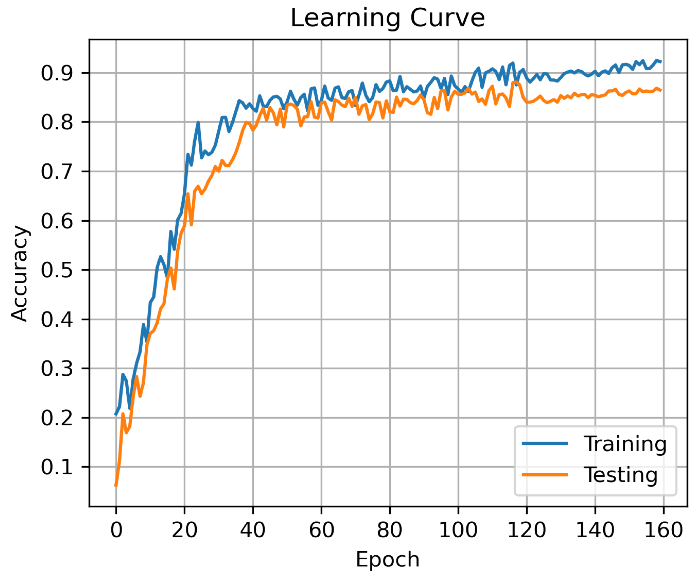
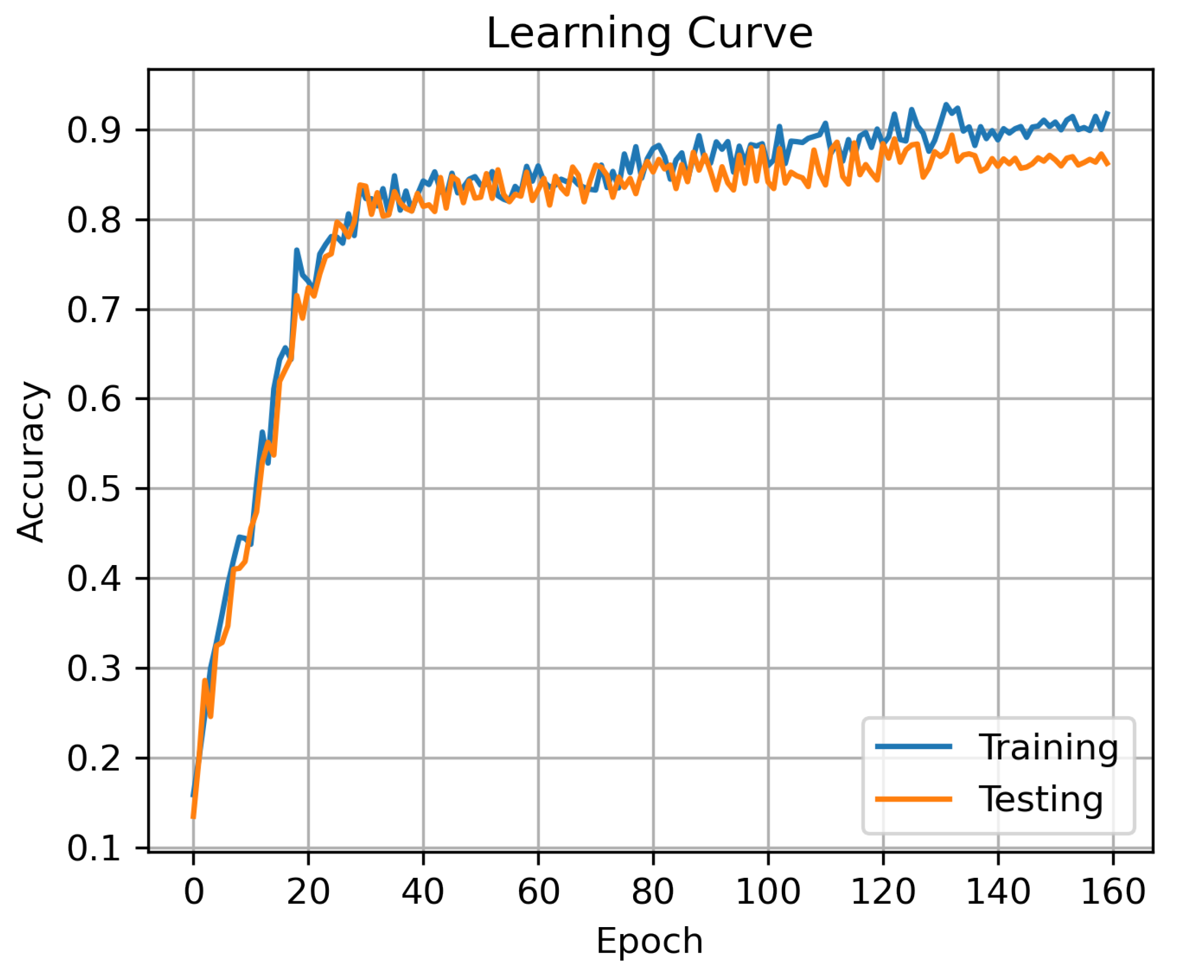
4.4. Performance of DBSN-BiGRU
5. Discussion
5.1. Results Discussion
5.2. Result Comparison and Discussion
5.3. Complexity Analysis and Discussion
5.4. Real-Life Applications Discussion
6. Conclusions
Author Contributions
Funding
Institutional Review Board Statement
Informed Consent Statement
Data Availability Statement
Acknowledgments
Conflicts of Interest
References
- Wani, T.M.; Gunawan, T.S.; Qadri SA, A.; Kartiwi, M.; Ambikairajah, E. A comprehensive review of speech emotion recognition systems. IEEE Access 2021, 9, 47795–47814. [Google Scholar] [CrossRef]
- Akçay, M.B.; Oğuz, K. Speech emotion recognition: Emotional models, databases, features, preprocessing methods, supporting modalities, and classifiers. Speech Commun. 2020, 116, 56–76. [Google Scholar] [CrossRef]
- Zvarevashe, K.; Olugbara, O. Ensemble learning of hybrid acoustic features for speech emotion recognition. Inf. Process. Manag. 2020, 13, 70. [Google Scholar] [CrossRef]
- Zhao, Z.; Bao, Z.; Zhao, Y.; Zhang, Z.; Cummins, N.; Ren, Z.; Schuller, B. Exploring deep spectrum representations via attention-based recurrent and convolutional neural networks for speech emotion recognition. IEEE Access 2019, 7, 97515–97525. [Google Scholar] [CrossRef]
- Bhavan, A.; Chauhan, P.; Shah, R.R. Bagged support vector machines for emotion recognition from speech. Knowl.-Based Syst. 2019, 184, 104886. [Google Scholar] [CrossRef]
- Fahad, M.S.; Deepak, A.; Pradhan, G.; Yadav, J. DNN-HMM-Based Speaker-Adaptive Emotion Recognition Using MFCC and Epoch-Based Features. Circuits Syst Signal Process. 2021, 40, 466–489. [Google Scholar] [CrossRef]
- Shahin, I.; Nassif, A.B.; Hamsa, S. Emotion recognition using hybrid Gaussian mixture model and deep neural network. IEEE Access 2019, 58, 26777–26787. [Google Scholar] [CrossRef]
- Liu, Z.T.; Wu, M.; Cao, W.H.; Mao, J.W.; Xu, J.P.; Tan, G.Z. Speech emotion recognition based on feature selection and extreme learning machine decision tree. Neurocomputing 2018, 273, 271–280. [Google Scholar] [CrossRef]
- Ke, X.; Zhu, Y.; Wen, L.; Zhang, W. Speech emotion recognition based on SVM and ANN. Int. J. Mach. Learn. Comput. 2018, 8, 198–202. [Google Scholar] [CrossRef]
- Daneshfar, F.; Kabudian, S.J.; Neekabadi, A. Speech emotion recognition using hybrid spectral-prosodic features of speech signal/glottal waveform, metaheuristic-based dimensionality reduction, and Gaussian elliptical basis function network classifier. Appl. Acoust. 2020, 166, 107360. [Google Scholar] [CrossRef]
- Alex, S.B.; Mary, L.; Babu, B.P. Attention and feature selection for automatic speech emotion recognition using utterance and syllable-level prosodic features. Circuits Syst. Signal Process. 2020, 39, 5681–5709. [Google Scholar] [CrossRef]
- Patnaik, S. Speech emotion recognition by using complex MFCC and deep sequential model. Multimed. Tools Appl. 2023, 82, 11897–11922. [Google Scholar] [CrossRef]
- Bhangale, K.; Kothandaraman, M. Speech Emotion Recognition Based on Multiple Acoustic Features and Deep Convolutional Neural Network. Electronics 2023, 12, 839. [Google Scholar] [CrossRef]
- Patil, S.; Kharate, G.K. PCA-Based Random Forest Classifier for Speech Emotion Recognition Using FFTF Features, Jitter, and Shimmer. Proc. ICEEE 2022, 2, 194–205. [Google Scholar]
- Gumelar, A.B.; Yuniarno, E.M.; Adi, D.P.; Setiawan, R.; Sugiarto, I.; Purnomo, M.H. Transformer-CNN Automatic Hyperparameter Tuning for Speech Emotion Recognition. In Proceedings of the 2022 IEEE International Conference on Imaging Systems and Techniques, Kaohsiung, Taiwan, China, 21 June 2022. [Google Scholar]
- Kaya, H.; Fedotov, D.; Yesilkanat, A.; Verkholyak, O.; Zhang, Y.; Karpov, A. LSTM Based Cross-corpus and Cross-task Acoustic Emotion Recognition. In Proceedings of the Interspeech 2018, Hyderabad, India, 2–6 September 2018. [Google Scholar]
- Zhao, J.; Mao, X.; Chen, L. Speech emotion recognition using deep 1D & 2D CNN LSTM networks. Biomed. Signal Process. Control. 2019, 47, 312–323. [Google Scholar]
- Zhang, S.; Zhang, S.; Huang, T.; Gao, W. Speech Emotion Recognition Using Deep Convolutional Neural Network and Discriminant Temporal Pyramid Matching. IEEE Trans. Multimed. 2018, 20, 1576–1590. [Google Scholar] [CrossRef]
- Sun, L.; Zou, B.; Fu, S.; Chen, J.; Wang, F. Speech emotion recognition based on DNN-decision tree SVM model. Speech Commun. 2019, 115, 29–37. [Google Scholar] [CrossRef]
- Huang, J.; Tao, J.; Liu, B.; Lian, Z. Learning Utterance-Level Representations with Label Smoothing for Speech Emotion Recognition. In Proceedings of the INTERSPEECH, Shanghai, China, 25–29 October 2020. [Google Scholar]
- Atmaja, B.T.; Akagi, M. Evaluation of error-and correlation-based loss functions for multitask learning dimensional speech emotion recognition. J. Physics Conf. Ser. IOP Publ. 2021, 1896, 012004. [Google Scholar] [CrossRef]
- Cai, X.; Yuan, J.; Zheng, R.; Huang, L.; Church, K. Speech Emotion Recognition with Multi-Task Learning. Proceeding of the Interspeech, Brno, Czechia, 30 August–3 September 2021. [Google Scholar]
- Yeh, S.L.; Lin, Y.S.; Lee, C.C. Speech Representation Learning for Emotion Recognition Using End-to-End ASR with Factorized Adaptation. In Proceedings of the Interspeech, Shanghai, China, 25–29 October 2020. [Google Scholar]
- Bakhshi, A.; Wong, A.S.W.; Chalup, S. End-to-end speech emotion recognition based on time and frequency information using deep neural networks. In Proceedings of the ECAI 2020, Santiago de Compostela, Spain, 29 August–8 September 2020; IOS Press: Amsterdam, The Netherlands, 2020; pp. 969–975. [Google Scholar]
- Sun, T.W. End-to-end speech emotion recognition with gender information. IEEE Access 2020, 8, 152423–152438. [Google Scholar] [CrossRef]
- Sajjad, M.; Kwon, S. Clustering-based speech emotion recognition by incorporating learned features and deep BiLSTM. IEEE Access 2020, 8, 79861–79875. [Google Scholar]
- Issa, D.; Demirci, M.F.; Yazici, A. Speech emotion recognition with deep convolutional neural networks. Biomed. Signal Process. Control. 2020, 59, 101894. [Google Scholar] [CrossRef]
- Wang, Y.; Shen, G.; Xu, Y.; Li, J.; Zhao, Z. Learning Mutual Correlation in Multimodal Transformer for Speech Emotion Recognition. In Proceedings of the Interspeech, Brno, Czechia, 30 August–3 September 2021. [Google Scholar]
- Zou, H.; Si, Y.; Chen, C.; Rajan, D.; Chng, E.S. Speech emotion recognition with co-attention based multi-level acoustic information. In Proceedings of the IEEE International Conference on Acoustics, Speech and Signal Processing (ICASSP), Singapore, 23–27 May 2022. [Google Scholar]
- Simonyan, K.; Zisserman, A. Very deep convolutional networks for large-scale image recognition. arXiv 2014, arXiv:1409.1556. [Google Scholar]
- Li, Y.; Tao, J.; Chao, L.; Bao, W.; Liu, Y. CHEAVD: A Chinese natural emotional audio–visual database. J. Ambient. Intell. Humaniz. Comput. 2017, 8, 913–924. [Google Scholar] [CrossRef]
- Yu, Y.; Kim, Y.J. Attention-LSTM-attention model for speech emotion recognition and analysis of IEMOCAP database. Electronics 2020, 9, 713. [Google Scholar] [CrossRef]
- Poria, S.; Hazarika, D.; Majumder, N.; Naik, G.; Cambria, E.; Mihalcea, R. Meld: A multimodal multi-party dataset for emotion recognition in conversations. In Proceedings of the 57th Annual Meeting of the Association for Computational Linguistics, Florence, Italy, 28 July–2 August 2019. [Google Scholar]


| Year and Author | Models | Datasets | Contributions |
|---|---|---|---|
| 2018 Zhang [18] | DCNN | EMO-DB | Application of AlexNet in SER |
| RML | |||
| eNTERFACE | |||
| BAUM | |||
| 2019 Sun [19] | Decision Tree | CASEC | Bottlenect features extracted by DNNs |
| DNN | |||
| SVM | |||
| 2019 Zhao [17] | LSTM | EMO-DB | 1D and 2D DNN LSTM network |
| CNN | IEMOCAP | ||
| 2020 Sun [25] | R-CNN | FAU | End-to-end SER with RAW data |
| eNTERFACE | |||
| 2020 Huang [20] | NetVALD | IEMOCAP | Rank different features |
| 2020 Atmaja [21] | LSTM | IEMOCAP | 88-dimensional features |
| 2021 Cai [22] | Wav2Vec | IEMOCAP | Multi task learning framework |
| 2020 Yeh [23] | ASR model | IEMOCAP | ASR based representation of speech |
| LibriSpeech | |||
| 2020 Bakhshi [24] | DNN | RECOLA | End-to-end model of predicting continuous emotions |
| 2020 Sajjad [26] | BiLSTM | EMO-DB | Key sequence segment selection based on RBFN |
| IEMOCAP | |||
| RAVDESS | |||
| 2020 Issa [27] | CNN | EMO-DB | A framework of features combination |
| IEMOCAP | |||
| RAVDESS | |||
| 2021 Wang [28] | Transformer | IEMOCAP | Multi modal transformer with sharing weights |
| 2022 Zou [29] | CNN | IEMOCAP | Multi-level acoustic information with co-attention module |
| BiLSTM | |||
| Wav2Vec2 |
| Parameter | Value |
|---|---|
| Learning rate | |
| Epochs | 160 |
| Batch size | 64 |
| Optimization method | RMS Prop |
| Name | Speakers | Language | Data Volume | Emotions |
|---|---|---|---|---|
| CASIA | 4 proficient speakers | Chinese | 9600 pronunciations | anger, happy, sad, fear, surprise, neutral |
| IEMOCAP | 10 actors | English | 12 h | happy, angry, neutral, sad |
| MELD | many actors | English | 13,700 sentences | happy, angry, sad, fear, surprise, neutral |
| Activation Function | CASIA | IEMOCAP | MELD |
|---|---|---|---|
| ReLU | 84.62% | 85.79% | 69.6% |
| MiSH | 86.03% | 86.07% | 70.57% |
| Model | Surprise | Fear | Sad | Happy | Angry | Neutral |
|---|---|---|---|---|---|---|
| DCNN-LSTM | 78.46 | 82.21 | 84.63 | 80.53 | 75.44 | 75.77 |
| CNN-BiLSTM | 70.46 | 73.21 | 74.31 | 70.46 | 65.13 | 65.32 |
| DRN-BiGRU | 81.38 | 80.46 | 86.68 | 82.46 | 71.45 | 80.94 |
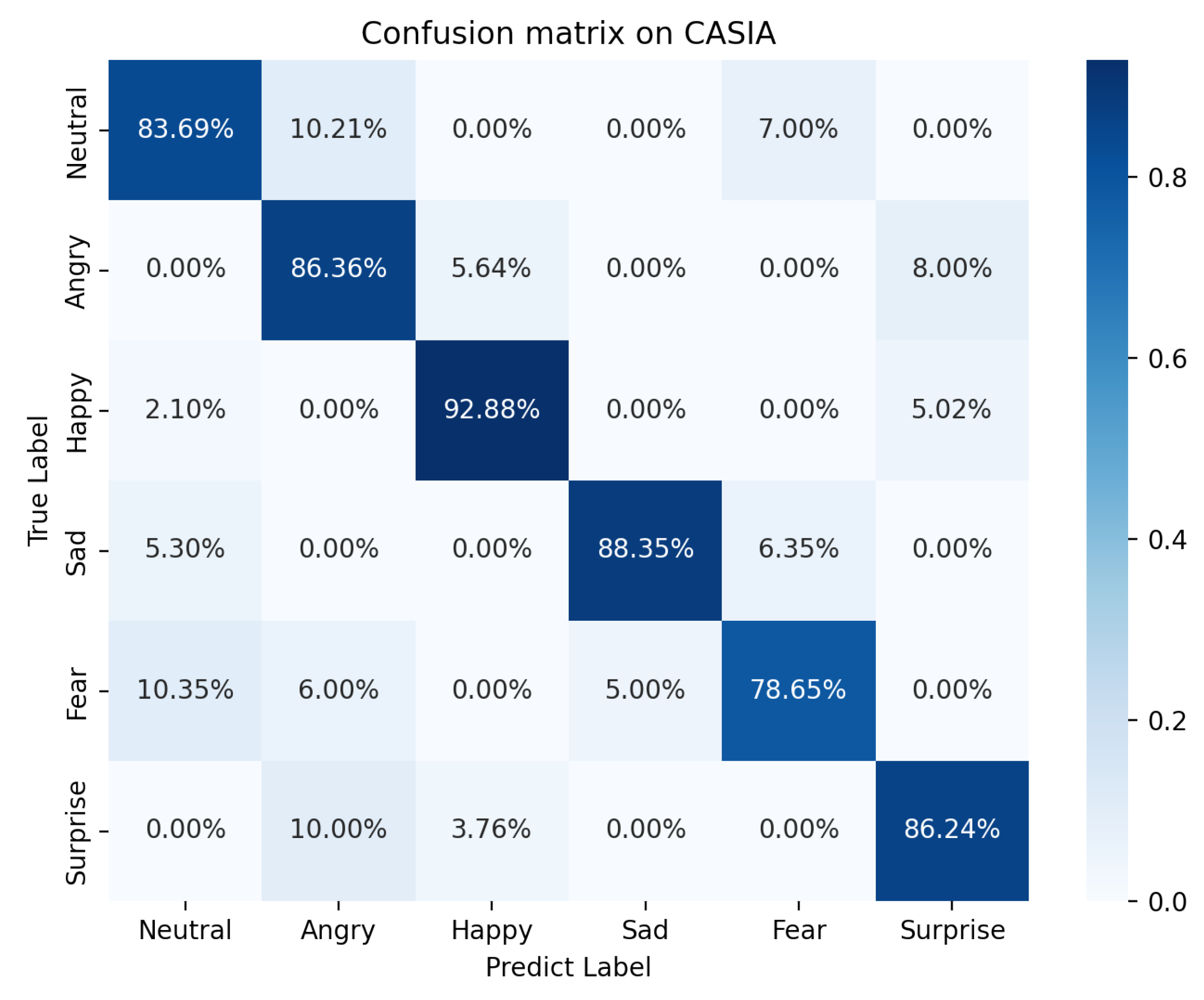
| DRSN-BiGRU | 86.24 | 78.65 | 88.35 | 92.88 | 86.36 | 83.69 |
| Model | Sad | Happy | Angry | Neutral |
|---|---|---|---|---|
| DCNN-LSTM | 77.46 | 81.21 | 81.63 | 78.53 |
| CNN-BiLSTM | 74.31 | 70.54 | 65.13 | 65.32 |
| DRN-BiGRU | 80.96 | 79.46 | 85.68 | 81.91 |
| DRSN-BiGRU | 86.00 | 90.20 | 83.52 | 84.59 |
| Model | Neutral | Angry | Fear | Joy | Sadness | Disgust | Surprise |
|---|---|---|---|---|---|---|---|
| DCNN-LSTM | 68.32 | 52.13 | 54.21 | 50.32 | 55.43 | 53.31 | 56.65 |
| CNN-BiLSTM | 71.65 | 47.89 | 45.68 | 61.86 | 55.59 | 48.87 | 59.54 |
| DRN-BIGRU | 70.23 | 58.56 | 62.78 | 64.45 | 59.35 | 52.31 | 60.34 |
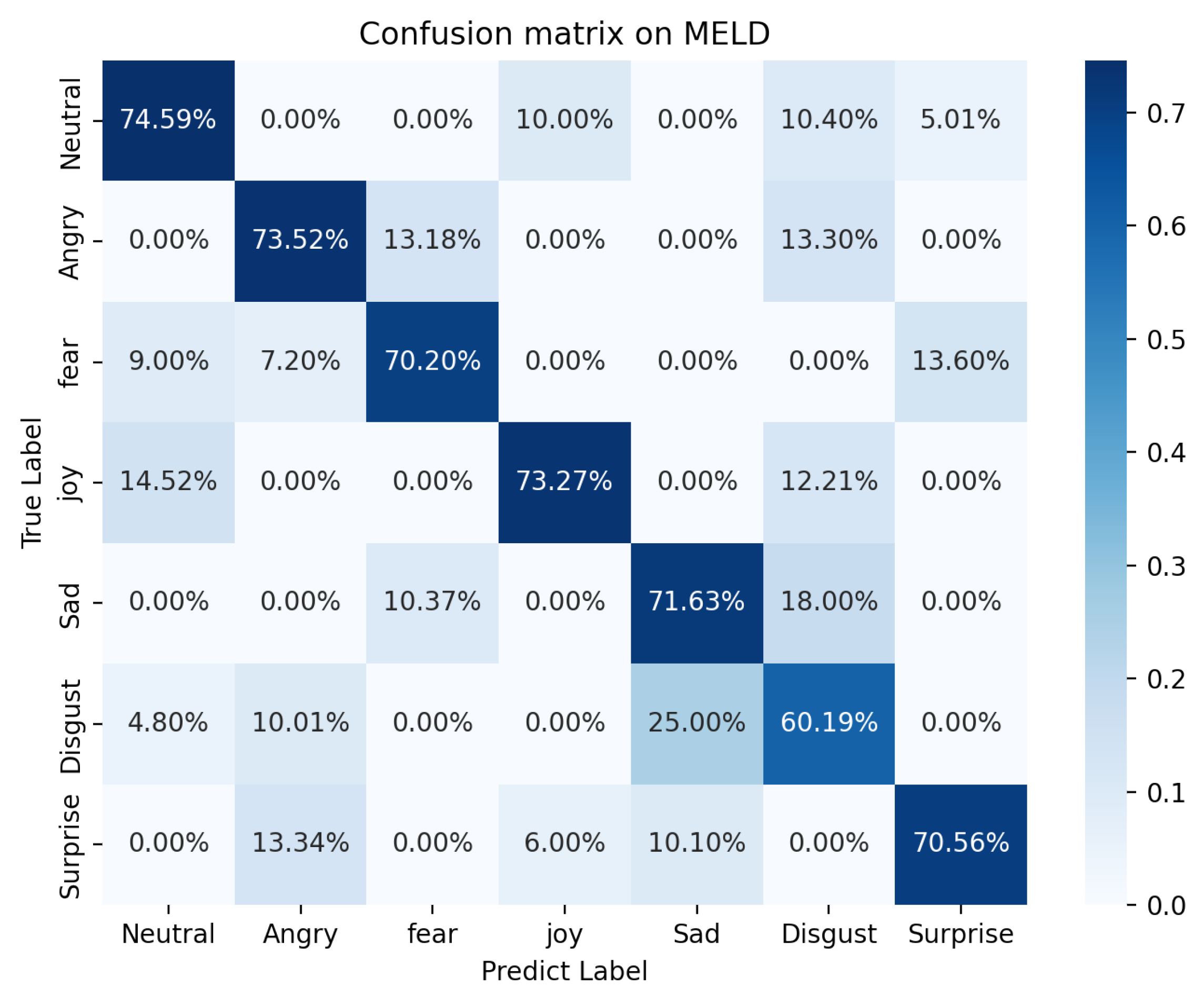
| DRSN-BIGRU | 74.59 | 73.52 | 70.20 | 73.27 | 71.63 | 60.19 | 70.56 |
Disclaimer/Publisher’s Note: The statements, opinions and data contained in all publications are solely those of the individual author(s) and contributor(s) and not of MDPI and/or the editor(s). MDPI and/or the editor(s) disclaim responsibility for any injury to people or property resulting from any ideas, methods, instructions or products referred to in the content. |
© 2023 by the authors. Licensee MDPI, Basel, Switzerland. This article is an open access article distributed under the terms and conditions of the Creative Commons Attribution (CC BY) license (https://creativecommons.org/licenses/by/4.0/).
Share and Cite
Han, T.; Zhang, Z.; Ren, M.; Dong, C.; Jiang, X.; Zhuang, Q. Speech Emotion Recognition Based on Deep Residual Shrinkage Network. Electronics 2023, 12, 2512. https://doi.org/10.3390/electronics12112512
Han T, Zhang Z, Ren M, Dong C, Jiang X, Zhuang Q. Speech Emotion Recognition Based on Deep Residual Shrinkage Network. Electronics. 2023; 12(11):2512. https://doi.org/10.3390/electronics12112512
Chicago/Turabian StyleHan, Tian, Zhu Zhang, Mingyuan Ren, Changchun Dong, Xiaolin Jiang, and Quansheng Zhuang. 2023. "Speech Emotion Recognition Based on Deep Residual Shrinkage Network" Electronics 12, no. 11: 2512. https://doi.org/10.3390/electronics12112512
APA StyleHan, T., Zhang, Z., Ren, M., Dong, C., Jiang, X., & Zhuang, Q. (2023). Speech Emotion Recognition Based on Deep Residual Shrinkage Network. Electronics, 12(11), 2512. https://doi.org/10.3390/electronics12112512