Anomalous Behavior Detection with Spatiotemporal Interaction and Autoencoder Enhancement

Abstract

To reduce the cargo loss rate caused by abnormal consumption behavior in smart retail cabinets, two problems need to be solved. The first is that the diversity of consumers leads to a diversity of actions contained in the same behavior, which makes the accuracy of consumer behavior identification low. Second, the difference between normal interaction behavior and abnormal interaction behavior is small, and anomalous features are difficult to define. Therefore, we propose an anomalous behavior detection algorithm with human–object interaction graph convolution and confidence-guided difference enhancement. Aiming to solve the problem of low accuracy of consumer behavior recognition, including interactive behavior, the human–object interaction graph convolutional network is used to recognize action and extract video frames of abnormal human behavior. To define anomalies, we detect anomalies by delineating anomalous areas of the anomaly video frames. We use a confidence-guided anomaly enhancement module to perform confidence detection on the encoder-extracted coded features using a confidence full connection layer. The experimental results showed that the action recognition algorithm had good generalization ability and accuracy, and the screened video frames have obvious destruction characteristics, and the area under the receiver operating characteristic (AUROC) curve reached 82.8% in the detection of abnormal areas. Our research provides a new solution for the detection of abnormal behavior that destroys commodity packaging, which has considerable application value.

1. Introduction

The integration of deep learning into traditional vending machines has led to the emergence of smart retail containers that provide a better consumer experience through open-door shopping and automated checkout processes. This innovation, however, has also given rise to abnormal consumption patterns. For enterprises, relying on visual recognition technology to achieve large-scale operation of smart retail cabinets is currently the most profitable choice. Consumption behavior recognition under smart retail is mainly achieved through commodity identification. The first step is to identify the customer’s purchase behavior for the movement trajectory of the product [1,2], and the second is to use the state and quantity of the product before and after the consumption behavior to identify the purchase behavior, for example, through the use of RFID [3] and image recognition [4,5] technology. Visual recognition schemes based on product identification can satisfy the requirement of identifying normal consumption action, but are far from meeting the challenge of abnormal consumption action recognition, including destructive action. Detecting these anomalous or abnormal consumption patterns has considerable economic value for enterprises. However, few algorithms for detecting abnormal action in intelligent retail design are available.

Anomaly detection refers to detecting instances of data that are significantly different from most ordinary instances. Anomaly detection is emphasized in areas such as data mining, computer vision, and deep learning. In recent years, the widespread adoption of deep learning has led to a series of deep anomaly detection methods, which have shown high practical performance in practical applications such as autonomous driving [6,7,8,9] and pathological detection [10,11]. According to the classification of supervision methods, anomaly detection methods based on deep learning can be divided into unsupervised, semi-supervised and weakly supervised methods. Among them, semi-supervised and weakly supervised methods are more mature. According to the anomaly learning method, the anomaly detection algorithm involves two learning methods: general normality feature learning and anomaly measure-related feature learning. General normality feature learning methods typically involve predictability modeling using autoencoders or generative adversarial networks (GANs) [12,13,14,15]. This provides guidance for anomalous action detection through anomalous features. The general normality feature learning method shows excellent performance in detecting anomalous instances; however, there is another side to this approach. Because the resulting network can easily be misled into generating instance data from multiple instances, this can negatively affect anomalous determination results.

An autoencoder network is a mainstream algorithm for video-based anomaly detection. Deng H. et al. [16] proposed a new T-S model composed of a teacher encoder and a student decoder, and introduced the “reverse distillation” paradigm because of the good performance of knowledge extraction within the unsupervised anomaly detection problem. Piergiovanni A. J. et al. [17] proposed a universal visual backbone which easily adapts a ViT architecture to videos. Due to the fact that smart retail cabinets often capture videos with only one customer, it is better to use action recognition algorithms instead of autoencoder networks to detect abnormal actions. In consumer–action recognition problems, human actions and human–object interactions have an impact on the final consumer action judgment results; therefore, the human–object interaction (HOI) algorithm [18,19,20,21] and video data-based action recognition algorithm can be used for consumer–action recognition. Most existing HOI detection approaches are instance-centric, and cannot capture complex HOI behavior with only appearance features; therefore, Wang T. et al. [22] proposed a novel and fully convolutional version of HOI, and a method wherein HOI detection is posed as the key to solving detection and grouping problems. However, most current action recognition algorithms focus more on human action, which leads to a lack of interactive action information. Meanwhile, the human–object interaction recognition algorithm that can use the interactive action information cannot process the video data, that is, the time information of the action cannot be used. Secondly, abnormal actions that include destroying commodities are the main reason for the commodity loss rate of smart retail cabinets. This is because this type of behavior involves the customer taking the product and damaging it, then putting the product back in its original place. Therefore, this kind of behavior can easily be identified as the customer not purchasing the commodity. This suggests that the boundary between abnormal and normal interaction behavior is difficult to define.

In this paper, we detect anomalous interactions in both commodity and customer behavior, i.e., vandalism that includes tearing up the packaging of the commodities/unscrewing the cap. Graph convolution with skeletal nodes can filter out a large amount of background redundant information. Inspired by [23], which defines graph nodes as the suggested regional features of objects through different frames, we propose a human–object interaction graph convolution network (HOI-GCN) to connect commodity nodes and skeleton nodes for interaction feature extraction. Zhian Liu et al. [24] proposed a novel hybrid framework with a combination of flow reconstruction and flow-guided frame prediction for video anomaly detection (HF2-VAD). The trained autoencoder network can reconstruct the normal behavior with a lower reconstruction error, and the reconstruction error for anomalous features is much larger. Reconstruction not only detects anomalous data, but also discovers the area wherein anomalies are located. Considering that the abnormal characteristics of the commodity are the key to distinguishing normal interaction behavior from abnormal interaction behavior, we use a confidence-guided difference enhancement module in the autoencoder networks to locate the damage area.

In conclusion, our contributions can be summarized as follows:

(1)

To recognize the abnormal action and obtain the corresponding video frames, we propose an action recognition strategy for interactive action. We construct a human–object interaction graph convolution network to extract the features of abnormal action, and to recognize actions using interaction and temporal characteristics.

(2)

To distinguish between abnormal interaction action and normal interaction action according to abnormal characteristics, we propose a confidence-guided anomaly enhancement module. We reconstruct less confident coded features using ordinary features with minimal similarity. At the same time, a perceptual loss function and a three-channel cosine similarity loss function are introduced to calculate the anomaly score of the image, and the division of the anomaly region is obtained.

2. Related Works

2.1. Anomaly Detection

Anomaly detection can be divided into GAN-based, CNN-based, and auto-encode-based detection. Morais R. et al. [25] proposed a method to model the normal patterns of human motion in surveillance videos, and used dynamic skeleton features for anomaly detection. Neelu Madan et al. [26] proposed a self-supervised block that can be applied in various advanced image and video anomaly detection algorithm frameworks. Feng et al. [27] proposed a multi-instance framework (MIST) and applied it to weakly supervised video anomaly detection (WS-VAD) to optimize a multiple-instance pseudo-label generator and self-guided attention-boosted feature encoder in MIST, using a self-training scheme. In the field of unsupervised learning, the earliest study using GAN-based predictability modeling was AnoGAN [28], proposed by Thomas Schlegl, which involved unsupervised learning of normal anatomical changes in the latent space of a normal sample through deep convolution GAN (DCGAN). The authors also designed two loss functions in the inference stage to calculate the difference between the generated and original graphs. The anomalous area was determined based on the weighted value and set threshold. Xia et al. [29] proposed two detection methods for fault detection and anomaly detection in semantic segmentation. They designed a network framework using the semantic segmentation module M combined with GAN networks to achieve the detection of anomalous items. In industrial anomaly detection, self-coding networks are the mainstream network. Memory modules and knowledge distillation models [30,31] are also widely used in self-coding networks for anomaly detection. Bae J. et al. [32] considered that the location and neighborhood information are ignored during the modeling of the current autoencoder network, which affects the distribution of normal features. They proposed a new modeling method, in which the conditional probability of a given neighborhood feature estimates the normal distribution and uses a multilayer perceptron network for modeling. To improve the speed of industrial anomaly detection, Kim D. et al. [33] proposed a method of fast adaptive patch memory (FAPM), eliminating unnecessary calculations, with good accuracy and speed.

2.2. Action Recognition

The basis of the solution can be divided into two parts: the first is relying on the extracted human body skeleton information for pose estimation, and the second is directly extracting the spatiotemporal features of the image for classification. Si Jie et al. [34] proposed a spatiotemporal graph convolution network (ST-GCN) based on the human skeleton, which represents the human skeleton node as a graph convolution node by modeling the dynamic bone, and uses a spatiotemporal convolution graph to express the multi-layer skeleton joint sequence. Furthermore, Li proposed an action–structure diagram convolutional network (AS-GCN), combining action links and structural links [35] with an ability to learn the characteristics of spatiotemporal actions simultaneously; they proposed that the recognition head and the future pose prediction head should be added together, and that the action model should be established through self-supervision. Zhang X. [36] used asymmetric correlation metrics and a more advanced context-aware graph convolution network (CA-GCN) to compute contextual information, further expanding the flexibility of the algorithm. Cheng et al. [37] proposed a new shift GCN (shift-GCN) for modeling a graph convolutional neural network with the human skeleton as a space-time map, and effectively reduced the computational complexity.

In the image-based spatiotemporal algorithm, the dual-stream expansion 3D convolutional network (I3D) proposed by Carreira et al. [38] achieves the learning of spatiotemporal features through expanding the convolutional layer and pooling the kernels from 2D to 3D. The dual-stream architecture composed of optical flow and RGB also enhances the network performance. Liu T. [39] proposed STILT, a dual-stream network for spatiotemporal interactive learning. STILT abandons the practice of separating spatial information and temporal information capture in the early dual-stream network, and pays greater attention to the strong complementarity and correlation of the spatial and temporal information in a video. It was able to effectively improve the recognition accuracy by establishing the interconnection of time flow and spatial stream. Ji Lin et al. [40] proposed a computationally efficient temporal shift module (TSM) combined with 2D CNN backbone networks, which makes it possible to achieve low-latency video recognition with edge devices. Limin Wang et al. [41] used an RGB difference and curved optical flow field as the network input and proposed a time period network (TSN) to simulate the long-term structure of an entire video for long-distance time series modeling as a new framework for action recognition.

3. Methods

Figure 1 and Figure 2 shows the flowchart of the algorithm, the action recognition based on human–object interaction graph convolution, and commodity damage feature detection under an autoencoder network based on a confidence-guided anomaly enhancement module. (1) The human–object interaction convolutional network is used to extract human action and interaction features. The position encoding and visual features are fused and fed into the interactive graph convolution and temporal interaction modules. (2) The corresponding encoder and decoder are obtained through network training. Confidence-guided difference enhancement is used to reconstruct latent features. The image generated by the encoder is compared with the original image at the pixel level and using depth semantics, and the damage calibration is obtained.

3.1. Action Recognition

3.1.1. Human–Object Interaction Feature Extraction

By observing videos of destructive action, we find that in the fragments in which the destructive behavior occurs, the hands are more related to the commodities in terms of movement and feature, especially during actions with obvious damage characteristics. Therefore, we encode the motion relationship between different frame objects. We define individual commodities and hands as our detection objects. Among these, the features of each object contain the center coordinate of the object along with its height, width and label as a vector, and we forward these to a multi-layer perception (MLP) network, yielding a d-dimensional feature and specifying the characteristics. Among these, the features of each object contain their own 2D coordinates and label information, taking the commodities as the key point.

Using a backbone CNN (e.g., ResNet-152 [42]), we can extract the image feature F of each object. The observations in [21] show that position embedding performs better concerning actions that directly describe the movements of objects, such as “put something” and “take something”.

However, this method performs worse concerning actions that are associated more with changes in the intrinsic properties of an object, such as “tearing”. For the t-frame video frame, the feature of object i is defined as $f_i^t$, which is calculated as follows:

$$f_i^t=GAP\left(Re{s}_h(RoI(F))\right)$$

(1)

3.1.2. Human–Object Interaction Graph Convolutional Network

We first define the node characteristics in the graph convolution. After obtaining the position-encoded features of a frame of the region of interest, we connect the position features of the node and the image features. The fusion of the two features is achieved with a 1 × 1 convolution kernel. Through this step, we will obtain the position of the object and the fusion characteristics $x_i^t$ of the image feature. The fusion features can be concatenated to form a feature of the object nodes in a graph, that is, the node matrix X.

When creating an interactive adjacency matrix for different objects in video frame t, a popular method is to use the position information of the objects to define the continuity between nodes. We define the coordinates of object i node as $U_i$. The relative coordinates are fed into the MLP layer, which is put into the corresponding point of the critical matrix as a proposal probability of size 1 between neighboring nodes. The adjacency matrix G of size N × N is obtained:

$${\mathrm{G}}_{i,j}^I=MLP(U_{i^t}-U_{j^t})$$

(2)

We used graph convolutional networks (GCNs) [43] to generate human–object interaction graphs. Graph convolution is different from standard convolution in that performing graph convolution is equivalent to performing message passing within the graph nodes. The output of the GCN is the updated feature of each object node; all the features of all object modes can be aggregated together for video classification. Formally, we can express the convolution of a layer of graphs as

$$P=GXW$$

(3)

where G represents an adjacency graph with N × N dimensions, X is the input feature of the object nodes in a graph with N × d dimensions, W is the weight matrix of d × d dimension layers, and the output of a graph convolutional layer Z still has N × d dimension. In our network, the W is the weight matrix of d × 1 dimension. It is used as the final classifier. Additionally, the output is the action class probabilities. We defined output P of the layer $G{\mathrm{rap}}^{\mathrm{I}}$ as

$$P_I=\sigma (G^{I}XW)$$

(4)

Finally, the output results after the graph convolution calculation were forwarded to the sigmoid function $\sigma$, which calculates the action class probabilities $P_I$ of size N.

3.1.3. Temporal Interaction Module

Trajectory characteristics in motion are critical to understanding video. When describing the motion, we use the temporal interaction module proposed in [21]. It computes the feature of the tracklet as $g(x_i^1,\dots ,x_i^T)$, and uses the non-local block [44] as the function h to combine and aggregate the information of the tracklets. It also uses the architecture of the 3D convolutional neural network proposed in [23] to perform 3D convolution operations and average pooling on the video sequence; subsequently, the feature $P_T$ of N dimension will be obtained. We stitch together the 3D features $P_D$ and tracklet features as follows:

$$P_T=\sigma (W_p^T[P_D,h(g{(x_i^1,\dots ,x_i^T)}_{i=1}^N)])$$

(5)

where [] represents the concatenation, and $W_p^T$ is used as a final classifier with cross-entropy loss. Finally, we combine the action class probabilities $P_I$ and temporal interaction probabilities $P_T$ by multiplying the probabilities, a method similar to previous work [45,46]. $P_F$ represents the final prediction vector of size N.

$$P_F=P_T\times P_I$$

(6)

3.2. Confidence-Guided Anomaly Detection

In the process of identifying anomaly action, the appearance of commodity packaging damage characteristics is the most reliable judgment for identifying the occurrence of sabotage; however, detecting and defining the damaged parts remains difficult, because the damage feature does not appear in normal consumption activities. The detection of damage features in the image is equivalent to the detection of out-of-detection (OOD) objects. In classification, OOD objects will be classified as any possible objects in the distribution. Based on action recognition, we performed semantic segmentation of commodity areas, and to simplify the complexity of the calculation, we classified the classification results of the segmentation model into $L=n+2$ types, that is, n commodities, customers, and backgrounds. Specifically, x is a video frame of size $w\times h$, and $L=\{1,2,\cdots ,L\}$ is a set of integers representing semantic labels. A pixel-level semantic label is obtained by sending image x to segmentation model M, where we use U-Net [47] for our segmentation model. At the same time, another type of U-Net [48] was used as autoencoder. It removed the last batch normalization and ReLU layers in the encoder instead of an L2 normalization layer, causing the feature to have a common scale.

After the segmentation was complete, we masked the background of the image before and after synthesis according to the segmented semantic label map, and processed the pixels in the background as black in order to reduce the interference generated by the background pixels during the comparison process, and to reduce the amount of computation required for training and testing.

3.2.1. Confidence-Guided Difference Enhancement Module

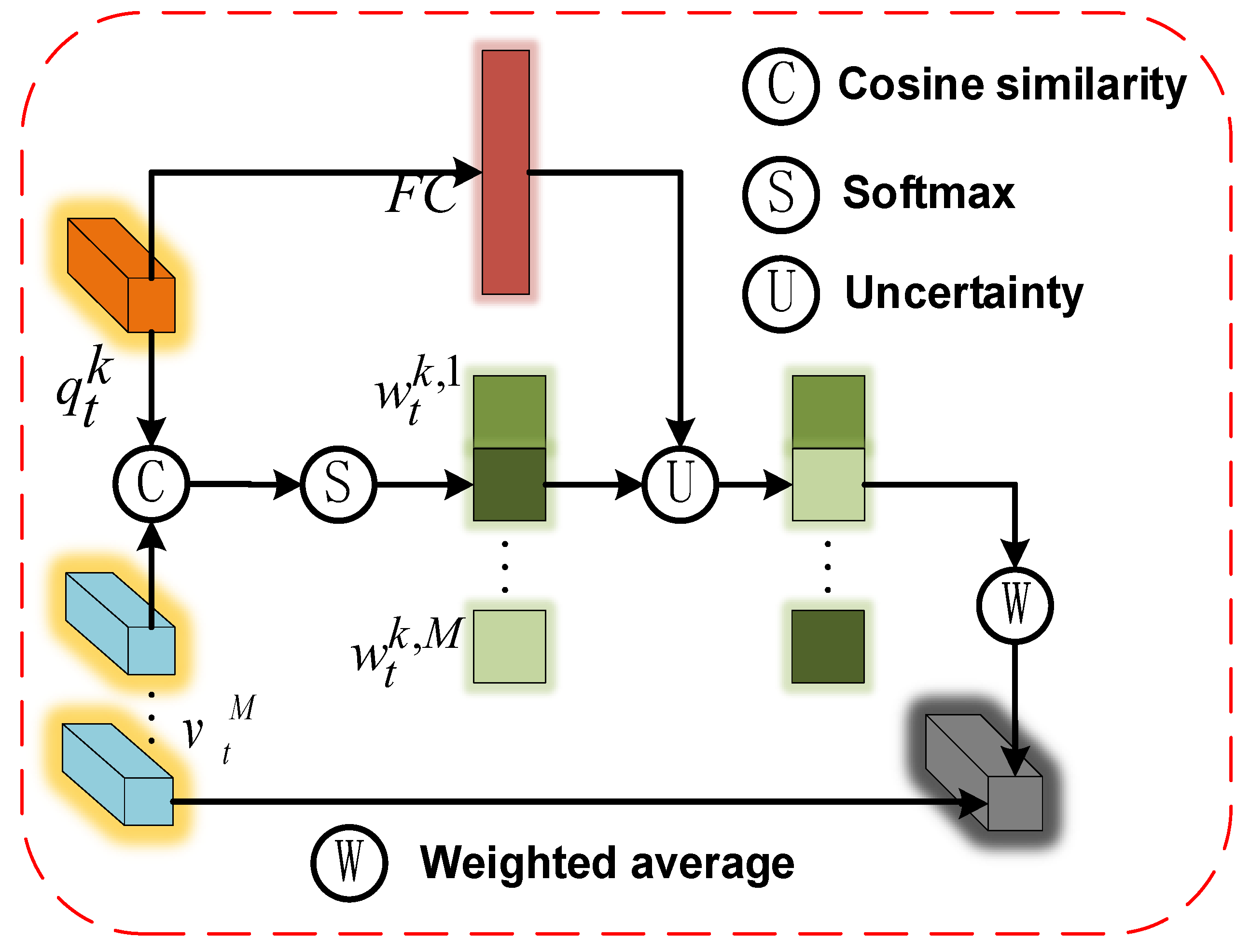
We use the encoder to extract features from the input video frame t to then generate the query map $q_t$. The size of it is $H\times W\times C$, where $H,W, \mathrm{and} C$ are height, width, and the number of channels. $q_t^k\in {ℝ}^C\left(k=1,\cdots K\right)$ denotes individual queries of size $1\times 1\times C$ in the query map, where $K=H\times W$. We also use the memory items, which contain M items recording various normal data. The normal data were generated by the encoder of the normal frame containing the people and commodities. The normal frame of the customer was captured at the beginning of the video. We denote the item in the memory using $v_m\in {ℝ}^C(m=1,\cdots M)$. We calculate the cosine similarity between each query $q_t^k$ and all items $v_m$ in the memory to obtain a two-dimensional correlation graph of size M × K. By performing a global softmax function, the probability $w_t^k$ of $q_t^k$ matching the $v_m$ is obtained. Figure 3 shows the flowchart of the confidence-guided difference enhancement module.

$$w_t^{k,m}=softmax\left[\frac{exp({(v_m)}^T{q}_t^k)}{{{\displaystyle \sum }}_{m^{\prime }=1}^{M}exp\left({\left(v_{m^{\prime }}\right)}^T{q}_t^k\right)}\right]$$

(7)

We add a fully connected layer to $q_t^k$ as a confidence branch of the network, measuring the confidence level of the network evaluation. When the network confidence level is low, we reverse the original weight $w_t^{k,m}$ in succession to obtain features that are more different from the original image. By guiding the decoder to direct the anomalous features in the direction in which they are least similar, the difference can be increased. The transformed feature map and query features are assembled into the decoder. The formula is as follows.

$${\widehat{v}}_t^k=\{\begin{array}{c}{\displaystyle {\displaystyle \sum }_{m^{\prime }=1}^M}{w}_t^{k,m^{\prime }}{v}_{m^{\prime }} if FC(q_t^k)<\delta \\ {\displaystyle {\displaystyle \sum }_{m^{\prime }=1}^M}\left(1-w_t^{k,m^{\prime }}\right)v_{m^{\prime }} if FC(q_t^k)\ge \delta \end{array}$$

(8)

To train a fully connected layer of confidence, we only feed normal items into the fully connected layer. We denote the similarity of normal feature $q_t^k$ to memory item ${\mathrm{v}}_m$ using $w_m^k$. We define y as the target probability distribution of the input normal features. The target probability distribution can give the network “hints”. The confidence c denotes the probability that a query belongs to the memory items. Through training, normal features attain higher confidence in fully connected networks. The formula is as follows:

$$w_t^{k^{\prime },m}=\left(1-c\right)·w_t^{k,m}+c·y_t^{k,m}$$

(9)

We calculate the task loss using the prediction of negative log likelihood. To prevent the network from always choosing to receive the entire ground truth for minimizing the loss function, we add a binary cross-entropy loss function and balance the two losses using a hyperparameter λ; the loss function is as follows:

$${ℒ}_c=\lambda \left({\displaystyle \sum }_{m=1}^M{y}_t^{k,m}\log \frac{1}{w_t^{k^{\prime },m}}\right)+\left(1-\lambda \right)\log \left(\frac{1}{c}\right)$$

(10)

3.2.2. Comparison of Shallow Features

In the process of calculating the characteristic value of commodity damage, not all abnormal feature values have an equal impact on the judgment results. If only the single feature value of each pixel is compared in the process of comparing the image, the calculation result will produce a large error, which is not conducive to the overall understanding of the damaged area. This is because the production of abnormal features of commodities and the destruction of commodity packaging have a strong causal relationship. Therefore, we synthesized the changes in hand nodes in the n frames before and after the selected video frame, and performed pixel-level feature vector stitching. We let the horizontal and ordinate changes of the nodes of the two adjacent frames be expressed as $K_{x_m}^p,K_{y_m}^p$, specifying that the left and down movements are negative values, where p represents the hand, and m is the m-frame in n frames.

$$\stackrel{\wedge }{\theta }=\arctan \left({\displaystyle \sum }_{m=2}^n{K}_{x_m}^p,{\displaystyle \sum }_{m=2}^n{K}_{y_m}^p\right)$$

(11)

We stitched the pixels in position according to the size of the frame of the selected video frame $\mathrm{w}\times \mathrm{h}$, where $f_M^i$ is the feature vector of the RGB channel at the $i^{th}$ pixel position of the last layer output of the segmentation model M. By stitching the feature values in the $\widehat{\theta }$ direction, we filled the rest of the video frame $\widehat{\theta }$ with black according to w×h, and the feature vector of the stitching $f_{{\widehat{\theta }}_w}^i$, where $\lfloor ,\rfloor$ represents the splicing of pixels. When the sum value of the motion coordinates is small, we skipped the area aggregation module and directly compared the pixel-level features of each point.

$$f_{{\widehat{\theta }}_w}^i=\lfloor f_{{\widehat{\theta }}_w}^{i_1},f_{{\widehat{\theta }}_w}^{i_2},\dots ,f_{{\widehat{\theta }}_w}^{i_{h+w}}\rfloor$$

(12)

Subsequently, for regions with large outliers, we compared the cosine distance de-fined on the intermediate feature of each element in the region:

$$S_n^{\left(i\right)}=F\left(x,r\right)=1-\langle \frac{f_M^i\left(x\right)}{\parallel f_M^i{\left(x\right)\parallel }_2},\frac{f_M^i\left(r\right)}{\parallel f_M^i{\left(r\right)\parallel }_2}\rangle$$

(13)

where $\langle ·,·\rangle$ is the inner product of two vectors.

3.2.3. Comparison of Deep Features and Fusion

Although shallow features can make good use of pixel-level information, the expression of higher features is missing, and the global features of the broken area are not expressed. We expressed the semantic differences between the segmentation map and the composite map by calculating the perceived loss of each pixel. Furthermore, by using the semantic differences between abnormal objects in the composite image, we can compare the deep features of each pixel.

The pixels of the original video frame are defined as $f_M^i(x)$, and the pixels of the composite video frame are defined as $f_M^i(x)$, where $F^{\left(i\right)}$ represents the elements of layer i in the N layer of the VGG network, which are normalized between [0, 1]. The perceived difference expression is as follows:

$$D(x,r)={\displaystyle \sum }_{i=1}^N\frac{1}{M_i}{\parallel F^{\left(i\right)}\left(f_M^i(x)\right)-F^{\left(i\right)}\left(f_M^i(r)\right)\parallel }_1$$

(14)

Subsequently, we synthesized the differences of the deep and shallow layers of the same position, and assigned different weights to the deep features and shallow feature differences of each node, wherein we define the weight parameter as ${\lambda }_S$, ${\lambda }_D$. Finally, depending on the presence or absence of abnormal areas in the commodity, a fine judgment of the damage to the commodity can be made. The final synthetic difference is $SD$, which can be determined using the following formula:

$$SD={\lambda }_S·S_n+{\lambda }_D·D$$

(15)

4. Experimental Results and Analysis

4.1. Experimental Platform and Dataset

The following platforms were used in this experiment: Windows 11; Graphics: NVIDIA GeForce GTX1650; Server: Nine days of ascension, Baidu PaddlePaddle. We used the Pytorch deep learning framework, PaddlePaddle 2.3 networking framework, and Python 3.8 to build the network model.

Because the commodity destruction video dataset is still blank in the public dataset of anomaly detection, the actual situation of the popular public dataset of anomaly detection and the abnormal behavior of consumption are quite different. To ensure the validity and accuracy of the experiment, it was conducted using homemade datasets. For each video, only a single customer consumes, excluding multiple people consuming at the same time. The consumer is in a bright environment. Additionally, all the customer’s behavior is in the area that can be monitored by the camera, and there is no malicious occlusion and other problems in the customer’s consumption behavior. Since the container door is transparent, the camera is placed above the inside of the container, and the shooting area is directly facing the retail container door. The inside of the smart retail container is equipped with light strips. This ensures that customers are also under a good light source when consuming at night. The video starts recording when the customer opens the door, and stops recording when the customer closes the door.

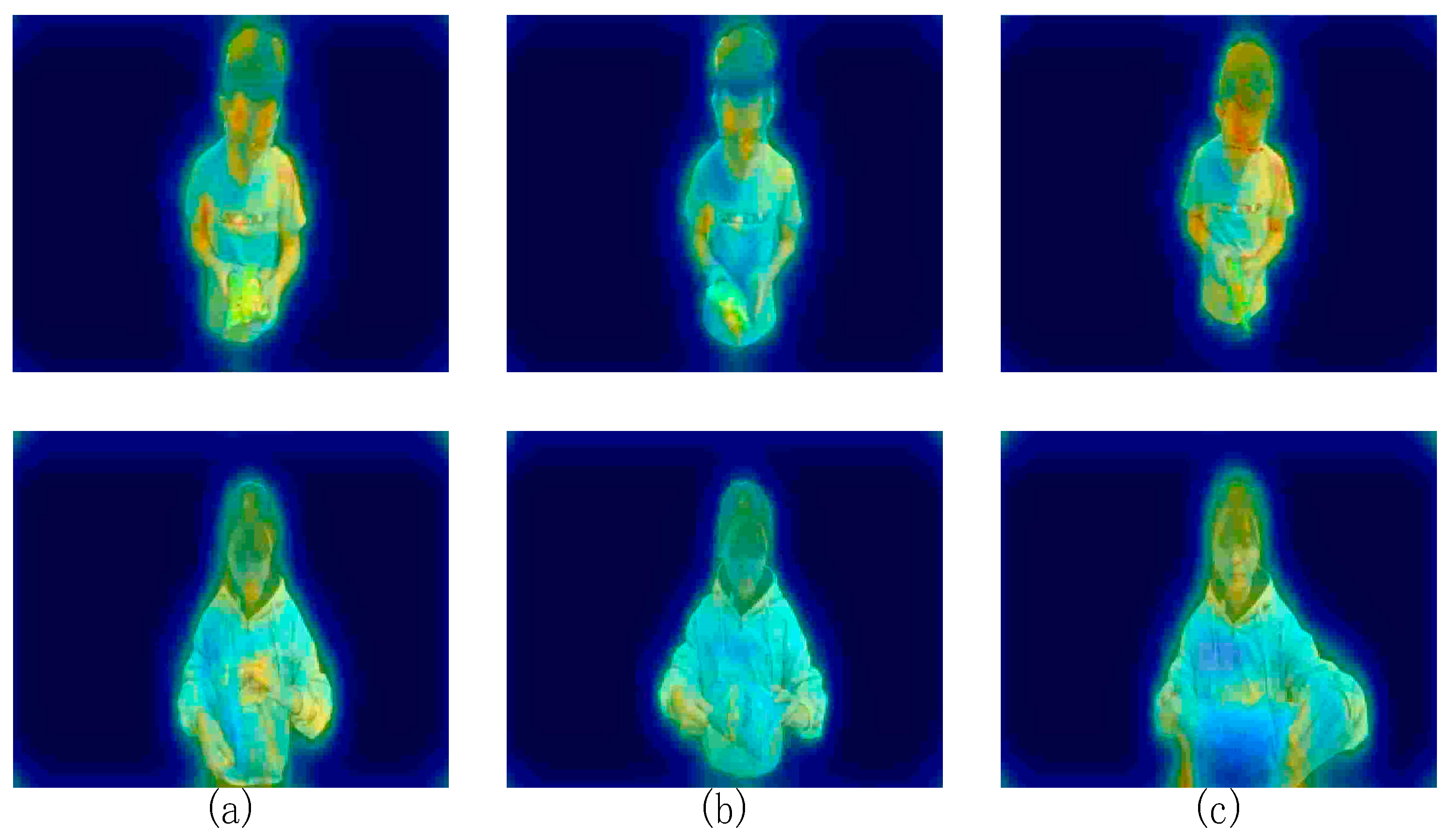
We divided consumer behavior into four behavioral categories (buying, not buying, drinking water, and tearing up packaging) and included three types of commodities (potato chips, biscuits, and drinks). The commodities used did not include those with transparent outer packaging. We also tested our algorithm on the MVTec AD dataset shown in Figure 4. Figure 5 shows the four behavioral data points, and

Table 1. Details of video datasets used in our experiments.

Actions	Train	Resolution	Commodity	Test
Destory	397	1280 × 720	4	44
Purchase	891	1280 × 720	7	98
No purchase	412	1280 × 720	7	45
Drink	372	1280 × 720	3	41

lists the details of our dataset. This is a dataset that mimics industrial production scenarios and is mainly used for unsupervised anomaly detection. The dataset contains five textures and ten objects from different domains.

4.2. Comparision with State-of-the-Art Models

4.2.1. Action Recognition

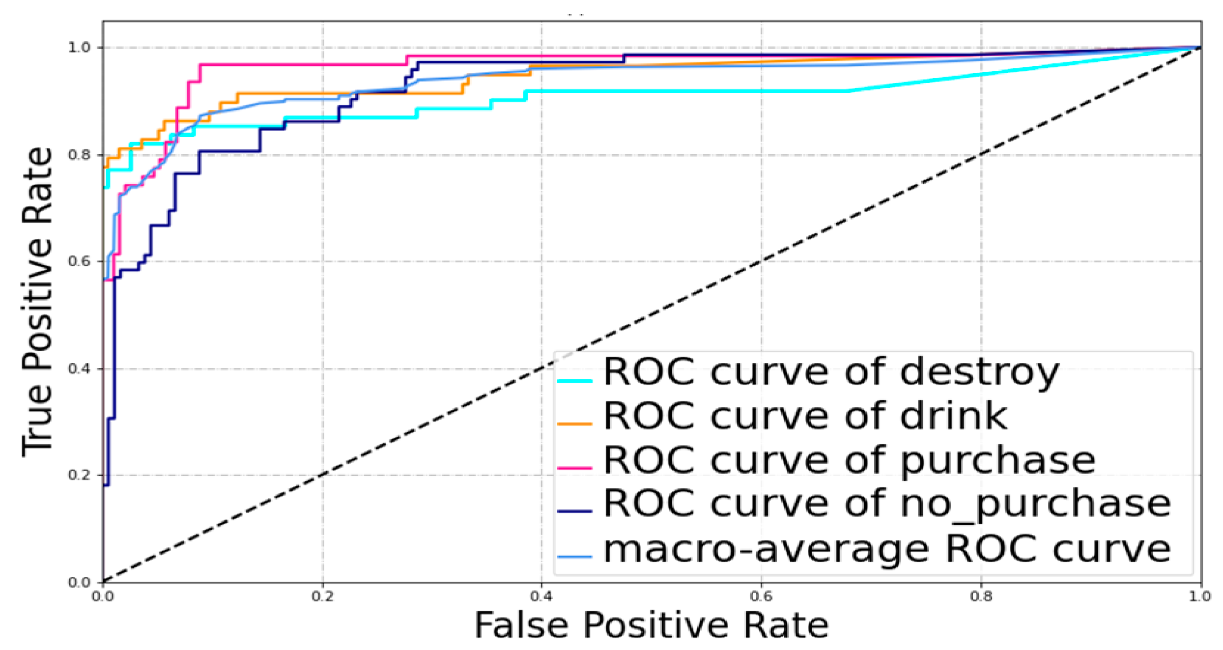
To verify the effectiveness of the human–object interaction graph convolutional network, a comparative experiment was designed to compare two indicators: the area under the curve (AUC), and the receiver operating characteristic curve (ROC). We plotted the ROC curve for each action in the selected algorithm and used the AUC as an indicator to test the generalization ability of the selected model. The parameters in the code were set to 50 epochs with a batch size of 64. Figure 6 presents the ROC curve.

Table 2. Comparison experiment of AUC and Top-1 accuracy of consumer behavior recognition with various algorithms.

Algorithm	Input	AUC	Top-1 Accuracy
ST-GCN	Skeleton	0.76	0.65
ST-GCN(AT)	Skeleton	0.81	0.74
MS-G3D [50]	Skeleton	0.86	0.81
Timesformer	RGB	0.87	0.84
TSN	RGB	0.92	0.85
I3D + STIN + OIE + NL [21]	RGB	0.84	0.82
Ours	RGB	0.90	0.86

lists the AUC calculation indicators, the accuracy of the model detection, and the time spent on 57 videos for each network. The video is recorded from a top-down perspective, and this greatly interferes with the performance of the graph convolutional network based on human skeletons. We use the timesformer structure proposed by Gedas Bertasius et al. [49] to understand the video, which is completely based on the self-attention mechanism and does not use the convolutional structure. The timesformer structure not only enhances the spatiotemporal modeling ability of the network, but also reduces the complexity and computational load of the network.

The videos from the visual system are important for identifying results. When the camera’s shooting area does not cover the main parts of the human body or occludes too much, the performance of the network based on skeleton nodes will be seriously degraded. The quality of the image taken has a significant impact on the network, wherein the input data is RGB. The more video frames the visual system takes per second of an action, the more data we will obtain. Thus, our vision system for shooting video uses an image resolution of 1280 × 720 and an fps of 27. The influence of the visual system within the network is minimized.

4.2.2. Anomaly Segmentation Method on MVTec AD

We used AUROC and FPR95 as our evaluation indicators in anomaly segmentation methods. Furthermore, we represent the abnormal as TP at the broken part of the commodity, and as FP if the normal area is marked as abnormal, where i represents the true value, j represents the predicted value, and p_ij represents the number of pixels that predict i as j.

In the comparison of public datasets, our algorithm has more descriptions of motion characteristics, which is useless in industrial datasets. Our algorithm tends to increase the error according to the labels. That is, we can decode the abnormal characteristics of the product according to the human body or background characteristics through the confidence-guided difference enhancement module, so as to widen the difference between the abnormal characteristics of the product and the product. This does not work in some industrial data sets. Additionally, some of the perceptual loss functions perform poorly in some feature textures.

Therefore, we only tested some data with two labels. Although our algorithm still has shortcomings compared to the current algorithm, it shows better results in some complex datasets.

Table 3. Comparison between industrial anomaly detection methods.

AUROC/Method		MemSeg [51]	FastFlow [52]	Ours
Metal Nut	Pixel	99.3	97.9	96.5
	Image	100	100	98.3
Hazelnut	Pixel	97.8	98.1	98.8
	Image	100	100	99.9
Pill	Pixel	99.5	99.2	97.5
	Image	99.3	99.6	99.8
Toothbrush	Pixel	99.2	97.9	96.8
	Image	99.7	99.3	99.8
Bottle	Pixel	99.1	98.2	96.3
	Image	100	99.6	97.1

presents the results.

4.2.3. Video Frame Selection

Our action recognition algorithm defines the t-frame as the central frame, and obtains the probability distribution of the destruction. We use the probability of destruction as the selection weight for the t-frame. The classical algorithms for video frame selection include the clustering algorithm, optical flow algorithm, and temporal difference method. Video frame selection aims to obtain the most representative video frames. In the present study, we compared the video frame selection algorithm based on human–object interaction with the above classical algorithm. We used a prediction of correct keyframes (PCK) indicator; PCK is the proportion of correctly estimated video frames within the keyframes. In the algorithm, we set n to 29 and randomly took 140 videos as our detection videos, wherein the total number of video frames and the number of keyframes are average. The total number of frames is 5350.

Table 4. Comparison experiment of PCK on various methods.

Method	Key Frames	PCK (%)
Temporal difference method	77	42.1
Optical flow method	297	12.2
Clustering method	336	53.3
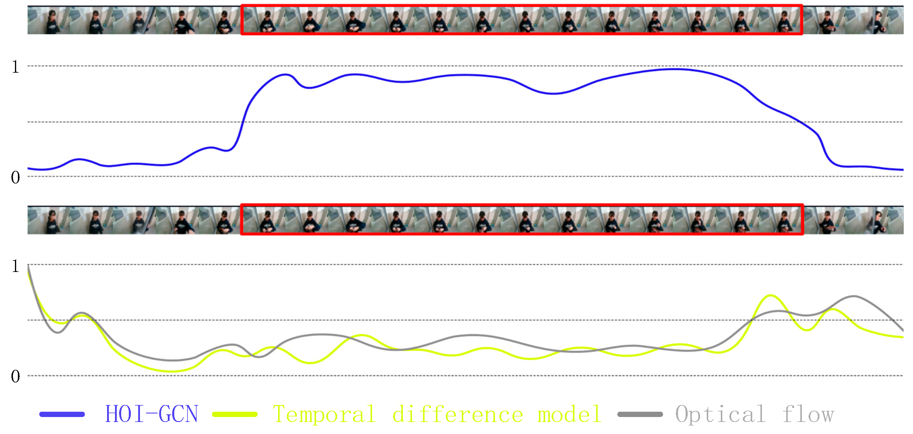
Ours	287	82.4

presents the results. It can be observed from the table that our screening of video frames of destructive action is more effective. The optical flow method performs poorly in experiments; the reason for the poor performance is that the brightness of the opening and closing door changes significantly, due to which the optical flow change when the action occurs is relatively small. Thus, the video frame containing the destruction is not easy to detect. The clustering method has evident differences in the selection effect for different videos, because the optimal threshold selection of different videos is different. After repeating the experiments a few times, we set the threshold to 0.89. Figure 7 presents the experimental results. To detect the broken features, the best keyframe extracted should be the intermediate frame wherein each action occurs. In the experiment, we found that keyframe extraction based on interaction extracts all the keyframes containing related actions and similar actions, which makes the number of keyframe extractions extremely large and scattered, which is not conducive to the detection of broken features. With the addition of motion analysis, the number of keyframes was significantly reduced, and the selected keyframes were concentrated near the intermediate frame in which the action occurs.

4.3. Ablation Studies

Effectiveness of Confidence-Guided Difference Enhancement Module and Fusion

In the proposed network, one of the core components of the methodology, confidence-guided anomaly enhancement, enhances differences in order to guide the detection of anomalous features. At the same time, the fusion of deep and shallow features provides more comprehensive information for the calculation of anomaly scores. To investigate the effectiveness of confidence-guided anomaly enhancement modules and feature fusions, we study the ablation of six variants: (1) confidence-guided anomalous enhancement modules with shallow features; (2) confidence-guided anomaly enhancement module with deep features; (3) shallow features; (4) deep features; (5) fusion; (6) confidence-guided anomalous enhancement modules with fusion. During the experiment, because the synthesis of the background was unnecessary, we used a U-net segmentation network to separate the consumer’s upper body and the commodity, and the remaining space was filled with black.

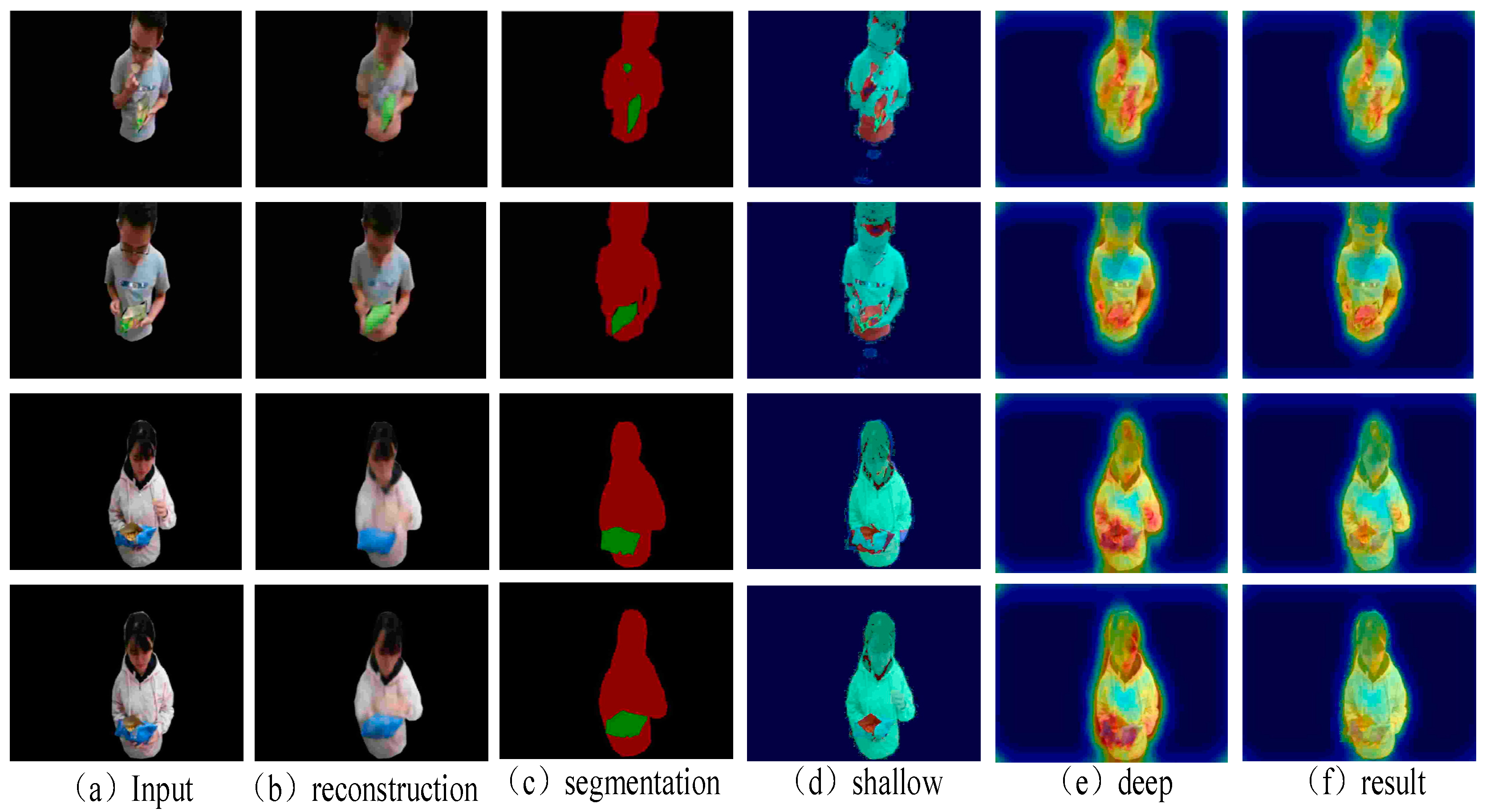
We compared our algorithm with two methods. Compared with the uncertainty of the last layer of the segmented network, we obtained better results for deep and shallow feature fusion. In the decoding process, when the decoder map of the human body area is compared with the original map, differences can be observed in some nodes, especially after the appearance of the damaged area. The perception difference often expands the size of the abnormal area during the detection process, and thus the accuracy of anomaly detection is reduced. We can converge the detection range of the perception difference by fusing shallow features, and the damaged area can be delineated and distinguished more accurately. Figure 8 displays the experimental figure. Evidently, the result map is more accurate for the boundary definition of some anomalous areas relative to the deep difference, especially for anomaly detection in commodity areas.

In the perceptual difference calculation, we assigned different weights to the perceived loss function of the network in different dimensions of the five layers of the VGG network. We found that although the perceived loss of the fifth layer is theoretically the best, experimentally, the perceived loss of the fourth layer has greater accuracy for the division of the image damage area. Therefore, the order of our assignment of weights from the largest to smallest is as follows: fourth layer, fifth layer, third layer, second layer, and first layer. To verify the effectiveness of the fusion strategy, we detected the deep and shallow features individually and compared their effects after fusion.

Table 5. Ablation studies of the confidence-guided difference enhancement modules and the fusion of multi-layered differences. C stands for confidence-guided difference enhancement modules, S for shallow difference, and F for deep difference.

C	S	F	AUROC
	✓		35.9
		✓	37.2
✓	✓		40.3
✓		✓	42.7
	✓	✓	71.8
✓	✓	✓	82.8

presents the algorithm results for the modules.

4.4. Analysis of Results

Image regeneration inevitably produces errors, and undamaged commodities may have damaged features due to errors in rebuilding features. We use different fusions ${\lambda }_S$ and ${\lambda }_D$ in three ratios (0.3, 0.6; 0.2, 0.7; and 0.1, 0.8) because the difference in network synthesis is evident for shallow features, and its difference is small for deep features. Therefore, we randomly assigned the above three proportions to each image. Figure 9 presents the anomaly detection for normal images. The fusion of visible deep and shallow features effectively suppresses the difference generated by synthesis in the commodity area.

The changes in and deformation of objects may generate abnormal features when no destructive action occurs. This has an impact on the abnormal detection. However, as shown in Figure 9, we caused changes in and the deformation of the object through flipping and extruding. The wrong delineation of the zone did not occur. Firstly, these characteristics are present in normal purchases, due to the inevitable changes in and deformation of objects when grasping. As a result, the confidence of the features encoded by such objects is very high throughout the FC layer, that is, the memory module contains similar features. The network reconstructs in the direction most similar to the input feature. Secondly, the detection of anomalies caused by perceptual differences occurs in the features after convolution. The comparison of such deep features is based on whether the features belong to the category of the region in which the segmentation map is located, as has been shown in Figure 8. When the shallow comparison module compares the original image with the restricted image at the pixel level, the detected anomalies only detect the area with a very large difference. For the image reconstructed in the most similar direction, the shallow comparison module cannot play a large role. Therefore, changes in and the deformation of objects will not affect the delineation of abnormal regions.

5. Discussion

In this paper, we propose a method of behavior recognition based on customer behavior and commodity information, which is quite different from methods in previous works focused on SKUs. Because of the small size of the smart retail container, we set the consumption object as a single customer. This makes our algorithm unsuitable for cases of group consumption such as unmanned convenience stores. The abnormal behavior detection algorithm based on damage features consists of two parts. We first identify the actions in the video in order to achieve action recognition in the video. In addition to the usual two actions of either buying or putting the undamaged commodity back, we also defined the behaviors of tearing up packaging to take food and unscrewing the lid of a bottle. If we detected the customer destroying the commodities, we extracted the key frames of this event, detected the damaged part of the commodity, and delineated the abnormal area.

The proposed action recognition strategy combines interaction features and temporal features for consumer behavior recognition, and has excellent detection accuracy and generalization ability. Our action recognition strategy not only considers the temporal characteristics of the action, but also considers the interaction characteristics in a single video frame. The results show that the action recognition module designed using an interactive graph is superior to alternative action recognition algorithms, and the selected video frames show obvious damage characteristics. The ROC curve illustrates the good generalization ability of our algorithm.

The confidence-guided anomaly enhancement module can greatly increase abnormal features and reconstruct normal features well. Compared with other anomaly detection networks based on autoencoder network, our network has added a confidence-guided difference enhancement module and a comparison module. Ablation experiments have proved that the additions of our module are effective. Our strategy of combining a shallow feature comparison network of motion information with the fusion of deep and shallow features can alleviate false alarms caused by the reconstruction process. Based on our results, we can conclude that anomalous features can be precisely divided. Finally, based on the presence or absence of abnormal features of the product, we can accurately identify abnormal behavior.

References

1. Kim, D.H.; Lee, S.; Jeon, J.; Song, B.C. Real-time purchase behavior recognition system based on deep learning-based object detection and tracking for an unmanned product cabinet. Expert Syst. Appl. 2020, 143, 113063. [Google Scholar] [CrossRef]
2. Liu, L.; Cui, J.; Huan, Y.; Zou, Z.; Hu, X.; Zheng, L. A Design of Smart Unmanned Vending Machine for New Retail Based on Binocular Camera and Machine Vision. IEEE Consum. Electron. Mag. 2021, 11, 21–31. [Google Scholar] [CrossRef]
3. Ramzan, A.; Rehman, S.; Perwaiz, A. RFID technology: Beyond cash-based methods in vending machine. In Proceedings of the 2017 2nd International Conference on Control and Robotics Engineering (ICCRE), Bangkok, Thailand, 1–3 April 2017; IEEE: Piscataway, NJ, USA; pp. 189–193. [Google Scholar]
4. Zhang, H.; Li, D.; Ji, Y.; Zhou, H.; Wu, W. Deep learning-based beverage recognition for unmanned vending machines: An empirical study. In Proceedings of the 2019 IEEE 17th International Conference on Industrial Informatics (INDIN), Helsinki, Finland, 23–25 July 2019; IEEE: Piscataway, NJ, USA; Volume 1, pp. 1464–1467. [Google Scholar]
5. Liu, C.; Da, Z.; Liang, Y.; Xue, Y.; Zhao, G.; Qian, X. Product Recognition for Unmanned Vending Machines. IEEE Trans. Neural Netw. Learn. Syst. 2022, 1–14. [Google Scholar] [CrossRef] [PubMed]
6. Lu, Y.; Yu, F.; Reddy, M.K.K.; Wang, Y. Few-shot scene-adaptive anomaly detection. In Proceedings of the Computer Vision–ECCV 2020: 16th Europe-an Conference, Glasgow, UK, 23–28 August 2020; Proceedings, Part V 16. Springer International Publishing: Berlin/Heidelberg, Germany, 2020; pp. 125–141. [Google Scholar]
7. Yao, Y.; Wang, X.; Xu, M.; Pu, Z.; Atkins, E.; Crandall, D. When, where, and what? a new dataset for anomaly detection in driving videos. arXiv 2020, arXiv:2004.03044. [Google Scholar]
8. Yao, Y.; Xu, M.; Wang, Y.; Crandall, D.J.; Atkins, E.M. Unsupervised traffic accident detection in first-person videos. In Proceedings of the 2019 IEEE/RSJ International Conference on Intelligent Robots and Systems (IROS), Macau, China, 3–8 November 2019; IEEE: Piscataway, NJ, USA, 2019; pp. 273–280. [Google Scholar]
9. Kendall, A.; Gal, Y. What uncertainties do we need in bayesian deep learning for computer vision? Adv. Neural-Form. Process. Syst. 2017, 30. [Google Scholar]
10. Li, Y.; Xu, C.; Han, J.; An, Z.; Wang, D.; Ma, H.; Liu, C. MHAU-Net: Skin Lesion Segmentation Based on Multi-Scale Hybrid Residual Attention Network. Sensors 2022, 22, 8701. [Google Scholar] [CrossRef] [PubMed]
11. Shvetsova, N.; Bakker, B.; Fedulova, I.; Schulz, H.; Dylov, D.V. Anomaly detection in medical imaging with deep perceptual autoencoders. IEEE Access 2021, 9, 118571–118583. [Google Scholar] [CrossRef]
12. Zenati, H.; Foo, C.S.; Lecouat, B.; Manek, G.; Chandrasekhar, V.R. Efficient gan-based anomaly detection. arXiv 2018, arXiv:1802.06222. [Google Scholar]
13. Donahue, J.; Krähenbühl, P.; Darrell, T. Adversarial feature learning. arXiv 2016, arXiv:1605.09782. [Google Scholar]
14. Zhu, J.-Y.; Park, T.; Isola, P.; Efros, A. Unpaired image-to-image translation using cycle-consistent adversarial networks. In Proceedings of the IEEE International Conference on Computer Vision (ICCV), Venice, Italy, 22–27 October 2017; pp. 2223–2232. [Google Scholar]
15. Arjovsky, M.; Chintala, S.; Bottou, L. Wasserstein Generative Adversarial Networks. In Proceedings of the 34th International Conference on Machine Learning, Sydney, Australia, 6–11 August 2017; pp. 214–223. [Google Scholar]
16. Deng, H.; Li, X. Anomaly Detection via Reverse Distillation from One-Class Embedding. In Proceedings of the IEEE/CVF Conference on Computer Vision and Pattern Recognition, New Orleans, LA, USA, 18–24 June 2022; pp. 9737–9746. [Google Scholar]
17. Piergiovanni, A.J.; Kuo, W.; Angelova, A. Rethinking Video ViTs: Sparse Video Tubes for Joint Image and Video Learning. arXiv 2022, arXiv:2212.03229. [Google Scholar]
18. Liao, Y.; Liu, S.; Wang, F.; Chen, Y.; Qian, C.; Feng, J. PPDM: Parallel Point Detection and Matching for Real-Time Human-Object Interaction Detection. In Proceedings of the 2020 IEEE/CVF Conference on Computer Vision and Pattern Recognition (CVPR), Seattle, WA, USA, 13–19 June 2020; IEEE: Piscataway, NJ, USA, 2020. [Google Scholar]
19. Zhong, X.; Ding, C.; Qu, X.; Tao, D. Polysemy Deciphering Network for Robust Human–Object Interaction Detection. Int. J. Comput. Vis. 2021, 129, 1910–1929. [Google Scholar] [CrossRef]
20. Hou, Z.; Yu, B.; Qiao, Y.; Peng, X.; Tao, D. Affordance transfer learning for human-object interaction detection. In Proceedings of the IEEE/CVF Conference on Computer Vision and Pattern Recognition, Nashville, TN, USA, 20–25 June 2021; pp. 495–504. [Google Scholar]
21. Materzynska, J.; Xiao, T.; Herzig, R.; Xu, H.; Wang, X.; Darrell, T. Something-Else: Compositional Action Recognition with Spatial-Temporal Interaction Networks. In Proceedings of the 2020 IEEE/CVF Conference on Computer Vision and Pattern Recognition (CVPR), Seattle, WA, USA, 13–19 June 2020; IEEE: Piscataway, NJ, USA, 2020. [Google Scholar]
22. Wang, T.; Yang, T.; Danelljan, M.; Khan, F.S.; Zhang, X.; Sun, J. Learning human-object interaction detection using interaction points. In Proceedings of the IEEE/CVF Conference on Computer Vision and Pattern Recognition, Seattle, WA, USA, 13–19 June 2020; pp. 4116–4125. [Google Scholar]
23. Wang, X.; Gupta, A. Videos as space-time region graphs. In Proceedings of the European conference on computer vision (ECCV), Munich, Germany, 8–14 September 2018; pp. 399–417. [Google Scholar]
24. Liu, Z.; Nie, Y.; Long, C.; Zhang, Q.; Li, G. A Hybrid Video Anomaly Detection Framework via Memory-Augmented Flow Reconstruction and Flow-Guided Frame Prediction. In Proceedings of the IEEE/CVF International Conference on Computer Vision (ICCV), Montreal, BC, Canada, 11–17 October 2021. [Google Scholar]
25. Morais, R.; Le, V.; Tran, T.; Saha, B.; Mansour, M.; Venkatesh, S. Learning Regularity in Skeleton Trajectories for Anomaly Detection in Videos. In Proceedings of the 2019 IEEE/CVF Conference on Computer Vision and Pattern Recognition (CVPR), Long Beach, CA, USA, 15–20 June 2019; IEEE: Piscataway, NJ, USA, 2019. [Google Scholar]
26. Ristea, N.C.; Madan, N.; Ionescu, R.T.; Nasrollahi, K.; Khan, F.S.; Moeslund, T.B.; Shah, M. Self-supervised predictive convolutional attentive block for anomaly detection. In Proceedings of the IEEE/CVF Conference on Computer Vision and Pattern Recognition, New Orleans, LA, USA, 18–24 June 2022; pp. 13576–13586. [Google Scholar]
27. Feng, J.C.; Hong, F.T.; Zheng, W.S. Mist: Multiple instance self-training framework for video anomaly detection. In Proceedings of the IEEE/CVF Conference on Computer Vision and Pattern Recognition, Nashville, TN, USA, 20–25 June 2021; pp. 14009–14018. [Google Scholar]
28. Schlegl, T.; Seeböck, P.; Waldstein, S.M.; Schmidt-Erfurth, U.; Langs, G. Unsupervised anomaly detection with generative adversarial networks to guide marker discovery. In Information Processing in Medical Imaging, Proceedings of the 25th International Conference, IPMI 2017, Boone, NC, USA, 25–30 June 2017; Springer International Publishing: Cham, Switzerland, 2017; pp. 146–157. [Google Scholar]
29. Xia, Y.; Zhang, Y.; Liu, F.; Shen, W.; Yuille, A.L. Synthesize then compare: Detecting failures and anomalies for semantic segmentation. In Proceedings of the European Conference on Computer Vision, Glasgow, UK, 23–28 August 2020; Springer: Cham, Switzerland, 2020; pp. 145–161. [Google Scholar]
30. Salehi, M.; Sadjadi, N.; Baselizadeh, S.; Rohban, M.H.; Rabiee, H.R. Multiresolution knowledge distillation for anomaly detection. In Proceedings of the IEEE/CVF Conference on Computer Vision and Pattern Recognition, Nashville, TN, USA, 20–25 June 2021; pp. 14902–14912. [Google Scholar]
31. Zhou, H.; Yu, J.; Yang, W. Dual Memory Units with Uncertainty Regulation for Weakly Supervised Video Anomaly Detection. arXiv 2023, arXiv:2302.05160. [Google Scholar]
32. Bae, J.; Lee, J.H.; Kim, S. Image Anomaly Detection and Localization with Position and Neighborhood Information. arXiv 2022, arXiv:2211.12634. [Google Scholar]
33. Kim, D.; Park, C.; Cho, S.; Lee, S. Fapm: Fast adaptive patch memory for real-time industrial anomaly detection. In Proceedings of the ICASSP 2023—2023 IEEE International Conference on Acoustics, Speech and Signal Processing (ICASSP), Rhodes Island, Greece, 4–10 June 2023; IEEE: Piscataway, NJ, USA; pp. 1–5. [Google Scholar]
34. Yan, S.; Xiong, Y.; Lin, D. Spatial temporal graph convolutional networks for skeleton-based action recognition. In Proceedings of the Thirty-Second AAAI Conference on Artificial Intelligence, New Orleans, LO, USA, 2–7 February 2018. [Google Scholar]
35. Li, M.; Chen, S.; Chen, X.; Zhang, Y.; Wang, Y.; Tian, Q. Actional-Structural Graph Convolutional Networks for Skeleton-based Action Recognition. In Proceedings of the 2019 IEEE/CVF Conference on Computer Vision and Pattern Recognition (CVPR), Long Beach, CA, USA, 15–20 June 2019; IEEE: Piscataway, NJ, USA, 2019. [Google Scholar]
36. Zhang, X.; Xu, C.; Tao, D. Context Aware Graph Convolution for Skeleton-Based Action Recognition. In Proceedings of the 2020 IEEE/CVF Conference on Computer Vision and Pattern Recognition (CVPR), Seattle, WA, USA, 13–19 June 2020; IEEE: Piscataway, NJ, USA, 2020. [Google Scholar]
37. Cheng, K.; Zhang, Y.; He, X.; Chen, W.; Cheng, J.; Lu, H. Skeleton-Based Action Recognition with Shift Graph Convolutional Network. In Proceedings of the 2020 IEEE/CVF Conference on Computer Vision and Pattern Recognition (CVPR), Seattle, WA, USA, 13–19 June 2020; IEEE: Piscataway, NJ, USA, 2020. [Google Scholar]
38. Carreira, J.; Zisserman, A. Quo Vadis, Action Recognition? A New Model and the Kinetics Dataset. In Proceedings of the 2017 IEEE Conference on Computer Vision and Pattern Recognition (CVPR), Honolulu, HI, USA, 21–27 July 2017; IEEE: Piscataway, NJ, USA, 2017. [Google Scholar]
39. Liu, T.; Ma, Y.; Yang, W.; Ji, W.; Wang, R.; Jiang, P. Spatial-temporal interaction learning based two-stream network for action recognition. Inf. Sci. 2022, 606, 864–876. [Google Scholar] [CrossRef]
40. Lin, J.; Gan, C.; Han, S. Tsm: Temporal shift module for efficient video understanding. In Proceedings of the IEEE/CVF International Conference on Computer Vision, Seoul, Republic of Korea, 27 October–2 November 2019; pp. 7083–7093. [Google Scholar]
41. Wang, L.; Xiong, Y.; Wang, Z.; Qiao, Y.; Lin, D.; Tang, X.; Van Gool, L. Temporal Segment Networks: Towards Good Practices for Deep Action Recognition. arXiv 2016. [Google Scholar] [CrossRef]
42. He, K.; Zhang, X.; Ren, S.; Sun, J. Deep residual learning for image recognition. In Proceedings of the IEEE Conference on Computer Vision and Pattern Recognition (CVPR), Las Vegas, NV, USA, 27–30 June 2016; pp. 770–778. [Google Scholar]
43. Kipf, T.N.; Welling, M. Semi-supervised classification with graph convolutional networks. arXiv 2016, arXiv:1609.02907. [Google Scholar]
44. Wang, X.; Girshick, R.; Gupta, A.; He, K. Non-local neural networks. In Proceedings of the IEEE Conference on Computer Vision and Pattern Recognition (CVPR), Salt Lake City, UT, USA, 18–22 June 2018. [Google Scholar]
45. Li, Y.L.; Zhou, S.; Huang, X.; Xu, L.; Ma, Z.; Fang, H.S.; Wang, Y.; Lu, C. Transferable interactiveness knowledge for human-object interaction detection. In Proceedings of the IEEE/CVF Conference on Computer Vision and Pattern Recognition, Long Beach, CA, USA, 15–20 June 2019; pp. 3585–3594. [Google Scholar]
46. Gkioxari, G.; Girshick, R.; Dollár, P.; He, K. Detecting and recognizing human-object interactions. In Proceedings of the IEEE Conference on Computer Vision and Pattern Recognition, Salt Lake City, UT, USA, 18–23 June 2018; pp. 8359–8367. [Google Scholar]
47. Ronneberger, O.; Fischer, P.; Brox, T. U-net: Convolutional networks for biomedical image segmentation. In Medical Image Computing and Computer-Assisted Intervention–MICCAI 2015, Proceedings of the 18th International Conference, Munich, Germany, 5–9 October 2015; Part III 18; Springer International Publishing: Berlin/Heidelberg, Germany, 2015; pp. 234–241. [Google Scholar]
48. Park, H.; Noh, J.; Ham, B. Learning memory-guided normality for anomaly detection. In Proceedings of the IEEE/CVF Conference on Computer Vision and Pattern Recognition, Seattle, WA, USA, 13–19 June 2020; pp. 14372–14381. [Google Scholar]
49. Bertasius, G.; Wang, H.; Torresani, L. Is space-time attention all you need for video understanding? In Proceedings of the 2021 International Conference on Machine Learning, Virtual, 18–24 July 2021; Volume 2, p. 4. [Google Scholar]
50. Liu, Z.; Zhang, H.; Chen, Z.; Wang, Z.; Ouyang, W. Disentangling and Unifying Graph Convolutions for Skeleton-Based Action Recognition. In Proceedings of the IEEE/CVF Conference on Computer Vision and Pattern Recognition (CVPR), Seattle, WA, USA, 13–19 June 2020; IEEE: Piscataway, NJ, USA, 2020. [Google Scholar]
51. Yang, M.; Wu, P.; Feng, H. MemSeg: A semi-supervised method for image surface defect detection using differences and commonalities. Eng. Appl. Artif. Intell. 2023, 119, 105835. [Google Scholar] [CrossRef]
52. Yu, J.; Zheng, Y.; Wang, X.; Li, W.; Wu, Y.; Zhao, R.; Wu, L. FastFlow: Unsupervised Anomaly Detection and Localization via 2D Normalizing Flows. arXiv 2021, arXiv:2111.07677. [Google Scholar]
Figure 1. Overview of algorithm flow of the proposed architecture for action recognition under human object interaction graph convolution. For t-frame, we extract the features of each object using ROI + Residual + GAP, and encode the position information using two MLP layers. We also use 1 × 1 convolution to fuse the above two characteristics of each object. The fusion features are connected to form the characteristics of object nodes in the graph. Through the HOI graph convolution composed of the adjacency matrix G I , the node matrix X, and the weight matrix W, we can obtain the action class probabilities P I corresponding to the video frame t. For the temporal interaction module, we input the trajectory of the video sequence with the t frame as the center frame into the MPL network to generate the tracklets, and use the function h to combine and aggregate the information of the tracklets. The video features extracted using I3D are stitched with the motion feature matrix to classify the motion features. The video features extracted using I3D are stitched with the motion feature matrix, and sent into the matrix W to obtain the temporal interaction probabilities P T . The final prediction is generated using P I and P T .
Electronics 12 02438 g001
Figure 2. Overview of algorithm flow of the proposed architecture for confidence-guided anomaly detection. We use the U-net network as the autoencoder. The autoencoder is divided into two parts; one is the semantic segmentation network, which outputs the semantic segmentation map, and the other is the autoencoder with a confidence-guided anomalous enhancement module, which outputs the reconstruction image. We use two functions for the original map, semantic segmentation map and reconstruction map. By calculating the cosine distance between the reconstructed map and the original map and the perceived loss between the segmentation map and the reconstruction map, we obtain two anomaly maps. The final anomaly map is obtained using weighted fusion.
Electronics 12 02438 g002
Figure 3. Illustration of a confidence-guided difference enhancement module. To read items in the normal memory, we compute matching probabilities w t k , m in between the query q t k and items v m , and applied a weighted average of the items with the possibilities to obtain the feature. With the confidence of the query q t k , a fully connected layer is used to change the weight of items. Finally, we multiply items by their weight, and add the items together to obtain the reconstructed query.
Electronics 12 02438 g003
Figure 4. Some presentations from the MVTec AD dataset. It provides pixel-level labeling for anomalous regions, with only normal samples in the training set and normal and defect samples in the test set. Abnormalities include different types of defects such as scratches, dents, contamination, and different structural changes. In our experiments, we mainly use object-type data, which include metal nut, hazelnut, pill, etc.
Electronics 12 02438 g004
Figure 5. Some presentations on homemade datasets. Our dataset divides the behavior into four types.
Electronics 12 02438 g005
Figure 6. Visual results of ROC curve under our methods, showing ROC curves for the four modes of action recognition, and a macro-average ROC curve showing the generalization ability of the algorithm.
Electronics 12 02438 g006
Figure 7. Visual results of video frame selection. The blue curve represents the predicted probability that a video sequence centered on the current frame is predicted to destroy the commodities. The curve below is the score of each video frame as the keyframes. We mark video frames in which anomalous behavior occurs with a red border.
Electronics 12 02438 g007
Figure 8. Visual results of ablation study, including the maps processed by the autoencoder network, the anomaly graph computed by the two functions, and the anomaly graph after fusion. After setting the parameters, the color of the abnormal area is red. (a) Input images. (b) Image after autoencoder. (c) The label graph obtained using semantic segmentation. (d) The shallow difference calculated using the cosine distance. (e) The deep difference calculated using perceptual losses (f) The fusion result.
Electronics 12 02438 g008
Figure 9. Normal video frame detection output sample. The above image is generated by the three different weights we use: (a)   λ S = 0.3, λ D = 0.6. (b) λ S = 0.2, λ D = 0.7. (c)   λ S = 0.1, λ D = 0.8.
Electronics 12 02438 g009