
A Multi-View Face Expression Recognition Method Based on DenseNet and GAN

Abstract
1. Introduction
- A lightweight FER model, DSC-DenseNet, which reduces network parameters and computations by improving the standard convolution in DenseNet to DSC, is proposed. When the parameter is 0.16M, the FER rate of this model is 96.7% for frontal face input and 77.3% for profiles without posture normalization.
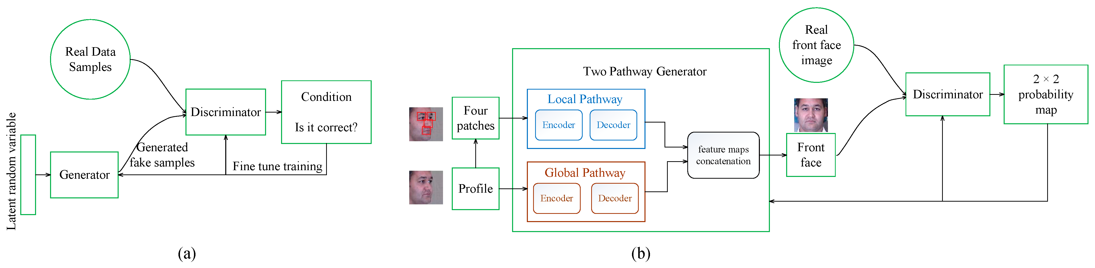
- A posture normalization model, GAN, with two local discriminators (LD-GAN) based on the TP-GAN model, is proposed. The encoder–decoder structure implements a two-pathway generator, global pathway, and local pathway. In order to preserve more local features related to facial expressions in generated frontal faces, the discriminator was improved by adding two local discriminators besides the global discriminator to enhance its adversarial capability against the local pathway encoder. The loss functions are also improved to achieve better effects in network training.
- The effectiveness of this method was verified on three public datasets. The validity of the lightweight FER model was verified on the CK+ and Fer2013 datasets, and the final effect of the combination of the posture normalization model and the FER model was verified on the KDEF dataset. Compared to the methods used in other representative models, this method effectively reduces the number of parameters of our model and has a higher FER rate (92.7%) under the condition of multi-angle deflection.
2. Related Work
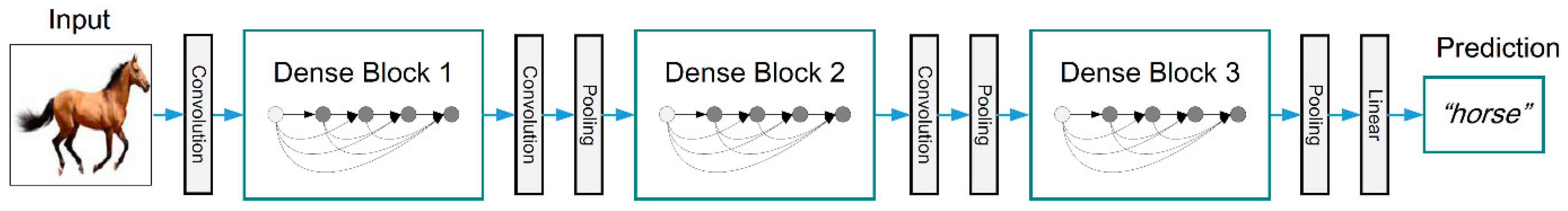
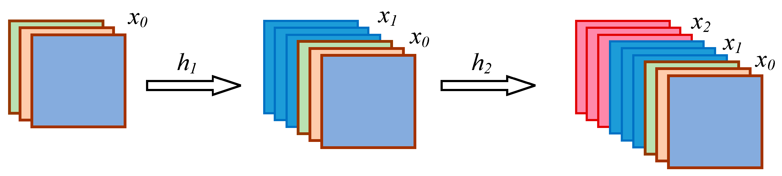
2.1. DenseNet
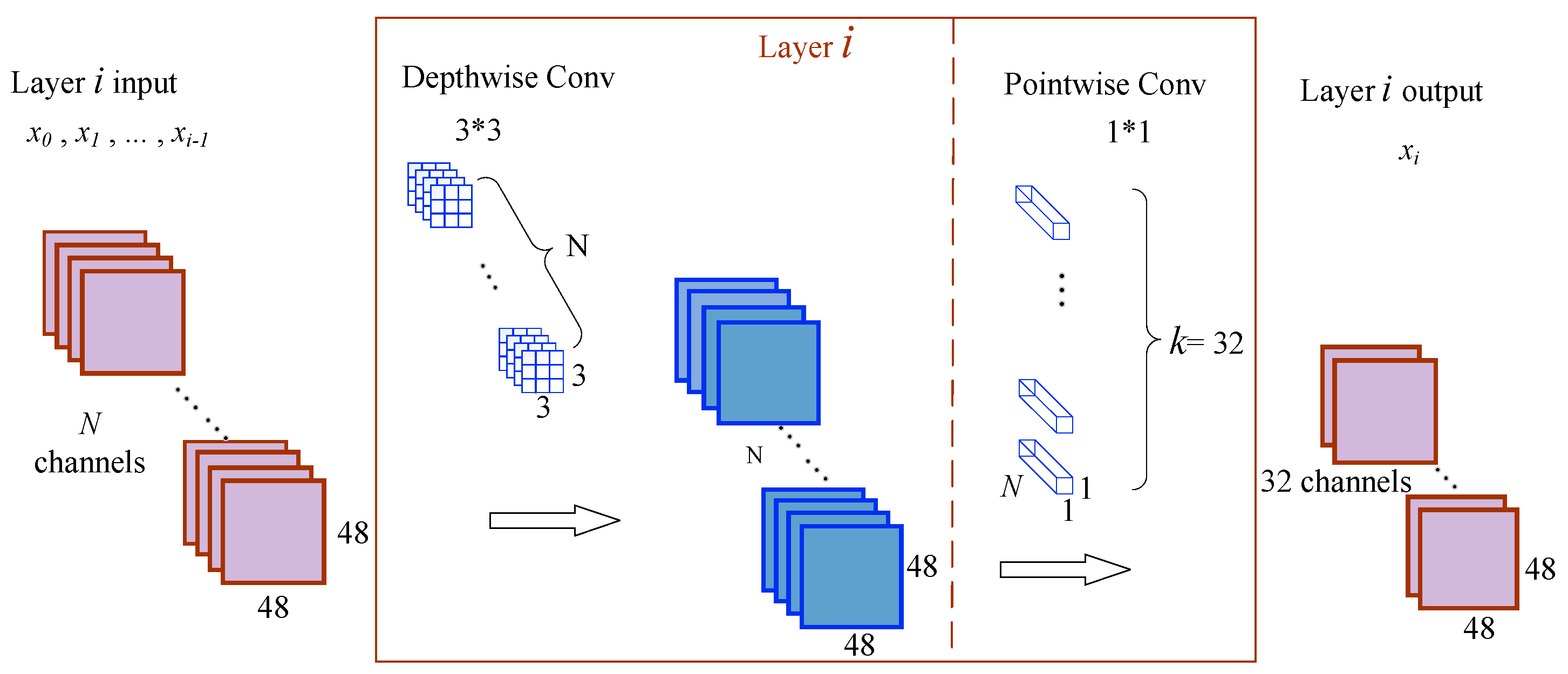
2.2. Depthwise Separable Convolution (DSC)
2.3. GAN and Its Variants
3. Proposed Approach
3.1. Lightweight FER Model: DSC-DenseNet
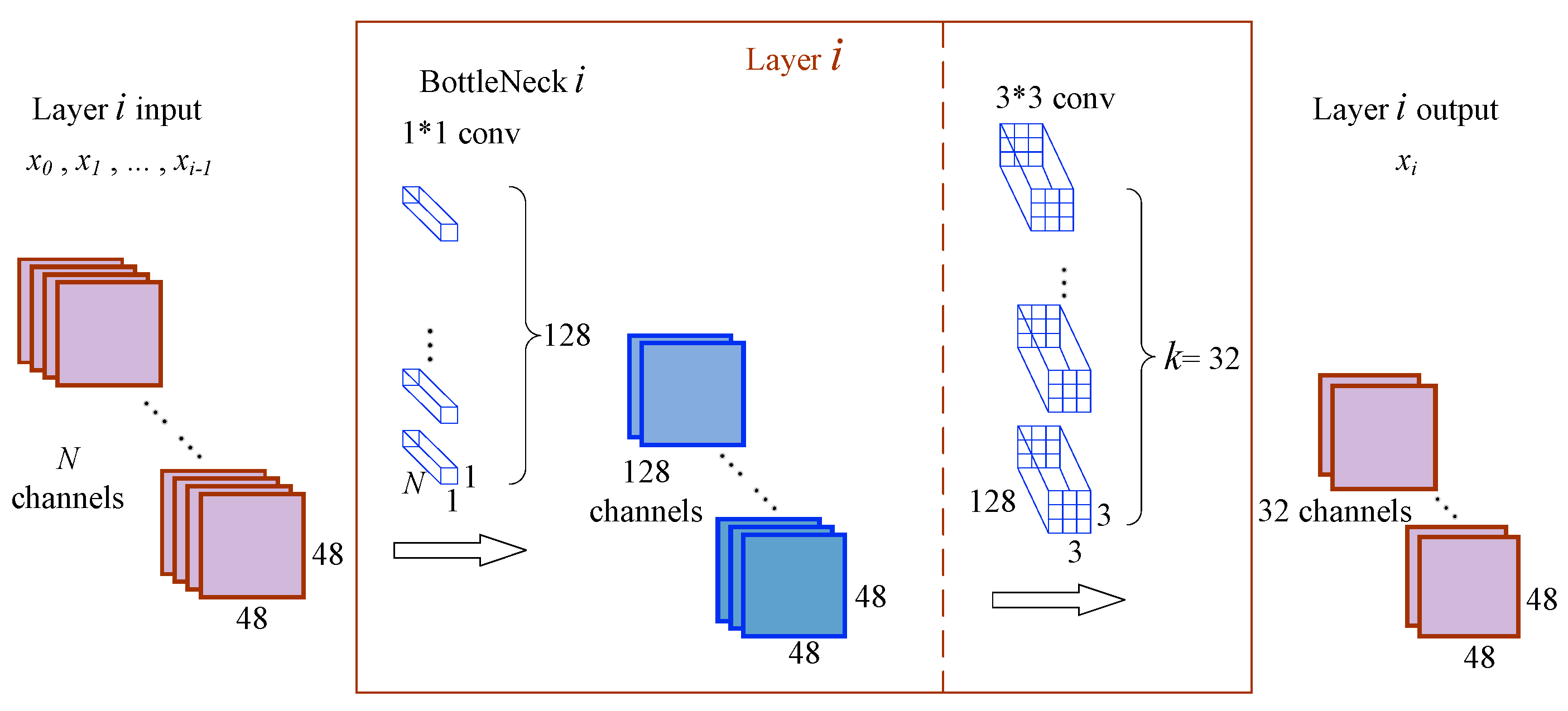
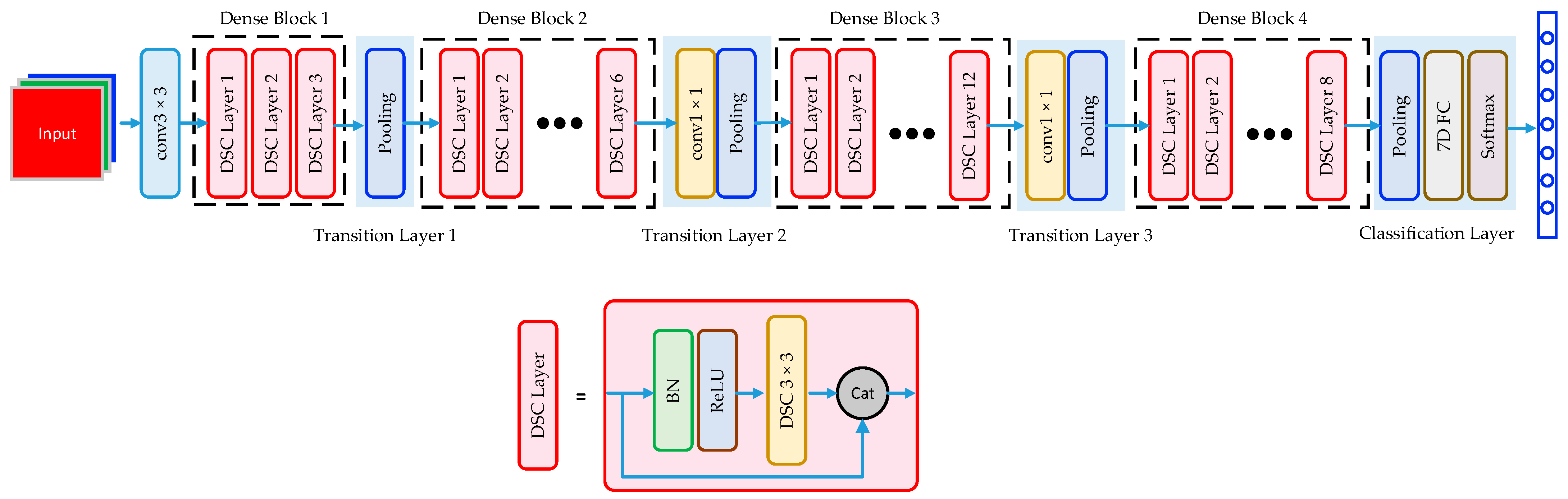
3.1.1. The Framework of Dense Block
3.1.2. The Architecture of DSC-DenseNet
3.2. Frontal Face Normalization Model: GAN with Two Local Discriminators (LD-GAN)
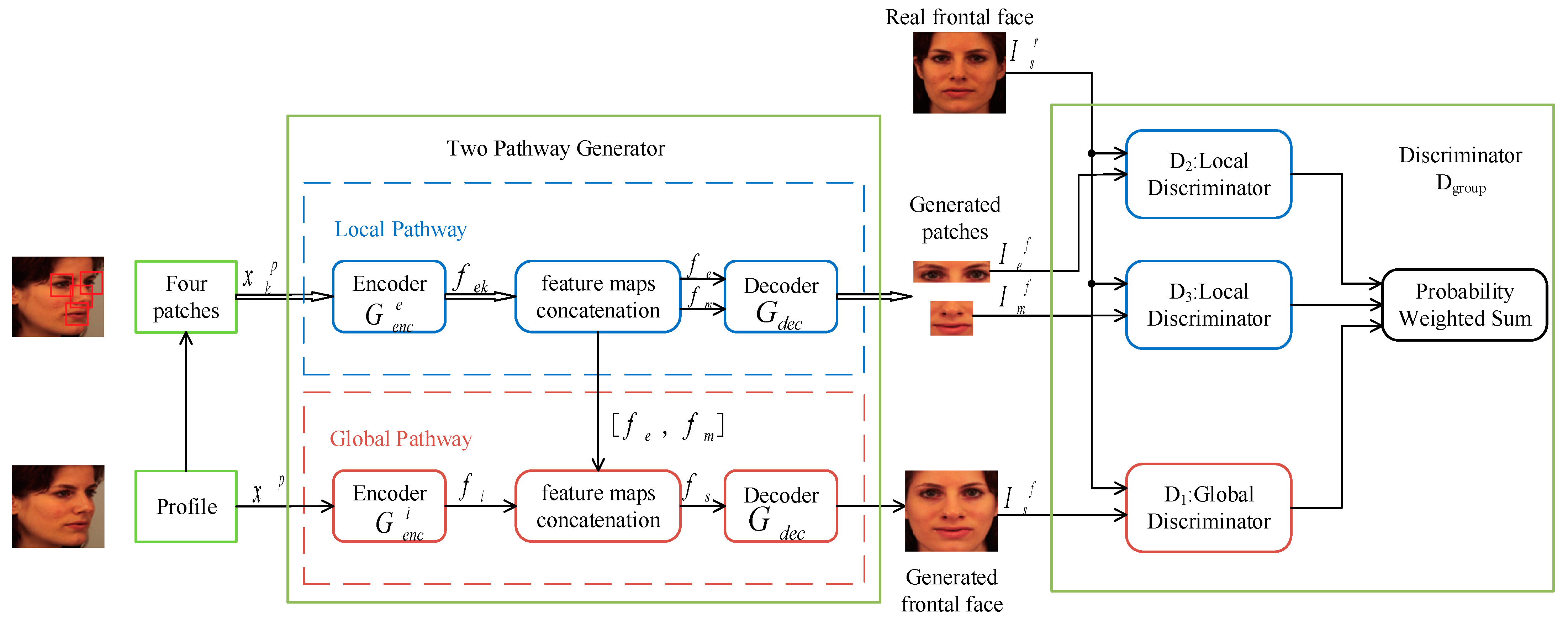
3.2.1. The Framework of LD-GAN
3.2.2. The Architecture of LD-GAN
3.2.3. The Loss Function Improved
4. Experimental Results and Discussions
4.1. Datasets
4.2. Preprocessing
4.3. Experimental Results of DSC-DenseNet
4.3.1. Experiments for Effectiveness of DSC-DenseNet
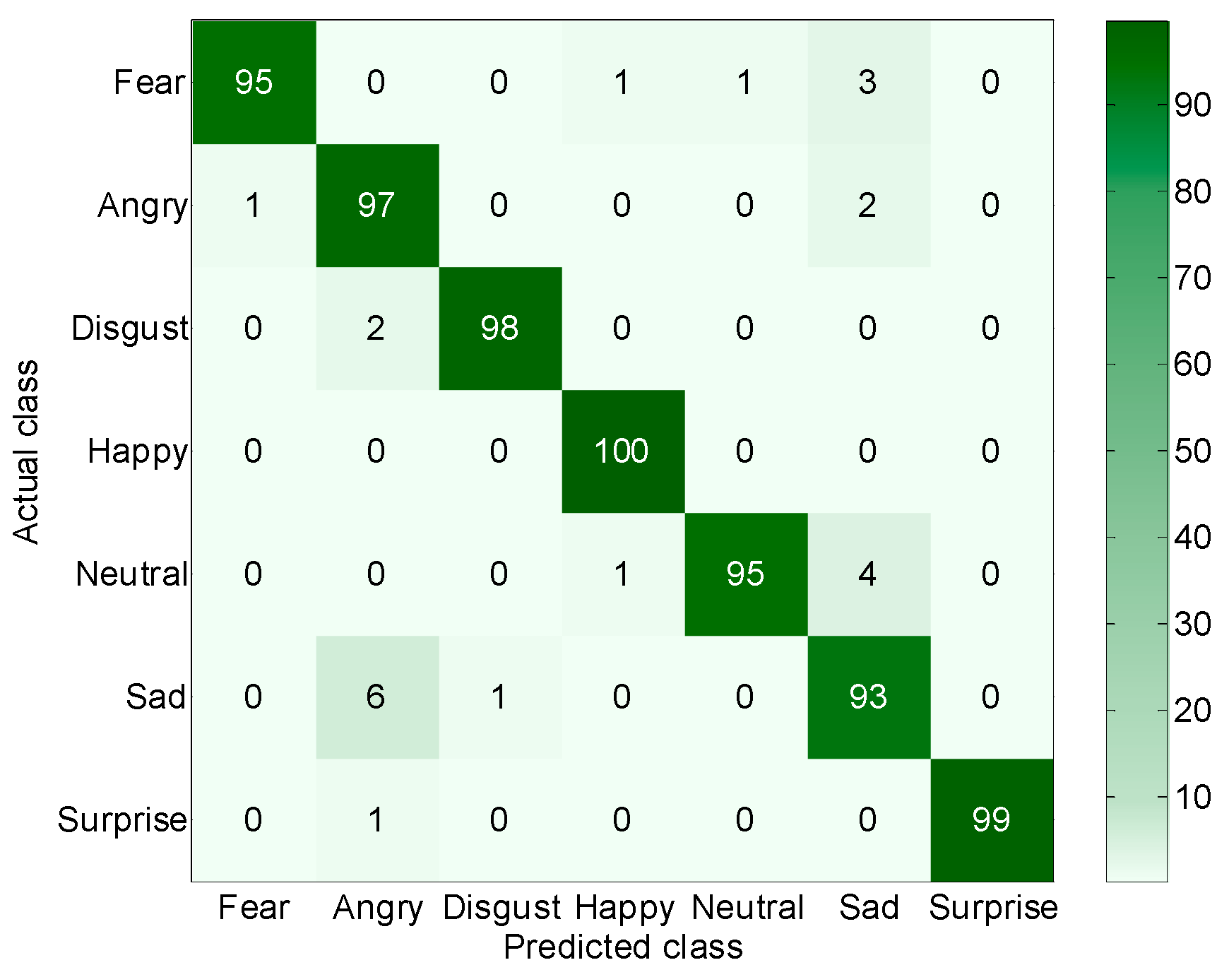
- On the CK+ dataset, the recognition rate of our model was 96.7%. The percentages of recognition for the happiness, surprise, and disgust classes were the highest: 100%, 99%, and 98%, respectively. The reason for the good recognition results for the happiness class was that the features of happiness were more obvious than other emotions and thus it was not easily confused with other features. These results showed the same performance as other existing FER methods. The recognition rate for the sadness class was the lowest—92%—and 6% of sad expressions were misclassified as angry. The reason they were easily confused was that they both more or less involved frowning. Neutral and fear expressions were misclassified as sad in 4% and 3% of cases, respectively.
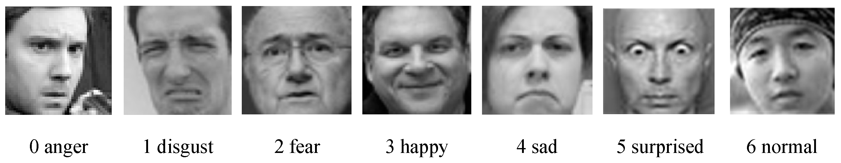
- On the Fer2013 dataset, the recognition rate of our model was 77.3%. The percentages of recognition for the happiness and surprise classes were 93% and 86%, respectively. The recognition rates for the fear and anger classes were the lowest: 62% and 69%, respectively. The main classes that were confused with the fear class were sadness and anger, while the main classes that were confused with the anger class were fear and sadness.
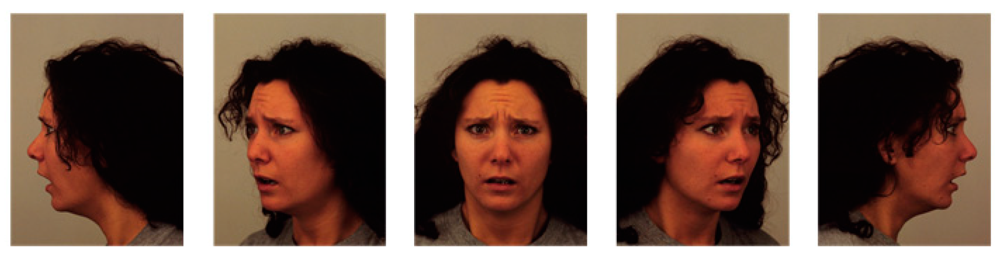
- For CK+, the frontal faces dataset, the recognition rate of our model could meet the practical requirements. For Fer2013, the dataset with profile faces, the recognition rate of our model was significantly reduced. Part of the reason for this was that facial occlusion affected recognition to some extent, although severely occluded samples were removed. Another reason was that there were multi-view images in the dataset, and facial deflection significantly affected the effectiveness of FER. This has also been the consensus among researchers, and it also indicates the necessity of studying facial pose normalization models in this paper.
4.3.2. Comparison of DSC-DenseNet with Other Lightweight Models
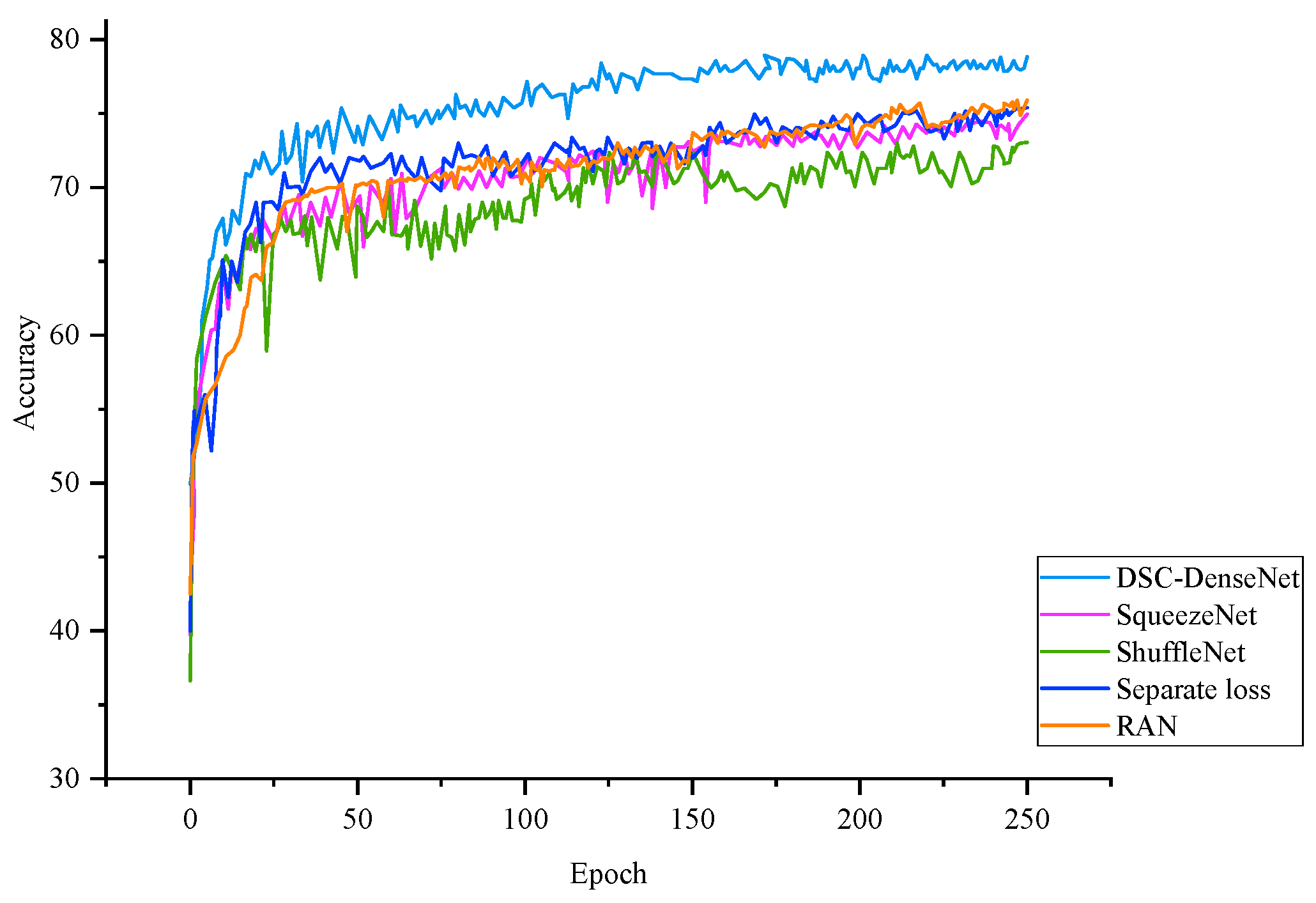
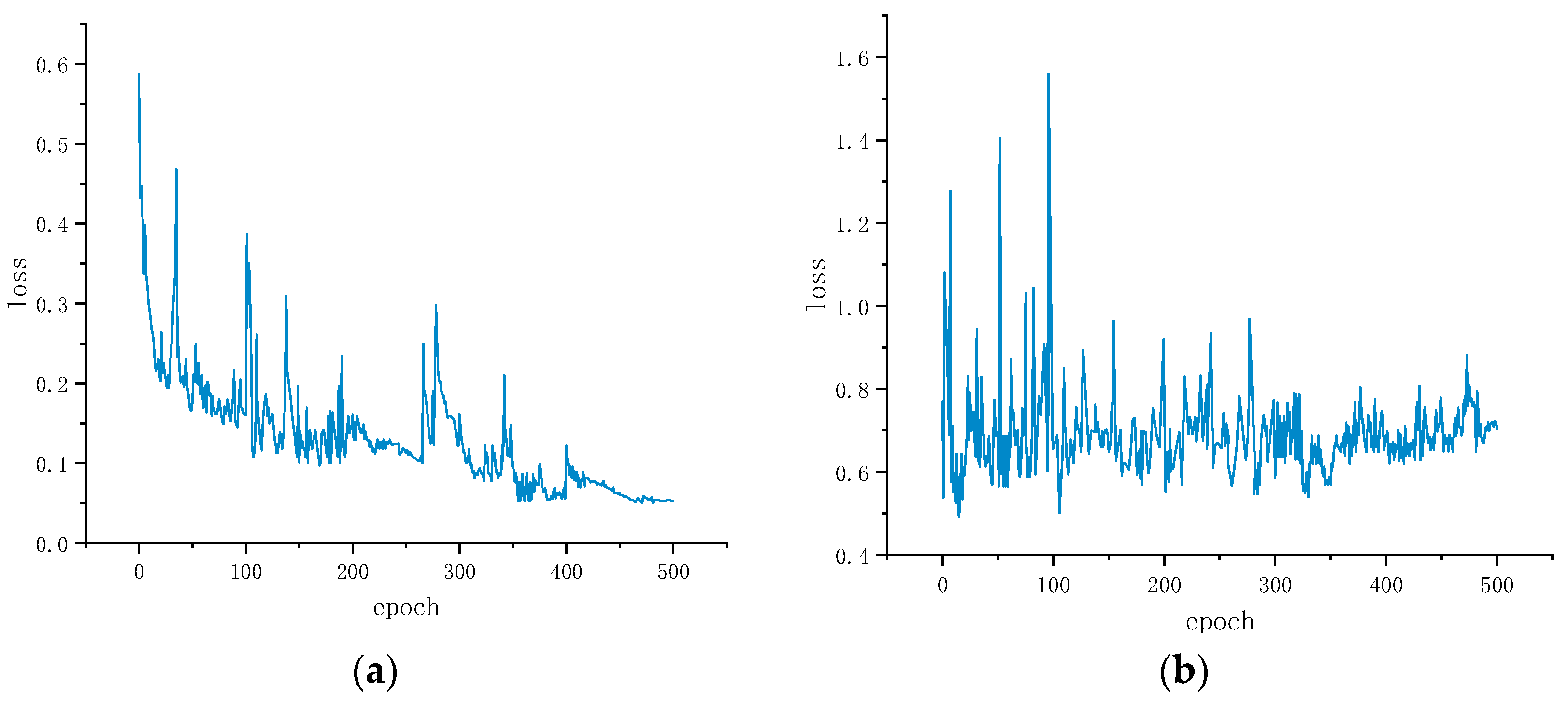
- The FER recognition rate of our model on multi-view faces was 77.3% when the params value was 0.16M. Compared to the models with better accuracy (the lower half of Table 5), such as SqueezeNet and ShuffleNet, our model had higher FLOPs because of its concatenation of feature maps. However, its recognition rate was 2.3% and 4.3% higher than that of SqueezeNet and ShuffleNet, respectively. This could also be seen visually in their learning curves. On the other hand (the upper half of Table 5), it was shown that at the cost of accuracy, speed could be significantly improved. The FLOPs of MobileNetV3 and Light-SE-ResNet were extremely small.
- Our model had a smaller params value to achieve approximate accuracy. Compared to Separate-loss and RAN, the two models with the closest accuracy to ours, the params value of DSC-DenseNet was equal to only about 15% of their params values, and the FLOPs value of DSC-DenseNet was between theirs. Therefore, our model achieved a practical recognition rate, meaning that the lightweight FER model proposed in this paper achieved a balance between the accuracy and performance requirements of the hardware platform.
4.4. Experimental Results of LD-GAN
4.4.1. Training Strategy
4.4.2. Experiments for Effectiveness of LD-GAN
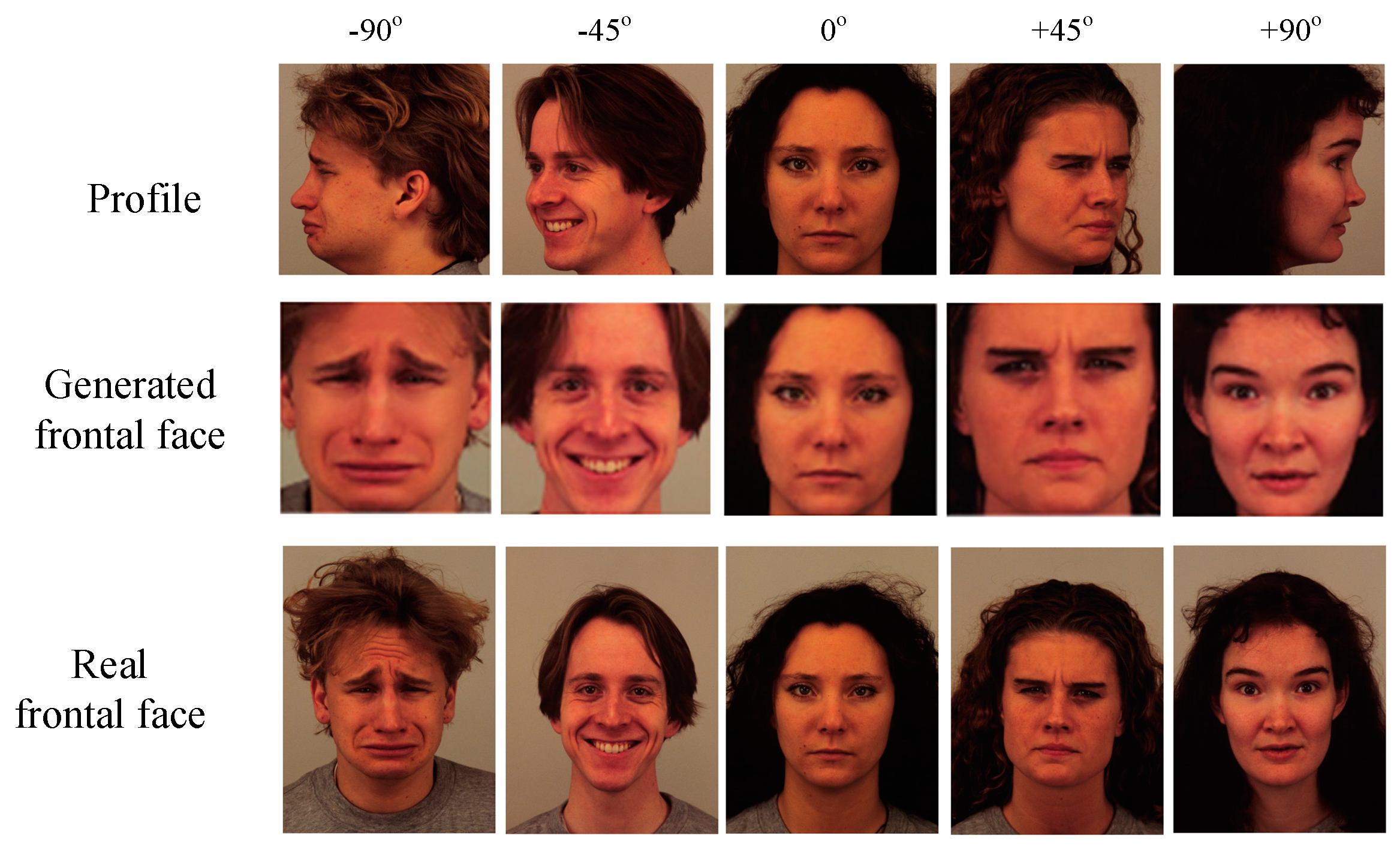
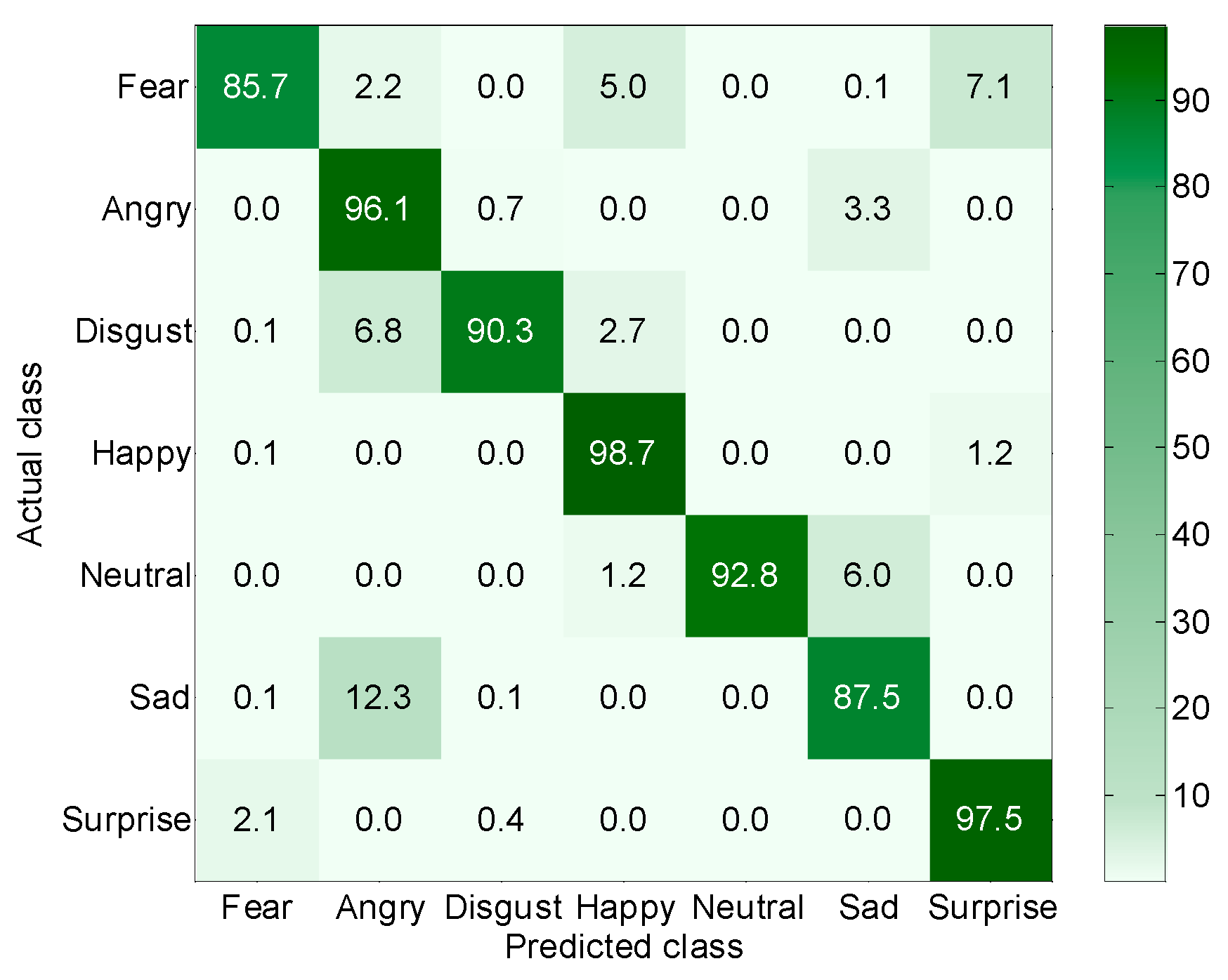
- The recognition rate for happy expressions was the highest: 98.7%. The rates of recognition for the surprise and anger classes were the second highest; these amounted to more than 96%. The recognition rates for the fear and sadness classes were lower: 85.7% and 87.5%, respectively. The mean recognition rate for the seven expressions was 92.7%.
- When compared to the results without pose normalization (Figure 12), the method proposed significantly improved the recognition rate, and could also reduce the misclassification rate between different expressions to a lower level, thus meeting the needs of practical application.
4.4.3. Comparison of Our Model with Others
4.4.4. Ablation Study
5. Conclusions
Author Contributions
Funding
Data Availability Statement
Acknowledgments
Conflicts of Interest
References
- Krizhevsky, A.; Sutskever, I.; Hinton, G.E. ImageNet Classification with Deep Convolutional Neural Networks. Commun. ACM 2017, 60, 84–90. [Google Scholar] [CrossRef]
- Simonyan, K.; Zisserman, A. Very Deep Convolutional Networks for Large-scale Image Recognition. Comput. Sci. 2014, 56, 1–14. [Google Scholar]
- Szegedy, C.; Liu, W.; Jia, Y. Going Deeper with Convolutions. In Proceedings of the IEEE Conference on Computer Vision and Pattern Recognition, Boston, MA, USA, 7–12 June 2015. [Google Scholar]
- He, K.; Zhang, X.; Ren, S.; Sun, J. Deep Residual Learning for Image Recognition. In Proceedings of the IEEE Conference on Computer Vision and Pattern Recognition, Las Vegas, NV, USA, 26 June–1 July 2016. [Google Scholar]
- Girshick, R.; Donahue, J.; Darrell, T.; Malik, J. Rich Feature Hierarchies for Accurate Object Detection and Semantic Segmentation. In Proceedings of the IEEE Conference on Computer Vision and Pattern Recognition, Columbus, OH, USA, 23–28 June 2014. [Google Scholar]
- Ren, S.; He, K.; Girshick, R.; Sun, J. Faster R-CNN: Towards Real-time Object Detection with Region Proposal Networks. IEEE Trans. Pattern Anal. Mach. Intell. 2017, 39, 1137–1149. [Google Scholar] [CrossRef] [PubMed]
- Yao, A.; Cai, D.; Hu, P. HoloNet: Towards Robust Emotion Recognition in the Wild. In Proceedings of the 18th ACM International Conference on Multimodal Interaction, Tokyo, Japan, 12–16 November 2016. [Google Scholar]
- Huang, G.; Liu, Z.; Van Der Maaten, L.; Weinberger, K.Q. Densely Connected Convolutional Networks. In Proceedings of the IEEE Conference on Computer Vision and Pattern Recognition, Honolulu, HI, USA, 21–26 July 2017. [Google Scholar]
- Iandola, F.N.; Han, S.; Moskewicz, M.W.; Ashraf, K.; Dally, W.J.; Keutzer, K. SqueezeNet: AlexNet-level Accuracy with 50× Fewer Parameters and <0.5 MB Model Size. In Proceedings of the International Conference on Learning Representations, Toulon, France, 24–26 April 2017. [Google Scholar]
- Ma, N.; Zhang, X.; Zheng, H.-T.; Sun, J. Shufflenet V2: Practical Guidelines for Efficient CNN Architecture Design. In Proceedings of the European Conference on Computer Vision, Munich, Germany, 8–14 September 2018. [Google Scholar]
- Shen, H.; Meng, Q.; Liu, Y. Facial Expression Recognition by Merging Multilayer Features of Lightweight Convolution Networks. Laser Optoelectron. Prog. 2021, 58, 148–155. [Google Scholar]
- Li, C.; Lu, Y. Facial expression recognition based on depthwise separable convolution. Comput. Eng. Des. 2021, 42, 1448–1454. [Google Scholar]
- Gao, J.; Cai, Y.; He, Z. TP-FER: Facial expression recognition method of tri-path networks based on optimal convolutional neural network. Appl. Res. Comput. 2021, 38, 7. [Google Scholar]
- Liang, H.; Lei, Y. Expression Recognition with Separable Convolution Channel Enhancement Features. Comput. Eng. Appl. 2022, 58, 184–192. [Google Scholar]
- Zhang, P.; Kong, W.; Teng, J. Facial Expression Recognition Based on Multi-scale Feature Attention Mechanism. Comput. Eng. Appl. 2022, 58, 182–189. [Google Scholar]
- Han, Z. Facial Expression Recognition under Various Facial Postures. Master’s Thesis, Soochow University, Suzhou, China, 2020. [Google Scholar]
- Goodfellow, I.; Pouget-Abadie, J.; Mirza, M.; Xu, B.; Warde-Farley, D.; Ozair, S.; Courville, A.; Bengio, Y. Generative Adversarial Nets. In Proceedings of the Neural Information Processing Systems, Montreal, QC, Canada, 8–11 December 2014. [Google Scholar]
- Chollet, F. Xception: Deep learning with depthwise separable convolutions. In Proceedings of the IEEE Conference on Computer Vision and Pattern Recognition, Honolulu, HI, USA, 21–26 July 2017. [Google Scholar]
- Howard, A.G.; Zhu, M.; Chen, B.; Kalenichenko, D.; Wang, W.; Weyand, T.; Andreetto, M.; Adam, H. Mobilenets: Efficient convolutional neural networks for mobile vision applications. In Proceedings of the IEEE Conference on Computer Vision and Pattern Recognition, Honolulu, HI, USA, 21–26 July 2017. [Google Scholar]
- Generative Adversarial Network (GAN). Available online: https://www.geeksforgeeks.org/generative-adversarial-network-gan/ (accessed on 31 March 2023).
- Huang, R.; Zhang, S.; Li, T.; He, R. Beyond Face Rotation: Global and Local Perception GAN for Photorealistic and Identity Preserving Frontal View Synthesis. In Proceedings of the IEEE International Conference on Computer Vision, Venice, Italy, 22–29 October 2017. [Google Scholar]
- Yin, X.; Yu, X.; Sohn, K.; Liu, X.; Chandraker, M. Towards Large-Pose Face Frontalization in the Wild. In Proceedings of the IEEE International Conference on Computer Vision, Venice, Italy, 22–29 October 2017. [Google Scholar]
- Tran, L.; Yin, X.; Liu, X. Disentangled Representation Learning GAN for Pose-invariant Face Recognition. In Proceedings of the IEEE Conference on Computer Vision and Pattern Recognition, Honolulu, HI, USA, 21–26 July 2017. [Google Scholar]
- Hu, Y.; Wu, X.; Yu, B.; He, R.; Sun, Z. Pose-guided Photorealistic Face Rotation. In Proceedings of the IEEE Conference on Computer Vision and Pattern Recognition, Salt Lake City, UT, USA, 18–22 June 2018. [Google Scholar]
- Hardy, C.; Le Merrer, E.; Sericola, B. MD-GAN: Multi-Discriminator Generative Adversarial Networks for Distributed Datasets. In Proceedings of the IEEE International Parallel and Distributed Processing Symposium, Rio de Janeiro, Brazil, 20–24 May 2019. [Google Scholar]
- Lin, H.; Ma, H.; Gong, W.; Wang, C. Non-frontal Face Recognition Method with a Side-face-correction Generative Adversarial Networks. In Proceedings of the 3rd International Conference on Computer Vision, Image and Deep Learning, Changchun, China, 20–22 May 2022. [Google Scholar]
- Iizuka, S.; Simo-serra, E.; Ishikawa, H. Globally ang Locally Consistent Image Completion. ACM Trans. Graph. 2017, 36, 1–14. [Google Scholar] [CrossRef]
- Sharma, A.K.; Foroosh, H. Slim-CNN: A Light-Weight CNN for Face Attribute Prediction. In Proceedings of the IEEE International Conference on Automatic Face & Gesture Recognition, Buenos Aires, Argentina, 18–22 May 2020. [Google Scholar]
- Extended Cohn-Kanade Dataset. Available online: http://www.pitt.edu/~emotion/ck-spread.htm (accessed on 19 April 2023).
- Kaggle FER Challenge Dataset. Available online: https://www.kaggle.com/c/challenges-in-representation-learning-facial-expression-recognition-challenge/overview (accessed on 19 April 2023).
- Karolinska Directed Emotional Faces. Available online: http://www.emotionlab.se/kdef (accessed on 19 April 2023).
- Zhang, K.; Zhang, Z.; Li, Z.; Qiao, Y. Joint Face Detection and Alignment Using Multitask Cascaded Convolutional Networks. IEEE Signal Process. Lett. 2017, 23, 1499–1503. [Google Scholar] [CrossRef]
- Xia, H.; Li, C. Face Recognition and Application of Film and Television Actors Based on Dlib. In Proceedings of the International Congress on Image and Signal Processing, Biomedical Engineering and Informatics, Suzhou, China, 19–21 October 2019. [Google Scholar]
- Howard, A.; Sandler, M.; Chu, G.; Chen, L.C.; Chen, B.; Tan, M.; Wang, W.; Zhu, Y.; Pang, R.; Vasudevan, V.; et al. Searching for MobileNetV3. In Proceedings of the IEEE International Conference on Computer Vision, Seoul, Republic of Korea, 27 October–2 November 2019. [Google Scholar]
- Xie, Y. Research and Application of Facial Expression Recognition Method Based on Deep Learning Architecture. Master’s Thesis, Wuhan Institute of Technology, Wuhan, China, 25 May 2022. [Google Scholar]
- Yang, H. Facial Expression Recognition Method Based on Lightweight Convolutional Neural Network. Master’s Thesis, Beijing University of Civil Engineering and Architecture, Beijing, China, 30 May 2020. [Google Scholar]
- Li, Y.; Lu, Y.; Li, J.; Lu, G. Separate Loss for Basic and Compound Facial Expression Recognition in the Wild. In Proceedings of the Eleventh Asian Conference on Machine Learning, WINC AICHI, Nagoya, Japan, 17–19 November 2019. [Google Scholar]
- Wang, K.; Peng, X.; Yang, J.; Meng, D.; Qiao, Y. Region Attention Networks for Pose and Occlusion Robust Facial Expression Recognition. IEEE Trans Image Process. 2020, 29, 4057–4069. [Google Scholar] [CrossRef] [PubMed]


| Layers | Operator | Output Size | Output Channels |
|---|---|---|---|
| Convolution | 3 × 3 conv, stride 1 | 48 × 48 | 32 |
| Dense Block1 | 3 × 3 DSC × 3 layers | 48 × 48 | 32 + 32 × 3 = 128 |
| Transition Layer1 | 2 × 2 average pool, stride 2 | 24 × 24 | 128 |
| Dense Block2 | 3 × 3 DSC × 6 layers | 24 × 24 | 128 + 32 × 6 = 320 |
| Transition Layer2 | 1 × 1 × 128 conv | 24 × 24 | 128 |
| 2 × 2 average pool, stride 2 | 12 × 12 | 128 | |
| Dense Block3 | 3 × 3 DSC × 12 layers | 12 × 12 | 128 + 32 × 12 = 512 |
| Transition Layer3 | 1 × 1 × 256 conv | 12 × 12 | 256 |
| 2 × 2 average pool, stride 2 | 6 × 6 | 256 | |
| Dense Block4 | 3 × 3 DSC × 8 layers | 6 × 6 | 256 + 32 × 8 = 512 |
| Classification Layer | 6 × 6 global average pool | 1 × 1 | - |
| 7D fully-connected, softmax | - | - |
| Layer | Kernel/Stride | Output |
|---|---|---|
| Conv0 | 7 × 7/1 | 128 × 128 × 64 |
| Conv1 | 5 × 5/2 | 64 × 64 × 64 |
| Conv2 | 3 × 3/2 | 32 × 32 × 128 |
| Conv3 | 3 × 3/2 | 16 × 16 × 256 |
| Conv4 | 3 × 3/2 | 8 × 8 × 512 |
| fc1 | - | 512 |
| fc2 | - | 256 |
| Layers | Kernel | Output |
|---|---|---|
| fc reshape | - | 8 × 8 × 64 |
| Deconv0 | 3 × 3 | 16 × 16 × 64 |
| Deconv1 | 3 × 3 | 32 × 32 × 32 |
| Deconv2 | 3 × 3 | 64 × 64 × 16 |
| Deconv3 | 3 × 3 | 128 × 128 × 16 |
| Deconv4 | 3 × 3 | 128 × 128 × 3 |
| Layer | Kernel/Stride | Output |
|---|---|---|
| Conv0 | 4 × 4/2 | 64 × 64 × 64 |
| Conv1 | 4 × 4/2 | 32 × 32 × 128 |
| Conv2 | 4 × 4/2 | 16 × 16 × 256 |
| Conv3 | 4 × 4/2 | 8 × 8 × 512 |
| Conv4 | 4 × 4/2 | 4 × 4 × 1024 |
| Conv5 | 4 × 4/1 | 1 × 1 × 1024 |
| Lightweight Model | Params (Million) | FLOPs (Billion) | Recognition Rate (95%CI) |
|---|---|---|---|
| MobileNetV3 (Large) [34] | 4.2 | 0.02 | 63.9% ± 1.49% |
| Light-SE-ResNet [35] | 5.1 | 0.06 | 67.4% ± 1.45% |
| ResNet18 [4] | 11.2 | 0.09 | 69.3% ± 1.43% |
| ResNet50 | 23.5 | 0.21 | 70.1% ± 1.42% |
| ShuffleNet [10] | 1.25 | 0.04 | 73.0% ± 1.38% |
| PGC-DenseNet [36] | 0.26 | 0.12 | 73.3% ± 1.37% |
| SqueezeNet [9] | 0.47 | 0.02 | 75.0% ± 1.34% |
| Separate-loss [37] | 1.1 | 0.18 | 75.4% ± 1.33% |
| RAN [38] | 1.2 | 0.14 | 76.0% ± 1.32% |
| DSC-DenseNet (Ours) | 0.16 | 0.16 | 77.3% ± 1.30% |
Disclaimer/Publisher’s Note: The statements, opinions and data contained in all publications are solely those of the individual author(s) and contributor(s) and not of MDPI and/or the editor(s). MDPI and/or the editor(s) disclaim responsibility for any injury to people or property resulting from any ideas, methods, instructions or products referred to in the content. |
© 2023 by the authors. Licensee MDPI, Basel, Switzerland. This article is an open access article distributed under the terms and conditions of the Creative Commons Attribution (CC BY) license (https://creativecommons.org/licenses/by/4.0/).
Share and Cite
Dong, J.; Zhang, Y.; Fan, L. A Multi-View Face Expression Recognition Method Based on DenseNet and GAN. Electronics 2023, 12, 2527. https://doi.org/10.3390/electronics12112527
Dong J, Zhang Y, Fan L. A Multi-View Face Expression Recognition Method Based on DenseNet and GAN. Electronics. 2023; 12(11):2527. https://doi.org/10.3390/electronics12112527
Chicago/Turabian StyleDong, Jingwei, Yushun Zhang, and Lingye Fan. 2023. "A Multi-View Face Expression Recognition Method Based on DenseNet and GAN" Electronics 12, no. 11: 2527. https://doi.org/10.3390/electronics12112527
APA StyleDong, J., Zhang, Y., & Fan, L. (2023). A Multi-View Face Expression Recognition Method Based on DenseNet and GAN. Electronics, 12(11), 2527. https://doi.org/10.3390/electronics12112527