Adaptive NN Control of Electro-Hydraulic System with Full State Constraints

Abstract

This paper presents an adaptive neural network (NN) control approach for an electro-hydraulic system. The friction and internal leakage are nonlinear uncertainties, and the states in the considered electro-hydraulic system are fully constrained. In the control design, the NNs are utilized to approximate the nonlinear uncertainties. Then, by constructing barrier Lyapunov functions and based on the adaptive backstepping control design technique, a novel adaptive NN control scheme is formulated. It has been proven that the developed adaptive NN control scheme can sustain the controlled electro-hydraulic system to be stable and make the system output track the desired reference signal. Furthermore, the system states do not surpass the given bounds. The computer simulation results verify the effectiveness of the proposed controller.

1. Introduction

Electro-hydraulic systems are widely employed in sundry industrial applications such as robotic manipulators, active suspensions, precision machine tools, and aerospace systems. They provide many advantages over electric motors, including a high force to weight ratio, fast response time, and compact size. With the increasing applications of hydraulic mechanisms, the issue of stabilizing electro-hydraulic systems has attracted tremendous attention in recent years. To handle this issue, many control methods were developed. For instance, [1] presented a nonlinear adaptive robust control method for a single-rod electro-hydraulic actuator with unknown nonlinear parameters. By employing the control method and constructing a novel-type Lyapunov function, [2] developed an adaptive sliding mode control controller. In [3], an active fault-tolerant control (FTC) system is proposed against the valve faults of an independent metering valve. Backstepping control [4] was also widely used in EHS in handling mismatched disturbances. In [5], an output feedback nonlinear control is proposed for EHS, in which an extended state observer (ESO) and a nonlinear robust controller are synthesized via backstepping. In order to solve the uncertain nonlinearity and parameter uncertainty in hydraulic systems simultaneously, a nonlinear adaptive robust control method is presented in [6]. Further, a robust integral of the sign of the error controller and an adaptive controller is synthesized via the backstepping method for motion control of a hydraulic rotary actuator in [7], which theoretically guaranteed asymptotic tracking performance in the presence of various uncertainties. In [8], a practical nonlinear adaptive repetitive controller is proposed for motion control of hydraulic servo-mechanisms to learn and compensate for the periodic modeling uncertainties.

It should be mentioned that since the tolerance of the hydraulic rotary actuator is finite, the load pressure should be limited to a feasible boundary, and the rate limit of the hydraulic rotary actuator’s response cannot be that large. To ensure that all the state variables are not violating their constraints and the normal operation of the controlled system, it is important to investigate the issue of state constraints in the control problem of EHS. In [9], a high-gain disturbance observer (HGDOB)-based backstepping controller was proposed for electro-hydraulic systems with position tracking error constraints. To suppress the violation of tracking error constraints, a barrier Lyapunov function-based dynamic surface control method was proposed for the position tracking control of the ammunition manipulator in [10].

Note that the control schemes mentioned above all require precise structural information of the considered hydraulic system. Especially, the frictions and internal leakage are both required to be known. Therefore, they do not effectively control the hydraulic systems with nonlinear uncertainties. Fuzzy systems [11] and neural networks [12,13,14,15] have good approximation performance, and thus they are frequently utilized to deal with uncertainties in nonlinear systems. In [16], the authors integrated fuzzy learning mechanisms into the modeling of EHS and proposed a kind of fuzzy PI controller. In [17], a neural adaptive control was developed for single-rod EHS to improve the dynamic tracking performance of the cylinder position under lumped uncertainties. Although these control methods improved the position tracking performance without precise knowledge of the EHS, they did not consider the control problem of EHS with state constraints.

Inspired by the above observations, this paper investigates the adaptive tracking control problem for an electro-hydraulic system with nonlinear uncertainties and full state constraints. By utilizing neural networks to model the nonlinear uncertainties, and constructing the barrier Lyapunov functions, an adaptive NN control approach is developed in the framework of adaptive backstepping control design. The main advantages of the proposed adaptive NN control scheme are as follows: it can ensure the controlled electro-hydraulic system is stable and make the system output track the desired reference signal. Furthermore, the system states are confined within the given compact sets and do not surpass their bounds. Note that the previous adaptive NN controller [17] also addressed the control problem for electro-hydraulic systems with lumped uncertainties by neural network approximation. However, detailed information such as the frictions and internal leakage was still required, the neural networks were merely utilized to approximate the lumped uncertainties composed of parameter uncertainties and the external disturbance. Furthermore, it did not consider the control problem for electro-hydraulic systems with state constraints. On the other hand, although [9] studied the control problem for electro-hydraulic systems with state constraints, it required the nonlinear dynamics of the electro-hydraulic system to be exactly known.

2. Problem Formulation and Preliminaries

2.1. Hydraulic System Model

The hydraulic system [5] under study is illustrated in Figure 1. On the left in Figure 1, an inertia load is driven by a servo valve-controlled hydraulic rotary actuator, whose schematic structure is presented on the right in Figure 1. The motion dynamics of the inertia load can be described by

$$J\ddot{y}=P_L{D}_m-F(y,\dot{y})+f(t)$$

(1)

where $J$ and $y$ represent the moment of inertia and the angular displacement of the load, respectively; $P_L=P_1-P_2$ is the load pressure of the hydraulic actuator, $P_1$ and $P_2$ are the pressures inside the two chambers of the actuator; $D_m$ is the radian displacement of the actuator; $F$ represents any continuous differentiable friction model, and $f$ represents other disturbances. The load pressure dynamics can be written as

$$\frac{V_t}{4{\beta }_e}{\dot{P}}_L=-D_m\dot{y}-Q_t(P_L)+Q(t)+Q_L$$

(2)

where $V_t$ is the total control volume of the actuator; ${\beta }_e$ is the effective oil bulk modulus; $Q_t(P_L)$ is the total internal leakage of the actuator due to pressure; $Q(t)$ is the time-varying disturbances and external leakage; $Q_L=\left(Q_1+Q_2\right)/2$ is the load flow, $Q_1$ is the supplied flow rate to the forward chamber, and $Q_2$ is the return flow rate of the return chamber. $Q_L$ is related to the spool valve displacement of the servo valve, i.e., $x_V$, by

$$Q_L=k_q{x}_v\sqrt{P_s-sign(x_v)P_L}$$

(3)

where $k_q=C_d\omega \sqrt{1/\rho }$ is the flow gain, and $sign(x_v)$ is given as

$$sign(x_v)=\left\{\begin{array}{l}1,if x_v\ge 0\\ -1, if x_v<0\end{array}\right.$$

(4)

where $C_d$ is the discharge coefficient; $\omega$ is the spool valve area gradient; $\rho$ is the density of oil; $P_s$ is the supply pressure of the fluid with respect to the return pressure $P_r$.

Although the model of servo valve dynamics is actually nonlinear, which has been considered by some researchers [6], only minimal performance improvement can be achieved for motion tracking, and additional sensors are required to obtain the spool position. Therefore, many studies neglect servo valve dynamics. So, in this paper, the relationship between the control applied to the servo valve and the spool position is defined as $x_v=k_{i}u$, i.e., the control applied to the servo valve is directly proportional to the spool position, where $x_v$ is the spool position and $u$ is the control input voltage, since a high-response servo valve is used here. Thus, (3) can be transformed to

$$Q_L=k_{t}u\sqrt{P_s-sign(u)P_L}$$

(5)

Since only variables $y$, $\dot{y}$ and $P_L$ are necessary to be controlled for hydraulic motion systems, so defining the state variables as $X={[x_1,x_2,x_3]}^T={[y,\dot{y},D_m{P}_L/J]}^T$ is sufficient for controller design. Then, the considered electro-hydraulic system can be expressed in a state-space form as

$$\left\{\begin{array}{l}{\dot{x}}_1=x_2\\ {\dot{x}}_2=x_3+{\varphi }_1(x_2)+d_1(t)\\ {\dot{x}}_3=g(x_3,u)u+{\varphi }_2(x_2,x_3)+d_2(t)\end{array}\right.$$

(6)

where, ${\varphi }_1(x_2)=-F(x_2)/J,d_1(t)=f(t)/J$, and

$${\varphi }_2(x_2,x_3)=-\frac{4D_m^2{\beta }_e}{J{V}_t}{x}_2-\frac{4{\beta }_e}{V_t}{Q}_t(x_3)$$

(7)

$$d_2(t)=4{\beta }_e{D}_{m}Q(t)/(V_{t}J)$$

(8)

$$g(x_3,u)=\frac{4D_m{\beta }_e{k}_t}{J{V}_t}\sqrt{P_S-sign(u)J{x}_3/D_m}$$

(9)

Remark 1.

It should be pointed out that the nonlinear friction models and the nonlinear internal leakage models used in this study are not considered by the previous studies. The nonlinear friction $F\left(x_2\right)$ and the nonlinear internal leakage $Q_t(x_3)$ are both considered nonlinear uncertainties. Thus, ${\varphi }_1(x_2)$ and ${\varphi }_2(x_2,x_3)$ in (6) are all unknown nonlinear functions.

Assumption 1

[18]. There exist positive constants $A_0$, $A_1$ and $A_2$ such that the given reference $y_d$ and its derivatives satisfy $\left|y_d\right|\le A_0<k_{c1}$ and $\left|y_d^{(i)}\right|\le A_i\left(i=1,2\right)$.

Assumption 2.

There exist positive constants $k_{ci}$ such that the system states satisfy the restrictions: $\left|x_i\right|<k_{ci}, i=1,2,3$.

Control Objective. The objective of this study is to propose an adaptive NN control scheme. The proposed adaptive NN control scheme can make the controlled electro-hydraulic system stable and $y$ track the desired trajectory $y_d$. Moreover, the system states do not violate their bounds.

2.2. Radial Basis Function Neural Networks

A radial basis function neural network (RBFNN) [19] can be expressed as

$$\widehat{f}(X|W)=W^{T}S(X)$$

(10)

where $X\in R^m$ is the input vector, $W\in R^r$ is the weight vector with neurons number $r$. $S(X)={\left[s_1(X),\dots ,s_r(X)\right]}^T$, where $s_i(X)$ is a Gaussian-type basis function, which can be selected as

$$s_i(X)=\exp \left\{-\frac{{\left(X-o_i\right)}^T\left(X-o_i\right)}{{\rho }_i^2}\right\}$$

(11)

where ${\rho }_i$ and $o_i\in R^m$ are the width of the Gaussian function and the center vector, respectively.

It is well known that an RBFNN can be used to approximate any a continuous function $F(X)$ as [20]

$$F(X)=W^{*}{}^{T}S(X)+\epsilon (X)$$

(12)

where $W^{*}$ is the ideal constant vector and $\epsilon (X)$ is the approximation error.

3. The Controller Design and Stability Analysis

3.1. Controller Design

Make the following variable transformation:

$$\left\{\begin{array}{c}{z}_1=x_1-y_d\\ z_2=x_2-{\alpha }_1\\ z_3=x_3-{\alpha }_2\end{array}\right.$$

(13)

where $y_d$ represents the desired trajectory, ${\alpha }_1$ and ${\alpha }_2$ represent the virtual control variables to be designed later.

Based on the above variable transformation, we will give the detailed three-step backstepping control [21] design procedures for the electro-hydraulic system (6).

Step 1: Noting (6), the time derivative of tracking error $z_1$ is

$${\dot{z}}_1=x_2-{\dot{y}}_d$$

(14)

Construct a barrier Lyapunov function candidate as

$$V_1=\frac{1}{2}\ln \frac{k_{b1}^2}{k_{b1}^2-z_1{}^2}$$

(15)

where $k_{b1}$ is a positive constant. It is obvious that in ${\Omega }_{z_1} :=\left\{z_1:\left|z_1\right|<k_{b1}\right\}$, $V_1$ is a continuous differentiable. Then, the time derivative of $V_1$ can be derived as follows

$$\begin{array}{l}{\dot{V}}_1=\frac{z_1{\dot{z}}_1}{k_{b1}^2-z_1^2}\\ =\frac{z_1}{k_{b1}^2-z_1^2}\left(x_2-{\dot{y}}_d\right)\\ =\frac{z_1}{k_{b1}^2-z_1^2}\left(z_2+{\alpha }_1-{\dot{y}}_d\right)\end{array}$$

(16)

Design the virtual controller ${\alpha }_1$ as

$${\alpha }_1={\dot{y}}_d-c_1{z}_1$$

(17)

where $c_1$ is a positive design parameter.

Step 2: From (6), the derivative of $z_2=x_2-{\alpha }_1$ with respect to time is given by

$$\begin{array}{l}{\dot{z}}_2=x_3+{\varphi }_1(x_2)+d_1(t)-{\dot{\alpha }}_1\\ =z_3+{\alpha }_2+{\varphi }_1(x_2)+d_1(t)-{\dot{\alpha }}_1\end{array}$$

(18)

Based on the neural approximation, we can assume that

$${\varphi }_1(x_2)=W_1^{*}{}^T{S}_1(x_2)+{\epsilon }_1(x_2)$$

(19)

where $W_1^{*}$ denotes the ideal weight vector, $S_1(x_2)={\left[s_1(x_2),\dots ,s_{r_1}(x_2)\right]}^T$ is the radial basis vector with Gaussian function $s_j(x_2), j=1,2,\dots ,r_1$. ${\epsilon }_1$ is the approximation error satisfying $\left|{\epsilon }_1\right|\le {\overline{\epsilon }}_1$ with the constant ${\overline{\epsilon }}_1>0$. Then (17) becomes

$${\dot{z}}_2=z_3+{\alpha }_2+W_1^{*}{}^T{S}_1(x_2)+{\epsilon }_1(x_2)+d_1(t)-{\dot{\alpha }}_1$$

(20)

Construct a barrier Lyapunov function candidate as

$$V_2=\frac{1}{2}\ln \frac{k_{b2}^2}{k_{b2}^2(t)-z_2{}^2}+\frac{1}{2}{\sigma }_1{\tilde{W}}_1^T{\tilde{W}}_1$$

(21)

where ${\sigma }_1$ is a positive design parameter, and $k_{b2}$ is a positive constant. In ${\Omega }_{z_2} :=\left\{z_2:\left|z_2\right|<k_{b2}\right\}$, $V_2$ is a continuous differentiable. Then the time derivative of $V_2$ can be derived as

$${\dot{V}}_2=\frac{z_2{\dot{z}}_2}{k_{b2}^2-z_2^2}+{\sigma }_1{\dot{\tilde{W}}}_1^T{\tilde{W}}_1$$

(22)

From (20) and (22), the following equation can be obtained

$${\dot{V}}_2=\frac{z_2}{k_{b2}^2-z_2^2}(z_3+{\alpha }_2+W_1^{*}{}^T{S}_1(x_2)+{\epsilon }_1(Z_1)+d_1(t)-{\dot{\alpha }}_1)+{\sigma }_1{\dot{\widehat{W}}}_1^T{\tilde{W}}_1$$

(23)

The virtual controller ${\alpha }_2$ and the adaptive law of ${\widehat{W}}_1$ are designed as

$${\alpha }_2=-c_2{z}_2-{\widehat{W}}_1{}^T{S}_1(x_2)-\frac{z_2}{k_{b2}^2-z_2^2}-\frac{k_{b2}^2-z_2^2}{k_{b1}^2-z_1^2}{z}_1+{\dot{\alpha }}_1$$

(24)

$${\dot{\widehat{W}}}_1=\frac{1}{{\sigma }_1}\left(\frac{z_2}{k_{b2}^2-z_2^2}{S}_1(x_2)-{\tau }_1{\widehat{W}}_1\right)$$

(25)

where $c_2$ and ${\tau }_1$ are positive design parameters. ${\widehat{W}}_1$ is the estimation of $W_1^{*}$ and defined ${\tilde{W}}_1={\widehat{W}}_1-W_1^{*}$.

Step 3: Noting (6), the time derivative of error $z_3=x_3-{\alpha }_2$ is

$${\dot{z}}_3=g(x_3,u)u+{\varphi }_2(x_2,x_3)+d_2(t)-{\dot{\alpha }}_2$$

(26)

Based on the virtual controller design in step 2, ${\dot{\alpha }}_2$ is given by

$${\dot{\alpha }}_2=\frac{\partial {\alpha }_2}{\partial x_1}{x}_2+\frac{\partial {\alpha }_2}{\partial x_2}{x}_3+\frac{\partial {\alpha }_2}{\partial {\widehat{W}}_1}{\dot{\widehat{W}}}_1+\frac{\partial {\alpha }_2}{\partial y_d}{\dot{y}}_d+\frac{\partial {\alpha }_2}{\partial {\dot{y}}_d}{\ddot{y}}_d+h$$

(27)

where

$$h=\frac{\partial {\alpha }_2}{\partial x_2}{\varphi }_1(x_2)+\frac{\partial {\alpha }_2}{\partial x_2}{d}_1(t)$$

(28)

Based on the neural approximation, it can be assumed that

$${\varphi }_2(Z_2)=W_2^{*}{}^T{S}_2(Z_2)+{\epsilon }_2(Z_2)$$

(29)

where $Z_2={\left[x_2,x_3\right]}^T$, and $W_2^{*}$ denotes the ideal weight vector. $S_2(Z_2)={\left[s_1(Z_2),\dots ,s_{r_2}(Z_2)\right]}^T$ is the radial basis vector with Gaussian function $s_j(Z_2), j=1,2,\dots ,r_2$. ${\epsilon }_2$ is the approximation error satisfying $\left|{\epsilon }_2\right|\le {\overline{\epsilon }}_2$ with the constant ${\overline{\epsilon }}_2>0$. Then (26) becomes

$${\dot{z}}_3=g(x_3,u)u+W_2^{*}{}^T{S}_2(Z_2)+{\epsilon }_2(Z_2)+d_2(t)-{\dot{\alpha }}_2$$

(30)

Construct the barrier Lyapunov function candidate as

$$V_3=\frac{1}{2}\ln \frac{k_{b3}^2}{k_{b3}^2(t)-z_3{}^2}+\frac{1}{2}{\sigma }_2{\tilde{W}}_2^T{\tilde{W}}_2$$

(31)

Similar to Step 2, the time derivative of $V_3$ is

$${\dot{V}}_3=\frac{z_3{\dot{z}}_3}{k_{b3}^2-z_3^2}+{\sigma }_2{\dot{\tilde{W}}}_2^T{\tilde{\xi }}_2$$

(32)

where ${\sigma }_2$ is a positive design parameter, and $k_{b3}$ is a positive constant. In ${\Omega }_{z_3} :=\left\{z_3:\left|z_3\right|<k_{b3}\right\}$, $V_3$ is a continuous differentiable. Substituting (30) into (32) leads to

$${\dot{V}}_3=\frac{z_3}{k_{b3}^2-z_3^2}(g(x_3,u)u+W_2^{*}{}^T{S}_2(Z_2)+{\epsilon }_2(Z_2)+d_2(t)-{\dot{\alpha }}_2)+{\sigma }_2{\dot{\widehat{W}}}_2^T{\tilde{W}}_2$$

(33)

The actual controller $V_3$ and the adaptive law are designed as follows.

$$u=-\frac{1}{g(x_3,u)}\left[c_3{z}_3+{\widehat{W}}_2{}^T{S}_2(Z_2)+\frac{z_3}{k_{b3}^2-z_3^2}+\frac{\left(k_{b3}^2-z_3^2\right)}{\left(k_{b2}^2-z_2^2\right)}{z}_2+\mathrm{\Xi }\right]$$

(34)

where

$$\begin{array}{l}\mathrm{\Xi }=\frac{\partial {\alpha }_2}{\partial x_1}{x}_2+\frac{\partial {\alpha }_2}{\partial x_2}{x}_3+\frac{\partial {\alpha }_2}{\partial {\widehat{W}}_1}{\dot{\widehat{W}}}_1+\frac{\partial {\alpha }_2}{\partial y_d}{\dot{y}}_d+\frac{\partial {\alpha }_2}{\partial {\dot{y}}_d}{\ddot{y}}_d\\ -\frac{z_3}{k_{b3}^2-z_3^2}{\left(\frac{\partial {\alpha }_2}{\partial x_2}\right)}^2-\frac{z_3}{2\left(k_{b3}^2-z_3^2\right)}{\left(\frac{\partial {\alpha }_2}{\partial x_2}\right)}^2{‖S_1(x_2)‖}^2\end{array}$$

$${\dot{\widehat{W}}}_2=\frac{1}{{\sigma }_2}\left(\frac{z_3}{k_{b3}^2-z_3^2}{S}_2(Z_2)-{\tau }_2{\widehat{W}}_2\right)$$

(35)

where ${\mathrm{c}}_3$ and ${\tau }_2$ are positive design parameters. ${\widehat{W}}_3$ is the estimation of $W_3^{*}$ and defined ${\tilde{W}}_3={\widehat{W}}_3-W_3^{*}$. In practice, $P_1$ and $P_2$ are both bounded by $P_s$ and $\left|P_L\right|$ is sufficiently smaller than $P_s$ to ensure that the positive function $g(x_3,u)$ is far away from zero [5].

The developed adaptive NN backstepping control scheme via the above three-step backstepping control design procedures are shown in Figure 2.

3.2. Stability Analysis

The properties of the proposed adaptive NN backstepping control method are given by the following Theorem.

Theorem 1.

Consider electro-hydraulic system (6) under Assumptions 1–2, if we adopt the virtual controllers (17), (24), the actual controller (34), and parameter adaptive laws (25), (35), then the following properties can be guaranteed:

 1. 

All the variables in the closed-loop system are bounded and are always confined in their respective compact sets;

 2. 

The tracking error converges to a neighborhood of zero, which can be made arbitrarily small by appropriately selecting design parameters.

Proof of Theorem 1.

Considering Lyapunov function as $V={\displaystyle \sum _{i=1}^3{V}_i}$. With (16), (23), and (33) we have

$$\begin{array}{l}\dot{V}=\frac{z_3}{k_{b3}^2-z_3^2}(g(x_3,u)u+W_2^{*}{}^T{S}_2(Z_2)+{\epsilon }_2(Z_2)+d_2(t)-{\dot{\alpha }}_2)\\ +\frac{z_2}{k_{b2}^2-z_2^2}(z_3+{\alpha }_2+W_1^{*}{}^T{S}_1(Z_1)+{\epsilon }_1(Z_1)+d_1(t)-{\dot{\alpha }}_1)\\ +\frac{z_1}{k_{b1}^2-z_1^2}\left(z_2+{\alpha }_1-{\dot{y}}_d\right)+{\sigma }_1{\dot{\widehat{W}}}_1^T{\tilde{W}}_1+{\sigma }_2{\dot{\widehat{W}}}_2^T{\tilde{W}}_2\end{array}$$

(36)

Substituting (17), (24), (25), (34), and (35) into (36), the following inequality can be derived

$$\begin{array}{l}\dot{V}\le -{\displaystyle \sum _{i=1}^3\frac{c_i{z}_i^2}{k_{bi}^2-z_i^2}}-{\displaystyle \sum _{i=1}^2{\tau }_i{\widehat{W}}_i^T{\tilde{W}}_i}\\ +{\overline{\epsilon }}_1^2+{\overline{d}}_1^2+\frac{1}{2}{\overline{\epsilon }}_2^2+\frac{1}{2}{\overline{d}}_2^2+\frac{1}{2}{‖W_1^{*}‖}^2\end{array}$$

(37)

By applying Young’s inequality, it has

$$-{\tau }_i{\tilde{W}}_i^T{\widehat{W}}_i\le \frac{-{\tau }_i{‖{\tilde{W}}_i‖}^2}{2}+\frac{{\tau }_i{‖W_i^{*}‖}^2}{2}$$

(38)

Based on (38), (37) can be derived as

$$\begin{array}{ll}\dot{V}& \le -{\displaystyle \sum _{i=1}^3\frac{c_i{z}_i^2}{k_{bi}^2-z_i^2}}-\frac{1}{2}{\displaystyle \sum _{i=1}^2{\tau }_i{‖{\tilde{W}}_i‖}^2}+\frac{1}{2}{\displaystyle \sum _{i=1}^2{\tau }_i{‖W_i^{*}‖}^2}\\ & +{\overline{\epsilon }}_1^2+{\overline{d}}_1^2+\frac{1}{2}{\overline{\epsilon }}_2^2+\frac{1}{2}{\overline{d}}_2^2+\frac{1}{2}{‖W_1^{*}‖}^2\end{array}$$

(39)

From (15), (21), and (31), we can obtain

$$V=\frac{1}{2}{\displaystyle \sum _{i=1}^3\ln \frac{k_{bi}^2}{k_{bi}^2(t)-z_i{}^2}}+\frac{1}{2}{\displaystyle \sum _{i=1}^2{\sigma }_i{\tilde{W}}_i^T{\tilde{W}}_i}$$

(40)

In [22], it has been proven that $\ln \frac{k_{bi}^2}{k_{bi}^2-z_i^2}\le \frac{z_i^2}{k_{bi}^2-z_i^2}$. Thus, we have

$$V\le \frac{1}{2}{\displaystyle \sum _{i=1}^3\frac{z_i^2}{k_{bi}^2-z_i^2}}+\frac{1}{2}{\displaystyle \sum _{i=1}^2{\sigma }_i{\tilde{W}}_i^T{\tilde{W}}_i}$$

(41)

Define $a=\min \left\{2c_1,2c_2,2c_3,{\tau }_1/{\sigma }_1,{\tau }_2/{\sigma }_2\right\}$ and $b={\overline{\epsilon }}_1^2+{\overline{d}}_1^2+\frac{1}{2}{\overline{\epsilon }}_2^2+\frac{1}{2}{\overline{d}}_2^2+\frac{1}{2}{‖W_1^{*}‖}^2+\frac{1}{2}{\displaystyle \sum _{i=1}^2{\tau }_i{‖W_i^{*}‖}^2}$. Therefore, the following inequality holds

$$\dot{V}\le -aV+b$$

(42)

From (42) and similar to [23,24] we obtain that all the signals of the closed-loop system are bounded.

Further, based on (42), it can be obtained

$$\ln \frac{k_{b1}^2}{k_{b1}^2-z_1^2}\le 2V(0)e^{-at}+2b/a$$

(43)

That is,

$$\frac{k_{b1}^2}{k_{b1}^2-z_1^2}\le e^{2V(0)e^{-at}+2b/a}$$

(44)

From (44), it yields

$$\left|z_1\right|\le k_{b1}\sqrt{1-e^{-2(V(0)e^{-at}+b/a)}}$$

(45)

As $t\to \infty$, we can obtain $\left|z_1\right|\le k_{b1}\sqrt{1-e^{-2b/a}}$, thus $z_1$ can be made arbitrarily small by selecting the design parameters appropriately.

Additionally, from $z_1=x_1-y_d$ and $\left|y_d\right|\le A_0$ in Assumption 1, we can obtain $\left|x_1\right|<k_{b1}+A_0$. Define $k_{c1}=k_{b1}+A_0$, then $\left|x_1\right|<k_{c1}$. Moreover, from (17), (24), there must exist constants $B_{i-1}>0$ such that $\left|{\alpha }_{i-1}\right|\le B_{i-1}, i=2,3$. Then, according to $z_i=x_i-{\alpha }_{i-1}$, it can be derived that $\left|x_i\right|<B_{i-1}+k_{bi}$. Define $k_{c1}=k_{b1}+A_0$, then we can also obtain $\left|x_i\right|\le k_{ci}, i=2,3$. Therefore, we can conclude that all the states do not violate their prescribed bounds. □

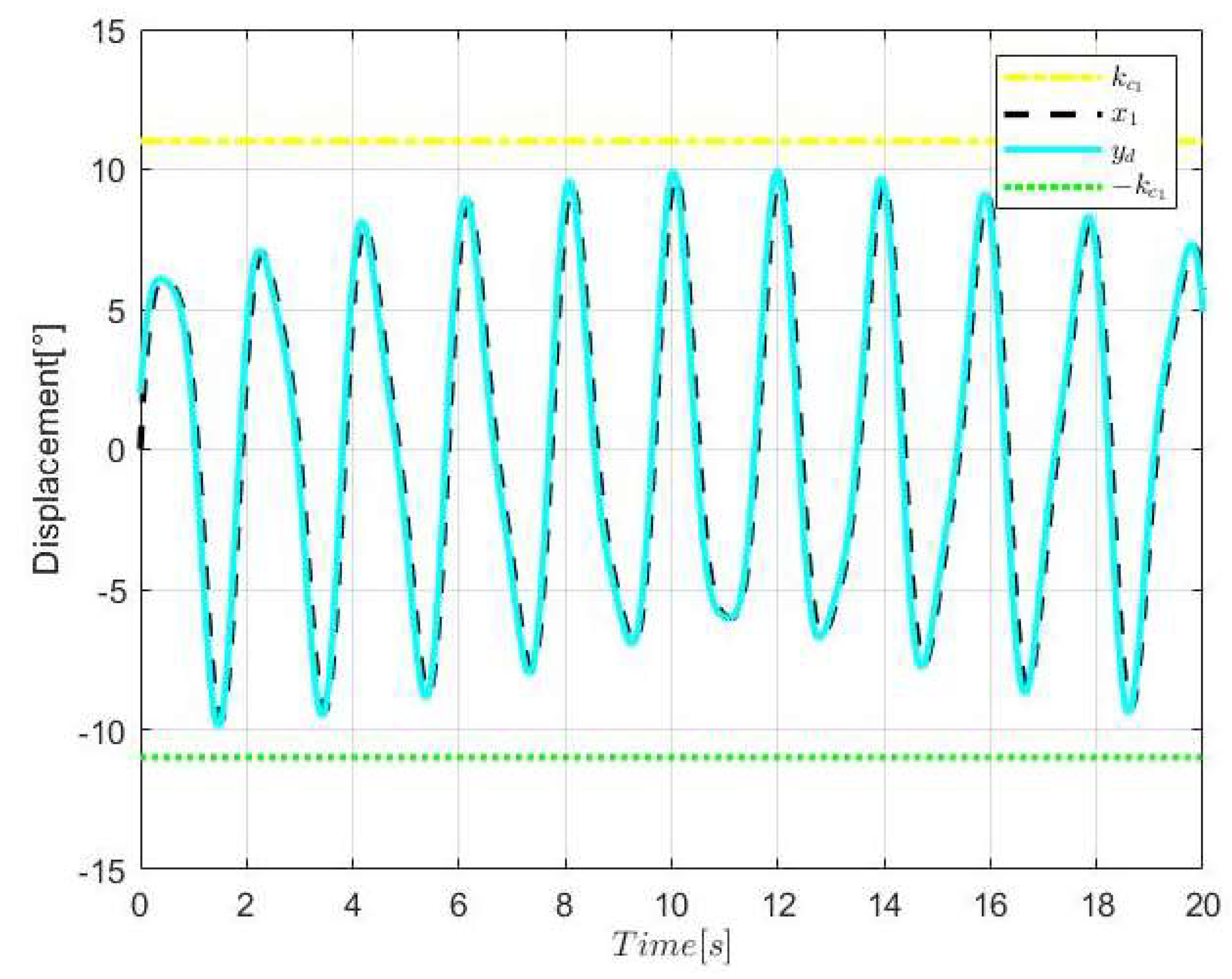
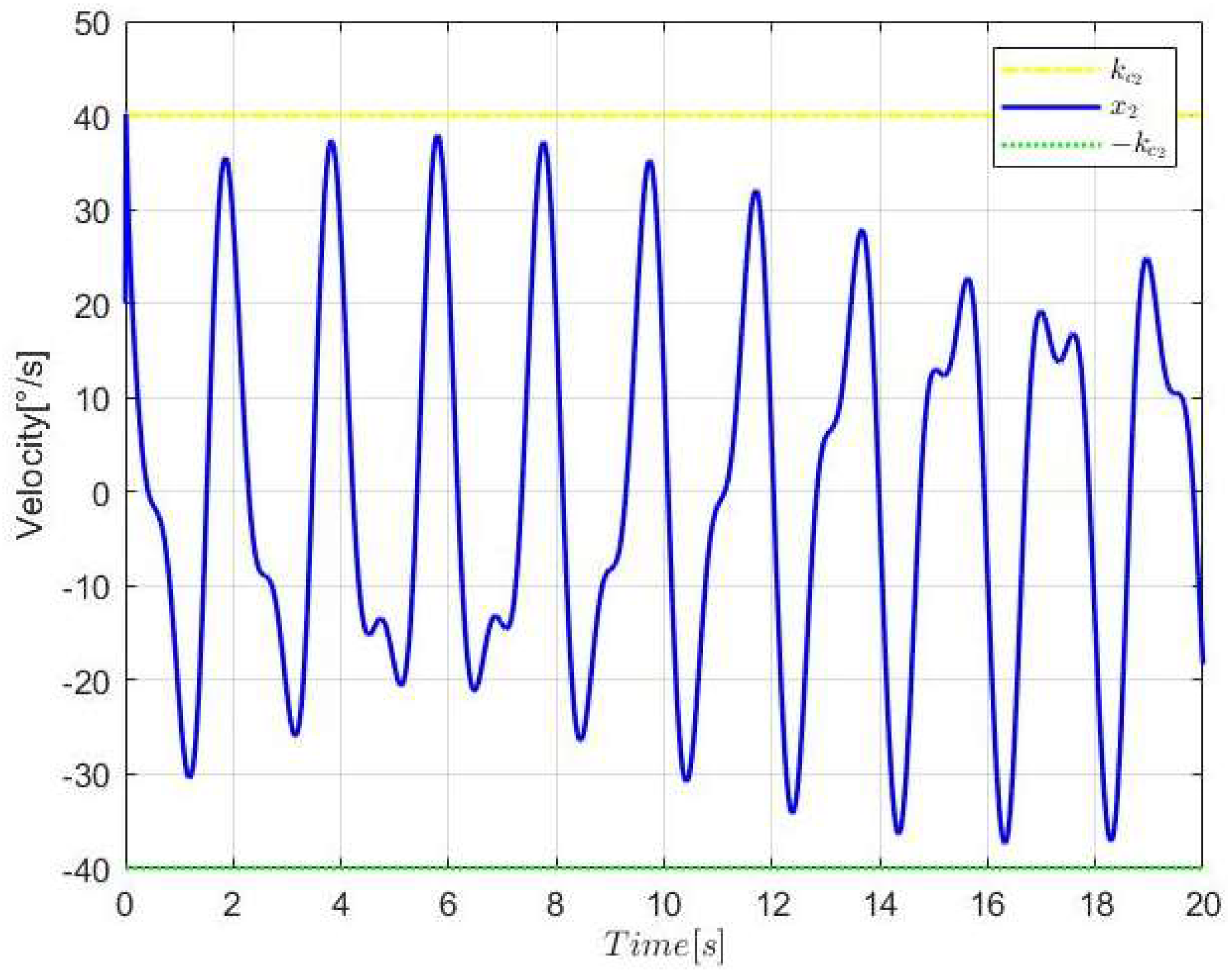
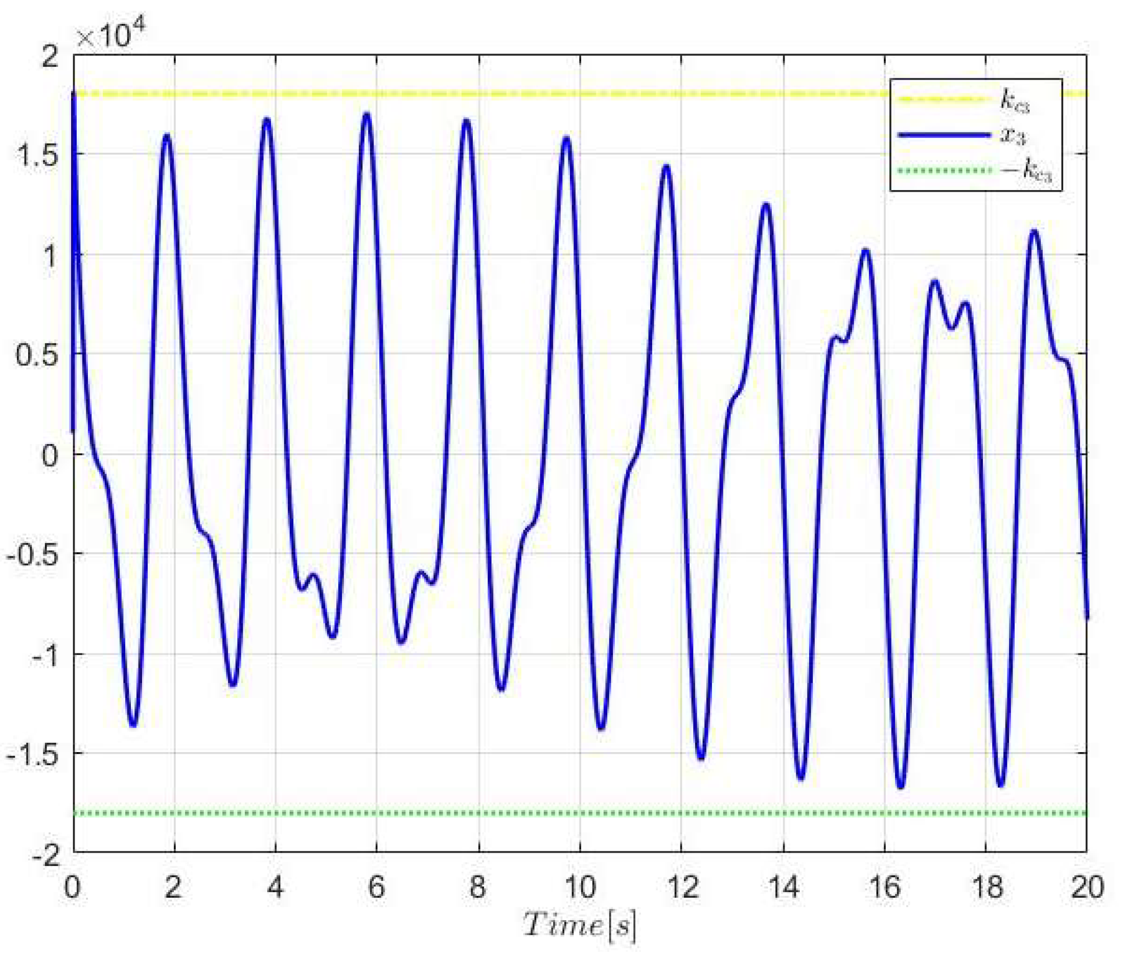
4. Simulation Studies

In order to verify the effectiveness of the proposed neural adaptive controller, computer simulations are carried out. In the simulations, parameters of the electro-hydraulic system to be controlled are chosen with reference to a previous study [5], which are listed in

Table 1. Parameters of the Simulation System.

Physical Parameter	Value
$J(\mathrm{k}\mathrm{g}\cdot {\mathrm{m}}^2)$	$0.2$
$D_m({\mathrm{m}}^3/\mathrm{r}\mathrm{a}\mathrm{d})$	$5.8\times {10}^{-5}$
$C_t({\mathrm{m}}^3/\mathrm{s}/\mathrm{P}\mathrm{a})$	$1.0\times {10}^{-12}$
$k_t({\mathrm{m}}^3/\mathrm{s}/\mathrm{V}/\mathrm{P}{\mathrm{a}}^{-1/2})$	$1.1969\times {10}^{-8}$
$B(\mathrm{N}\cdot \mathrm{m}\cdot \mathrm{s}/\mathrm{r}\mathrm{a}\mathrm{d})$	$90$
${\beta }_e(\mathrm{P}\mathrm{a})$	$7.0\times {10}^8$
$V_t({\mathrm{m}}^3)$	$1.16\times {10}^{-4}$
$P_s(\mathrm{P}\mathrm{a})$	$1.0\times {10}^7$

.

The two layers’ RBFNNs ${\widehat{f}}_1(x_2|{\widehat{W}}_1)={\widehat{W}}_1^T{S}_1(x_2)$ and ${\widehat{f}}_2(Z_2|{\widehat{W}}_1)={\widehat{W}}_2^T{S}_2(Z_2)$ contain five nodes with the centers spaced in the interval [−2, 2] and the widths of the Gaussian function are selected as 5. The radial basis functions are chosen as follows.

$$s_{1,j}(x_2)=\exp \left[-\frac{{(x_2-o_{1,j})}^2}{5}\right]$$

(46)

$$s_{2,j}(x_2,x_3)=\exp \left[-\frac{{(x_2-o_{2,j})}^2}{5}\right]\times \exp \left[-\frac{{(x_3-o_{2,j})}^2}{5}\right]$$

(47)

where $o_{1,j}=-3+j,j=1,\dots ,5$ are centers of the nodes in RBFNN ${\widehat{f}}_1(x_2|{\widehat{W}}_1)={\widehat{W}}_1^T{S}_1(x_2)$, $o_{2,j}=-3+j,j=1,\dots ,5$ are centers of the nodes in RBFNN ${\widehat{f}}_2(Z_2|{\widehat{W}}_1)={\widehat{W}}_2^T{S}_2(Z_2)$.

The virtual control laws and the actual controller are designed as follows

$${\alpha }_1={\dot{y}}_d-c_1{z}_1$$

(48)

$${\alpha }_2=-c_2{z}_2-{\widehat{W}}_1{}^T{S}_1(Z_1)-\frac{z_2}{k_{b2}^2-z_2^2}-\frac{k_{b2}^2-z_2^2}{k_{b1}^2-z_1^2}{z}_1+{\dot{\alpha }}_1$$

(49)

$$u=-\frac{1}{g(x_3,u)}\left[k_3{z}_3+{\widehat{W}}_2{}^T{S}_2(Z_2)+\frac{z_3}{k_{b3}^2-z_3^2}+\frac{\left(k_{b3}^2-z_3^2\right)}{\left(k_{b2}^2-z_2^2\right)}{z}_2+\Xi \right]$$

(50)

where

$$\begin{array}{l}\Xi =\frac{\partial {\alpha }_2}{\partial x_1}{x}_2+\frac{\partial {\alpha }_2}{\partial x_2}{x}_3+\frac{\partial {\alpha }_2}{\partial {\widehat{W}}_1}{\dot{\widehat{W}}}_1+\frac{\partial {\alpha }_2}{\partial y_d}{\dot{y}}_d+\frac{\partial {\alpha }_2}{\partial {\dot{y}}_d}{\ddot{y}}_d\\ -\frac{z_3}{k_{b3}^2-z_3^2}{\left(\frac{\partial {\alpha }_2}{\partial x_2}\right)}^2-\frac{z_3}{2\left(k_{b3}^2-z_3^2\right)}{\left(\frac{\partial {\alpha }_2}{\partial x_2}\right)}^2{‖S_1(x_2)‖}^2\end{array}$$

The parameter adaptive laws are given as

$${\dot{\widehat{W}}}_1=\frac{1}{{\sigma }_1}\left(\frac{z_2}{k_{b2}^2-z_2^2}{S}_1(x_2)-{\tau }_1{\widehat{W}}_1\right)$$

(51)

$${\dot{\widehat{W}}}_2=\frac{1}{{\sigma }_2}\left(\frac{z_3}{k_{b3}^2-z_3^2}{S}_2(Z_2)-{\tau }_2{\widehat{W}}_2\right)$$

(52)

The design parameters in (48)–(52) are listed in

Table 2. Design Parameters.

	Parameters	Values
Parameters of the virtual and actual controllers	$c_1$	$226$
	$c_2$	$215$
	$c_3$	$256$
Parameters of parameter adaptive laws	${\sigma }_1^{-1}$	$1.7$
	${\sigma }_2^{-1}$	$1.5$
	${\tau }_1$	$2.6$
	${\tau }_2$	$2.3$

.

The desired trajectory is selected as $y_d(t)=\left(8\sin (3.28t)+2\cos (6.28t)\right)°$, and the state constraints are given as $\left|x_1\right|\le k_{c1}=11°$, $\left|x_2\right|\le k_{c2}=40°/\mathrm{s}$ and $\left|x_3\right|\le k_{c3}=18000\mathrm{N}/(\mathrm{r}\mathrm{a}\mathrm{d}\cdot \mathrm{k}\mathrm{g}\cdot \mathrm{m})$.

In the simulation, the initial values of the state variables are given as $x_1(0)=2°, x_2(0)=10°/\mathrm{s}, x_3(0)=10000\mathrm{N}/(\mathrm{r}\mathrm{a}\mathrm{d}\cdot \mathrm{k}\mathrm{g}\cdot \mathrm{m})$, while the initial values of the adaptive parameters $W_1$ and $W_2$ are selected as $W_1(0)={[1,2,3,8,2]}^T$, $W_2(0)={[10,8,1,7,15]}^T$.

The simulation results are shown in Figure 3, Figure 4, Figure 5, Figure 6 and Figure 7. Figure 3 shows the trajectories of the output and tracking signals. It can be seen from Figure 3 that the proposed scheme has a good tracking performance. Figure 4 and Figure 5 draw the trajectories of $x_2$ and $x_3$. Figure 3, Figure 4 and Figure 5 illustrate that the given constraint bounds of the state variables are not violated. Figure 6 and Figure 7 depict the trajectories of the actual controller $u(t)$, parameters ${\widehat{W}}_1$ and ${\widehat{W}}_2$, respectively.

Furthermore, to illustrate the effectiveness of the proposed adaptive NN control scheme, we made a simulation comparison with an adaptive control scheme without the state constraints. In the simulation, all the design parameters and initial conditions of the states and parameters are chosen the same as in the above simulation. The simulation results are shown in Figure 8, Figure 9, Figure 10 and Figure 11.

Comparing Figure 3 and Figure 8, it is easy to find that the two control schemes can both guarantee good tracking performance, but the proposed scheme has a more satisfactory performance. By analyzing Figure 3, Figure 4, Figure 5, Figure 8, Figure 9 and Figure 10 we can find that the proposed control scheme can sustain the states $x_i, i=1,2,3$ not to surpass their bounds $k_{ci}$. While the states of the adaptive NN scheme without state constraint violate their bounds in transient conditions. In fact, the state variables surge in the beginning and slightly surpass the constraints, which means that the angular velocity and the load pressure surge too high in the transient conditions, which will do harm to the normal operation of EHS. In addition, from Figure 6 and Figure 11, we can see that the control signal of the proposed adaptive NN control scheme is kept in a reasonable scope of [−3, 3]. However, the input voltage in the adaptive NN control scheme without state constraints spreads in the interval of [14,21], which indicates that the adaptive NN control scheme with state constraints requires less control energy to stabilize the electro-hydraulic system than the one without state constraints.

5. Conclusions

This paper investigated an adaptive NN backstepping control problem for an electro-hydraulic system driven by a dual-vane hydraulic rotary actuator, in which the states are fully constrained, and the friction and internal leakage are nonlinear uncertainties. The neural networks are exploited to approximate the unknown nonlinear uncertainties, and by constructing suitable barrier Lyapunov functions, a novel adaptive NN backstepping control scheme has been developed, which can guarantee the controlled electro-hydraulic system to be stable and the tracking error to converge to a smaller neighborhood of zero. Meanwhile, the state variables are constrained in bounded compact sets. Comparative simulation results have checked the effectiveness of the proposed control method. Our further research work will focus on the finite-time intelligent output control design for electro-hydraulic systems with unmeasurable states.

References

1. Guan, C.; Pan, S. Nonlinear adaptive robust control of single-rod electro-hydraulic actuator with unknown nonlinear parameters. IEEE Trans. Control Syst. Technol. 2008, 16, 434–445. [Google Scholar] [CrossRef]
2. Guan, C.; Pan, S. Adaptive sliding mode control of electro-hydraulic system with nonlinear unknown parameters. Control Eng. Pract. 2008, 16, 1275–1284. [Google Scholar] [CrossRef]
3. Ding, R.; Cheng, M.; Jiang, L.; Hu, G. Active fault-tolerant control for electro-hydraulic systems with an independent metering valve against valve faults. IEEE Trans. Ind. Electron. 2021, 68, 7221–7232. [Google Scholar] [CrossRef]
4. Guo, Q.; Zhang, Y.; Celler, B.G.; Su, S.W. Backstepping control of electro-hydraulic system based on extended-state-observer with plant dynamics largely unknown. IEEE Trans. Ind. Electron. 2016, 63, 6909–6920. [Google Scholar] [CrossRef]
5. Yao, J.; Jiao, Z.; Ma, D. Extended-state-observer-based output feedback nonlinear robust control of hydraulic systems with backstepping. IEEE Trans. Ind. Electron. 2014, 61, 6285–6293. [Google Scholar] [CrossRef]
6. Yao, B.; Bu, F.; Reedy, J.; Chiu, G.T.C. Adaptive robust motion control of single-rod hydraulic actuators: Theory and experiments. IEEE/ASME Trans. Mechatron. 2000, 5, 79–91. [Google Scholar]
7. Yao, J.; Jiao, Z.; Ma, D.; Yan, L. High-accuracy tracking control of hydraulic rotary actuators with modelling uncertainties. IEEE/ASME Trans. Mechatron. 2014, 19, 633–641. [Google Scholar] [CrossRef]
8. Yao, J.; Jiao, Z.; Ma, D. A practical nonlinear adaptive control of hydraulic servomechanisms with periodic-like disturbances. IEEE/ASME Trans. Mechatron. 2015, 20, 2752–2760. [Google Scholar] [CrossRef]
9. Won, D.; Kim, W.; Shin, D.; Chung, C.C. High-gain disturbance observer-based backstepping control with output tracking error constraint for electro-hydraulic systems. IEEE Trans. Control Syst. Technol. 2015, 23, 787–795. [Google Scholar] [CrossRef]
10. Nie, S.; Qian, L.; Chen, L.; Tian, L.; Zou, Q. Barrier Lyapunov functions-based dynamic surface control with tracking error constraints for ammunition manipulator electro-hydraulic system. Def. Technol. 2021, 17, 836–845. [Google Scholar] [CrossRef]
11. Song, Y.; Hu, Z.; Ai, C. Fuzzy Compensation and Load Disturbance Adaptive Control Strategy for Electro-Hydraulic Servo Pump Control System. Electronics 2022, 11, 1159. [Google Scholar] [CrossRef]
12. Botmart, T.; Sabir, Z.; Raja, M.A.Z.; Weera, W.; Sadat, R.; Ali, M.R. A Numerical Study of the Fractional Order Dynamical Nonlinear Susceptible Infected and Quarantine Differential Model Using the Stochastic Numerical Approach. Fractal Fract. 2022, 6, 139. [Google Scholar] [CrossRef]
13. Sabir, Z.; Botmart, T.; Raja, M.A.Z.; Weera, W.; Sadat, R.; Ali, M.R.; Alsulami, A.A.; Alghamdi, A. Artificial neural network scheme to solve the nonlinear influenza disease model. Biomed. Signal Processing Control 2022, 75, 103594. [Google Scholar] [CrossRef]
14. Sabir, Z.; Baleanu, D.; Ali, M.R.; Sadat, R. A novel computing stochastic algorithm to solve the nonlinear singular periodic boundary value problems. Int. J. Comput. Math. 2022. [CrossRef]
15. Zhang, Z.; Peng, L.; Zhang, J.; Wang, X. Finite-Time Neural Network Fault-Tolerant Control for Robotic Manipulators under Multiple Constraints. Electronics 2022, 11, 1343. [Google Scholar] [CrossRef]
16. Costa Branco, P.J.; Dente, J.A. On using fuzzy logic to integrate learning mechanisms in an electro-hydraulic system. I. actuator’s fuzzy modeling. IEEE Trans. Syst. Man Cybern. Part C (Appl. Rev.) 2000, 30, 305–316. [Google Scholar]
17. Guo, Q.; Chen, Z. Neural adaptive control of single-rod electrohydraulic system with lumped uncertainty. Mech. Syst. Signal Processing 2021, 146, 106869. [Google Scholar] [CrossRef]
18. Min, H.; Xu, S.; Zhang, Z. Adaptive finite-time stabilization of stochastic nonlinear systems subject to full-state constraints and input saturation. IEEE Trans. Autom. Control 2021, 66, 1306–1313. [Google Scholar] [CrossRef]
19. Chen, S.; Wu, Y.; Luk, B.L. Combined genetic algorithm optimization and regularized orthogonal least squares learning for radial basis function networks. IEEE Trans. Neural Netw. 1999, 10, 1239–1243. [Google Scholar] [CrossRef] [Green Version]
20. Li, Y.; Wang, T.; Liu, W.; Tong, S. Neural network adaptive output-feedback optimal control for active suspension systems. IEEE Trans. Syst. Man Cybern. Syst. 2021, 1–12. [Google Scholar] [CrossRef]
21. Li, Y.; Liu, Y.; Tong, S. Observer-based neuro-adaptive optimized control of strict-feedback nonlinear systems with state constraints. IEEE Transactions on Neural Networks and Learning Systems 2021, 1–15. [Google Scholar] [CrossRef] [PubMed]
22. Ren, B.; Ge, S.S.; Tee, K.P.; Lee, T.H. Adaptive neural control for output feedback nonlinear systems using a barrier Lyapunov function. IEEE Trans. Neural Netw. 2010, 21, 1339–1345. [Google Scholar] [PubMed]
23. Liu, Y.-J.; Li, J.; Tong, S.; Chen, C.L.P. Neural network control-based adaptive learning design for nonlinear systems with full-state constraints. IEEE Trans. Neural Netw. Learn. Syst. 2016, 27, 1562–1571. [Google Scholar] [CrossRef] [PubMed]
24. Liu, Y.-J.; Zhao, W.; Liu, L.; Li, D.; Tong, S.; Chen, C.L.P. Adaptive Neural Network Control for a Class of Nonlinear Systems with Function Constraints on States. IEEE Trans. Neural Netw. Learn. Syst. 2021, 1–10. [Google Scholar] [CrossRef] [PubMed]
Figure 1. Architecture of the considered hydraulic system.
Electronics 11 01483 g001
Figure 2. The block diagram of the neural adaptive network control scheme.
Electronics 11 01483 g002
Figure 3. The trajectories of x 1 and y d .
Electronics 11 01483 g003
Figure 4. The trajectory of x 2 .
Electronics 11 01483 g004
Figure 5. The trajectory of x 3 .
Electronics 11 01483 g005
Figure 6. The trajectory of u .
Electronics 11 01483 g006
Figure 7. The trajectories of W ^ 1 and W ^ 2 .
Electronics 11 01483 g007
Figure 8. The trajectory of x 1 in control scheme without state constraints.
Electronics 11 01483 g008
Figure 9. The trajectory of x 2 in control scheme without state constraints.
Electronics 11 01483 g009
Figure 10. The trajectory of x 3 in control scheme without state constraints.
Electronics 11 01483 g010
Figure 11. The trajectory of u in control scheme without state constraints.
Electronics 11 01483 g011