The Application of Improved Harmony Search Algorithm to Multi-UAV Task Assignment

Abstract

In this work, aiming at the problem of cooperative task assignment for multiple unmanned aerial vehicles (UAVs) in actual combat, battlefield tasks are divided into reconnaissance tasks, strike tasks and evaluation tasks, and a cooperative task-assignment model for multiple UAVs is built. Meanwhile, heterogeneous UAV-load constraints and mission-cost constraints are introduced, the UAVs and their constraints are analyzed and the mathematical model is established. The exploration performance and convergence performance of the harmony search algorithm are analyzed theoretically, and the more general formulas of exploration performance and convergence performance are proved. Based on theoretical analysis, an algorithm called opposition-based learning parameter-adjusting harmony search is proposed. Using the algorithm to test the functions of different properties, the value range of key control parameters of the algorithm is given. Finally, four algorithms are used to simulate and solve the assignment problem, which verifies the effectiveness of the task-assignment model and the excellence of the designed algorithm. Simulation results show that while ensuring proper assignment, the proposed algorithm is very effective for the multi-objective optimization of heterogeneous UAV-cooperation mission planning with multiple constraints.

1. Introduction

It is very common to use multiple unmanned aerial vehicles to perform various tasks [1,2], especially military tasks [3]. UAVs cooperatively patrolling perimeters, monitoring areas of interest or escorting convoys have been key research topics [4,5,6]. Power inspection, air rescue, large parties and so on are the most common application examples of Multi-UAV cooperation [7,8,9]. Therefore, it is an important research aspect to seek an efficient task-assignment mechanism to solve the task assignment problem of multiple UAVs [10]. In this context, the problem of multi-UAV cooperative task allocation arises at the historic moment.

Collaborative task assignment of multiple UAVs is to assign one or more tasks to UAVs under various constraints in the battlefield environment and determine the sequence of tasks to be executed by UAVs. Task assignment is an important part of collaborative task planning of multiple UAVs, and is also the prerequisite for realizing collaborative operation of UAV groups [11]. In the allocation process, factors such as the type of tasks, timing constraints among tasks, types of tasks that can be performed by UAVs, combat capabilities and payloads should be fully considered, and combat tasks should be reasonably assigned to the UAV fleet with the goal of achieving optimal efficiency of all tasks [12,13]. Therefore, the collaborative task-assignment problem of multiple UAVs is a non-deterministic polynomial (NP) problem of combinatorial optimization under multiple constraints [14,15]. The key to solving this problem is to establish the task assignment model and use the assignment algorithm.

At present, many general mathematical models have been proposed for multi-UAV task allocation at home and abroad. The commonly used task-allocation models include the multiple traveling salesman problem (MTSP) [16] model, mixed-integer linear programming (MILP) model [17], the vehicle routing problem (VRP) [18] model, the network flow optimization (DNFO) [19] model, the cooperative multiple task assignment problem (CMTAP) [20] model, and the capacitated vehicle routing problem (CVRP) [21] model. Based on these general multi-UAV task-allocation models, many scholars have established targeted task-planning models.

However, the current research still has the following problems: (a) In the establishment of qualified task-allocation models, such as the MTSP model and the CVRP model, the requirements of the actual battlefield are ignored in order to meet the model standards. The established model simplifies the objectives of task allocation and battlefield constraints, which reduces the application effect of research results in actual combat. (b) UAV and task types in existing task-allocation models are mostly single, lacking consideration of heterogeneous UAV attributes and multi-task types. Existing UAVs in the formation are different from each other in terms of purpose, load, combat capability, etc. In actual combat, multiple types of UAVs are often needed to cooperate to complete a certain task. Therefore, the task-allocation model based on a single UAV does not support complex tasks.

In solving problem models, there are two main research results: optimization method and heuristic method. The optimization methods include linear programming, width/depth preference search, branch and bound, and so on. The optimization method has a high time and space complexity in solving problems. As the scale of a task-assignment problem increases, computing power is required and the time consumed is also increased. It is thus necessary to simplify the model to a large extent, which makes it difficult to apply to complex problems. The heuristic method of solving a model mainly focuses on the model’s objective function, which requires less complexity. This can result in a better feasible solution in a short time, and has practical feasibility for large-scale complex problems.

The harmony search (HS) algorithm not only has the advantages of a meta-heuristic algorithm, but also own its characteristics [22,23]: (a) HS integrates all the existing harmony vectors to create a new harmony vector, in contrast to GA, which uses two elderly vectors, while particle swarm optimization (PSO) only considers the individual optimal position and the global optimal position of the whole population; (b) HS independently adjusts each variable via improvisation, unlike PSO, which deals with a solution vector by single rule. Due to these characteristics, HS has been successfully applied to a wide variety of optimization problems, such as river ecosystems [24], selective assembly problems [25], mental health analysis [26], reservoir engineering [27], speech emotion [28] and wireless network positioning [29].

However, HS suffers from trapping in performing local searches, and a crucial factor of its performance is the key control parameters, such as harmony memory (HM), harmony memory size (HMS), harmony memory considering rate (HMCR), pitch adjusting rate (PAR), bandwidth (bw) and the number of improvisations (G). It is unfortunate that there are few studies on the mathematical theory of the underlying search mechanisms of HS in the open literature. S. Das et al. proposed a new algorithm called EHS, after discussing the relationship between the explorative power of HS and the control parameters through analyzing the evolution of the population variance of HS [30]. This algorithm has good exploration, but poor exploitation. Thus, this paper devotes significantly more attention to the search mechanism of HS and its parameters.

Therefore, the contribution of this paper is the proposal of a new model and a new method, which aim to: (a) considering the complexity of the actual missions, divide the missions into reconnaissance, strike and evaluation tasks, and considering the benefits, costs and constraints of the missions, establish the target allocation model of heterogeneous multi-UAV missions with different loads; (b) analyze the mathematical theory of the underlying search mechanisms of HS to balance exploration and exploitation, establish the iteration equation of HS and propose an improved HS; (c) use the improved HS algorithm to simulate and verify a multi-UAV task-allocation combat example.

The remainder of this paper is organized as follows. In Section 2, the modeling of heterogeneous UAV task-assignment planning is presented in detail. Section 3 is the theoretical analysis of harmony search. The proposed algorithm is described in Section 4. The experiments and their results of the proposed algorithm are presented in Section 5. The task-allocation simulation experiment is designed and discussed in Section 6. Section 7 discusses related work. Section 8 then makes concluding remarks and indicates future works.

2. Modeling Heterogeneous UAV Task Assignment Planning

Multi-UAV cooperative task assignment is a complex multi-objective optimization and decision problem. Most current research models assume that the mission attributes of UAVs are consistent. However, multi-UAV formation is not a linear addition of a certain number of individual UAVs. Heterogeneous formation disperses the functions of reconnaissance and surveillance, electronic interference, strike and evaluation into a large number of single UAVs with low cost and single function. Through the high level of cooperation and self-organization among a large number of heterogeneous individuals, the cluster function far exceeds the individual function that can be realized. In addition, as the multi-UAV formation combat involves various aspects of the combat target and the task complexity is different, some large tasks need a certain combat sequence, and it is necessary to deploy and combine UAVs with different functions and characteristics to complete the corresponding combat task. For the above reasons, this section proposes a heterogeneous multi-UAV task-allocation model to enhance the antagonism of combat subjects and achieve higher-formation combat effectiveness in view of future diversified combat requirements.

2.1. Objective Function of Multi-UAV Cooperative Target Assignment Model

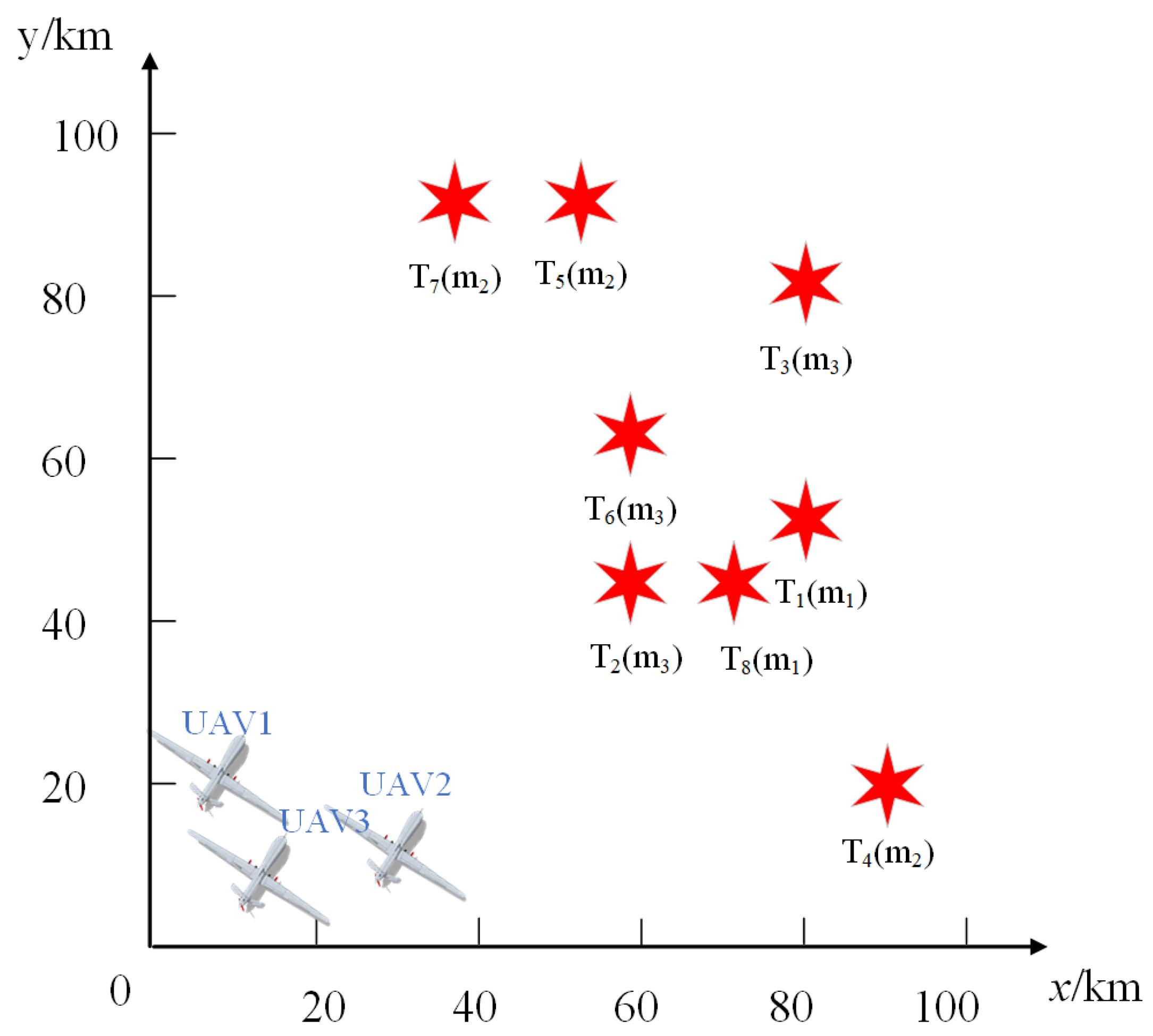
If the UAV formation of our side performs the task $\mathbf{U}=({\mathbf{U}}_1,{\mathbf{U}}_2,{\mathbf{U}}_3,\dots ,{\mathbf{U}}_{{\mathbf{N}}_{\mathbf{UVA}}})$, the target list of the task is $\mathbf{T}=({\mathbf{T}}_1,{\mathbf{T}}_2,{\mathbf{T}}_3,\dots ,{\mathbf{T}}_{{\mathbf{N}}_{\mathbf{TARGET}}})$, $\mathbf{M}=\{{\mathbf{M}}_1,{\mathbf{M}}_2,{\mathbf{M}}_3\}$ represents the task type, ${\mathbf{N}}_{\mathbf{UVA}}$ and ${\mathbf{N}}_{\mathbf{TARGET}}$ are the number of UAVs in the formation and the number of targets in the task list respectively, ${\mathbf{M}}_1$ represents reconnaissance, ${\mathbf{M}}_2$ represents attack and ${\mathbf{M}}_3$ represents evaluation. The essence of multi-UAV formation task assignment is to solve a target-assignment scheme to maximize target fitness ($\mathbf{Tar}\_\mathbf{fitness}$). Based on this, the objective function of a multi-UAV cooperative target-allocation model is given as follows

Definition 1.

$$\mathbf{Tar}\_{\mathbf{fitness}}_{\mathbf{i}}({\mathbf{T}}_{\mathbf{j}})={\mathbf{Reward}}_{\mathbf{i}}({\mathbf{T}}_{\mathbf{j}})/{\mathbf{Cost}}_{\mathbf{i}}({\mathbf{T}}_{\mathbf{j}}).$$

(1)

where$\mathbf{Tar}\_{\mathbf{fitness}}_{\mathbf{i}}({\mathbf{T}}_{\mathbf{j}})$isthe fitnessof the UAV numbered$\mathbf{i}$performing the task numbered$\mathbf{j}$,${\mathbf{Reward}}_{\mathbf{i}}({\mathbf{T}}_{\mathbf{j}})$isthe rewardof the UAV numbered$\mathbf{i}$performing the task numbered$\mathbf{j}$and${\mathbf{Cost}}_{\mathbf{i}}({\mathbf{T}}_{\mathbf{j}})$isthe costof the UAV numbered$\mathbf{i}$performing the task numbered$\mathbf{j}$. It can be seen that task fitnessis directly proportional to the reward of performing tasks and inversely proportional to the cost of performing tasks.

2.2. Task Rewards Modeling

In this paper, the rewards of UAV numbered $\mathbf{i}$ performing a certain task numbered $\mathbf{j}$ are mainly determined by three factors:

(1) UAV’s capability to perform specific tasks. The capability of UAV to perform tasks is quantified by its payload, such as detection device and weapon system, combined with its own performance, and described in probability based on historical experience (whether it has performed relevant target tasks in the past).

(2) the worth of enemy targets. The worth of enemy targets is determined in advance based on the information obtained beforehand, combined with the tactical plan available for reference. For example, destroying the enemy’s command center can paralyze the enemy’s operation, so the worth of the command center is relatively high, while striking the enemy’s small warehouse has relatively low worth compared to the whole operation.

(3) the defense capability of enemy targets. Combined with the detected battlefield environment information and advance intelligence information, the enemy targets, such as surface-to-air missile positions, anti-aircraft gun positions, flight bases and ground radar are analyzed and quantified.

From the above analysis, the mission rewards of UAV can be defined as follows:

Definition 2.

$${\mathbf{Reward}}_{\mathbf{i}}({\mathbf{T}}_{\mathbf{j}})=\frac{\mathbf{Worth}({\mathbf{T}}_{\mathbf{j}})·{\mathbf{P}}_{\mathbf{i}}({\mathbf{T}}_{\mathbf{j}})}{\mathbf{Defence}({\mathbf{T}}_{\mathbf{j}})}.$$

(2)

where${\mathbf{Reward}}_{\mathbf{i}}({\mathbf{T}}_{\mathbf{j}})$is the rewards of a certain task numbered$\mathbf{j}$performed by a UAV numbered$\mathbf{i}$with a specific load,${\mathbf{P}}_{\mathbf{i}}({\mathbf{T}}_{\mathbf{j}})$is the completion capability of the UAV numbered$\mathbf{i}$to perform tasks the task numbered$\mathbf{j}$and$\mathbf{Defence}({\mathbf{T}}_{\mathbf{j}})$is the defense capability of the target.

The reward of each UAV mission meets the additivity, and the decision variable of the mission is introduced as follows:

$${\mathbf{x}}_{\mathbf{i}\mathbf{j}}=\left\{\begin{array}{l}1, \mathbf{UAV}\mathbf{i} \mathbf{performs} \mathbf{the} \mathbf{task} \mathbf{j}\\ 0, \mathbf{UAV}\mathbf{i} \mathbf{does} \mathbf{not} \mathbf{perform} \mathbf{the} \mathbf{task} \mathbf{j}\end{array}\right.,$$

(3)

Then, the total rewards of multiple UAV formation’s task execution on the target list are:

$$\mathbf{Reward}={\displaystyle \sum _{\mathbf{j}=1}^{{\mathbf{N}}_{\mathbf{TARGET}}}{\displaystyle \sum _{\mathbf{i}=1}^{{\mathbf{N}}_{\mathbf{UVA}}}{\mathbf{x}}_{\mathbf{i}\mathbf{j}}}}{\mathbf{Reward}}_{\mathbf{i}}({\mathbf{T}}_{\mathbf{j}}),$$

(4)

2.3. Task Cost Modeling

In the course of reconnaissance, attack or evaluation, UAV formation will encounter confrontational threats and terrain threats. Confrontational threats are mainly radar detection and fire attack by enemy targets during the execution of missions, so the defense capability of our UAV and the attack capability of enemy targets should be considered in task allocation. Terrain threats mainly involve the air-range cost of a UAV during its mission, terrain height and altitude change rate. On some terrain that is difficult to leap over, the UAV flying too high will consume too much energy, and the UAV climbing too-steep terrain is likely to impact the terrain and encounter other threats, so it should try to avoid the distribution results of too-long air-range or steep terrain. Based on the above analysis, the task-cost modeling in this section includes terrain-cost modeling and loss-cost modeling. At the same time, terrain cost and loss cost of different dimensions are normalized.

(1) Terrain Cost

The air-range cost of a UAV reflects the duration of the mission, the length of the UAV and the energy consumption. The Euclidean distance between the UAV and the enemy target is used in this paper to estimate the air-range cost. This is because the formation cannot accurately obtain the relevant data before the actual execution of the mission.

$$\left\{\begin{array}{l}\mathbf{DisU}{\mathbf{T}}_{\mathbf{i}\mathbf{j}}=\sqrt{{\left(\mathbf{Po}{\mathbf{s}}_{\mathbf{x}}\left({\mathbf{U}}_{\mathbf{i}}\right)-\mathbf{Po}{\mathbf{s}}_{\mathbf{x}}\left({\mathbf{T}}_{\mathbf{i}}\right)\right)}^2+{\left(\mathbf{Po}{\mathbf{s}}_{\mathbf{y}}\left({\mathbf{U}}_{\mathbf{i}}\right)-\mathbf{Po}{\mathbf{s}}_{\mathbf{y}}\left({\mathbf{T}}_{\mathbf{i}}\right)\right)}^2}\\ \mathbf{DisT}{\mathbf{T}}_{\mathbf{i}\mathbf{j}}=\sqrt{{\left(\mathbf{Po}{\mathbf{s}}_{\mathbf{x}}\left({\mathbf{T}}_{\mathbf{i}}\right)-\mathbf{Po}{\mathbf{s}}_{\mathbf{x}}\left({\mathbf{T}}_{\mathbf{j}}\right)\right)}^2+{\left(\mathbf{Po}{\mathbf{s}}_{\mathbf{y}}\left({\mathbf{T}}_{\mathbf{i}}\right)-\mathbf{Po}{\mathbf{s}}_{\mathbf{y}}\left({\mathbf{T}}_{\mathbf{j}}\right)\right)}^2}\end{array}\right.,$$

(5)

where $\left(\mathbf{Po}{\mathbf{s}}_{\mathbf{x}}\left({\mathbf{U}}_{\mathbf{i}}\right),\mathbf{Po}{\mathbf{s}}_{\mathbf{y}}\left({\mathbf{U}}_{\mathbf{i}}\right)\right)$ is the initial position coordinate of the UAV numbered $\mathbf{i}$, $\left(\mathbf{Po}{\mathbf{s}}_{\mathbf{x}}\left({\mathbf{T}}_{\mathbf{i}}\right),\mathbf{Po}{\mathbf{s}}_{\mathbf{y}}\left({\mathbf{T}}_{\mathbf{i}}\right)\right)$ is the position coordinate of the enemy target numbered $\mathbf{i}$, $\left(\mathbf{Po}{\mathbf{s}}_{\mathbf{x}}\left({\mathbf{T}}_{\mathbf{j}}\right),\mathbf{Po}{\mathbf{s}}_{\mathbf{y}}\left({\mathbf{T}}_{\mathbf{j}}\right)\right)$ is the position coordinate of the enemy target numbered $\mathbf{j}$. Equation (5) gives the Euclidean distance between the UAV numbered $\mathbf{i}$ and the task target numbered $\mathbf{j}$, as well as the Euclidean distance between the task numbered $\mathbf{i}$ and the task numbered $\mathbf{j}$. To facilitate calculation, the matrix $\mathbf{Range}$ is established as the distance matrix.

$$\mathbf{Range}=\left[\begin{array}{cc}\hfill & \mathbf{DisU}{\mathbf{T}}_{1,1}\hspace{0.33em}\hspace{0.33em}\hspace{0.33em}\hspace{0.33em}\cdots \hspace{0.33em}\hspace{0.33em}\hspace{0.33em}\hspace{0.33em}\mathbf{DisU}{\mathbf{T}}_{1,{\mathbf{N}}_{\mathbf{TARGET}}}\hfill \\ \hfill & \hspace{0.33em}\hspace{0.33em}\hspace{0.33em}⋮\hspace{0.33em}\hspace{0.33em}\hspace{0.33em}\hspace{0.33em}\hspace{0.33em}\hspace{0.33em}\hspace{0.33em}\hspace{0.33em}\hspace{0.33em}\ddots \hspace{0.33em}\hspace{0.33em}\hspace{0.33em}\hspace{0.33em}\hspace{0.33em}\hspace{0.33em}\hspace{0.33em}\hspace{0.33em}\hspace{0.33em}\hspace{0.33em}\hspace{0.33em}⋮\hfill \\ \hfill & \mathbf{DisU}{\mathbf{T}}_{{\mathbf{N}}_{\mathbf{UAV}},1}\hspace{0.33em}\hspace{0.33em}\hspace{0.33em}\cdots \hspace{0.33em}\hspace{0.33em}\hspace{0.33em}\mathbf{DisU}{\mathbf{T}}_{{\mathbf{N}}_{\mathbf{UAV}},{\mathbf{N}}_{\mathbf{TARGET}}}\hfill \\ \hfill & \mathbf{DisT}{\mathbf{T}}_{1,1}\hspace{0.33em}\hspace{0.33em}\hspace{0.33em}\hspace{0.33em}\cdots \hspace{0.33em}\hspace{0.33em}\hspace{0.33em}\hspace{0.33em}\hspace{0.33em}\mathbf{DisT}{\mathbf{T}}_{1,{\mathbf{N}}_{\mathbf{TARGET}}}\hfill \\ \hfill & \hspace{0.33em}\hspace{0.33em}\hspace{0.33em}⋮\hspace{0.33em}\hspace{0.33em}\hspace{0.33em}\hspace{0.33em}\hspace{0.33em}\hspace{0.33em}\hspace{0.33em}\hspace{0.33em}\hspace{0.33em}\ddots \hspace{0.33em}\hspace{0.33em}\hspace{0.33em}\hspace{0.33em}\hspace{0.33em}\hspace{0.33em}\hspace{0.33em}\hspace{0.33em}\hspace{0.33em}\hspace{0.33em}\hspace{0.33em}⋮\hfill \\ \hfill & \mathbf{DisT}{\mathbf{T}}_{{\mathbf{N}}_{\mathbf{UAV}},1}\hspace{0.33em}\hspace{0.33em}\cdots \hspace{0.33em}\hspace{0.33em}\mathbf{DisT}{\mathbf{T}}_{{\mathbf{N}}_{\mathbf{UAV}},{\mathbf{N}}_{\mathbf{TARGET}}}\hfill \end{array}\right]$$

(6)

According to the above equation, $\mathbf{Range}$ is a matrix of $\left({\mathbf{N}}_{\mathbf{UAV}}+{\mathbf{N}}_{\mathbf{TARGET}}\right)\times {\mathbf{N}}_{\mathbf{TARGET}}$, which contains the Euclidean distance between UAV and enemy targets and the Euclidean distance between enemy targets. Thus, the total air-range of the UAV numbered $\mathbf{i}$ returning to its initial position after completing the corresponding task target list can be given as follows:

$${\mathbf{Length}}_{\mathbf{i}}={\displaystyle \sum _{\mathbf{n}=0}^{\mathbf{N}}\mathbf{Length}{\left(\mathbf{i}\right)}_{\mathbf{n},\mathbf{n}+1}},$$

(7)

where $\mathbf{N}$ represents the total number of tasks performed by UAV numbered $\mathbf{i}$. Further analysis of Equation (7): when $\mathbf{n}=0$, $\mathbf{Length}{\left(\mathbf{i}\right)}_{0,1}$ represents the distance between the initial position of the UAV numbered $\mathbf{i}$ and the mission target numbered 1. When $\mathbf{n}=\{1,2,\dots ,\mathbf{N}-1\}$, $\mathbf{Length}{\left(\mathbf{i}\right)}_{\mathbf{n},\mathbf{n}+1}$ represents the Euclidean distance between the No. $\mathbf{n}$ mission target, performed by the UAV numbered $\mathbf{i}$, and the No.$(\mathbf{n}+1)$ mission target. When $\mathbf{n}=\mathbf{N}$,$\mathbf{Length}{\left(\mathbf{i}\right)}_{\mathbf{N}, \mathbf{N}+1}$ represents the distance of UAV numbered $\mathbf{i}$ returning to its starting point after completing the last mission target.

Considering the impact of terrain height and altitude-change rate on the UAV’s loss, terrain-steepness factor λ is introduced to the weighted UAV’s track. Assuming that the battlefield environment can be known in advance before the execution of the mission, the value of the terrain-steepness factor λ is determined by combining the result of task assignment with the terrain information known in advance. In this paper, λ ranges from [1.2, 2.5] according to the complexity of the terrain.

(2) Loss Cost

The loss cost of a UAV is mainly caused by the confrontational threats encountered by UAV in the execution of tasks. Therefore, the loss cost mainly considers the following factors: the worth of UAV with specific load, the defensive capability of UAV itself, and the attack capability of enemy targets. Combined with the significance of loss cost, it can be concluded from the above analysis:

Definition 3.

$$\mathbf{Loss}\mathbf{Cos}{\mathbf{t}}_{\mathbf{i}\mathbf{j}}=\frac{\mathbf{Worth}({\mathbf{U}}_{\mathbf{i}})·\mathbf{Strike}({\mathbf{T}}_{\mathbf{j}})}{\mathbf{Defense}({\mathbf{U}}_{\mathbf{i}})}.$$

(8)

where$\mathbf{Loss}\mathbf{Cos}{\mathbf{t}}_{\mathbf{i}\mathbf{j}}$is the loss cost of the UAV numbered$\mathbf{i}$when executing the mission targetnumbered$\mathbf{j}$,$\mathbf{Strike}({\mathbf{T}}_{\mathbf{j}})$is the attack capability of the mission targetnumbered$\mathbf{j}$,$\mathbf{Worth}({\mathbf{U}}_{\mathbf{i}})$is the worth of UAV numbered$\mathbf{i}$,$\mathbf{Defense}({\mathbf{U}}_{\mathbf{i}})$is the defense capability of UAV numbered$\mathbf{i}$.

Thus, it can be concluded that the task cost of multi-UAV formation in task allocation is as followed:

$$\begin{array}{ll}\mathbf{Cost}& =\mathbf{Terrain}\mathbf{Cost}+ \mathbf{Loss}\mathbf{Cost}\\ & =\hspace{0.33em}{\mathsf{\omega }}_1·{\displaystyle \sum _{\mathbf{i}=1}^{{\mathbf{N}}_{UAV}}{\lambda }_{\mathbf{i}}·\mathbf{Lengt}{\mathbf{h}}_{\mathbf{i}}}+{\mathsf{\omega }}_2·{\displaystyle \sum _{\mathbf{i}=1}^{{\mathbf{N}}_{UAV}}{\displaystyle \sum _{\mathbf{j}=1}^{{\mathbf{N}}_{\mathbf{TARGET}}}{\mathbf{x}}_{\mathbf{i}\mathbf{j}}·}\frac{\mathbf{Loss}\mathbf{Cos}{\mathbf{t}}_{\mathbf{i}\mathbf{j}}}{\mathbf{Loss}\mathbf{Cos}{\mathbf{t}}_{\mathbf{max}}}}\end{array}$$

(9)

where $\mathbf{Loss}\mathbf{Cos}{\mathbf{t}}_{\mathbf{max}}$ is the maximal element with the total loss cost of performing all tasks, ${\lambda }_{\mathbf{i}}$ is the terrain steepness factor reflecting the complexity of different UAV flight paths, ${\mathsf{\omega }}_1$ and ${\mathsf{\omega }}_2$ respectively represent the UAV’s track weight and loss weight and ${\mathbf{x}}_{\mathbf{i}\mathbf{j}}$ is the task decision variables introduced in Section 2.2.

2.4. Modeling Constraints

(1) Constraints on Task Completion

During the execution of the mission, UAVs involved in such tasks as strike and reconnaissance must perform all the missions, and there cannot be a situation where some tasks are not assigned, namely,

$${\displaystyle \sum _{\mathbf{i}=1}^{{\mathbf{N}}_{\mathbf{UAV}}}{\displaystyle \sum _{\mathbf{j}=1}^{{\mathbf{N}}_{\mathbf{TARGET}}}{\mathbf{x}}_{\mathbf{i}\mathbf{j}}={\mathbf{N}}_{\mathbf{TARGET}}}},$$

(10)

where, $\mathbf{i}=\{1,2,\dots ,{\mathbf{N}}_{\mathbf{UAV}}\}$ and $\mathbf{j}=\{1,2,\dots ,{\mathbf{N}}_{\mathbf{TARGET}}\}$ represent the number of UAVs and the number of assigned tasks respectively.

(2) Constraints on Task Non-Redundancy

During task execution, it must be ensured that each task can only be performed by a certain UAV, namely,

$${\displaystyle \sum _{\mathbf{i}=1}^{{\mathbf{N}}_{\mathbf{UAV}}}{\mathbf{x}}_{\mathbf{i}\mathbf{j}}=1},\forall \mathbf{j}=1,2,\dots ,{\mathbf{N}}_{\mathbf{TARGET}}$$

(11)

(3) Constraints on UAV’s Capability

The number of task targets numbered $\mathbf{j}$ performed by the UAV numbered $\mathbf{i}$ should not exceed the maximum of its own task capability:

$${\displaystyle \sum _{\mathbf{j}=1}^{{\mathbf{N}}_{\mathbf{TARGET}}}{\mathbf{x}}_{\mathbf{i}\mathbf{j}}\le }\mathbf{Loa}{\mathbf{d}}_{\mathbf{i}},\forall \mathbf{i}=1,2,\dots ,{\mathbf{N}}_{\mathbf{UAV}},$$

(12)

where $\mathbf{Loa}{\mathbf{d}}_{\mathbf{i}}$ represents the maximum number of tasks that UAV numbered $\mathbf{i}$ can execute.

(4) Constraints on UAV’s Attack Range

When task target assignment is completed, the air-range of the total mission performed by the UAV numbered $\mathbf{i}$ cannot exceed its maximal flight distance, namely:

$${\lambda }_{\mathbf{i}}\cdot \mathbf{Lengt}{\mathbf{h}}_{\mathbf{i}}\le \mathbf{D}{\left(\mathbf{i}\right)}_{\mathbf{max}},\hspace{0.33em}\hspace{0.33em}\forall \mathbf{i}=1,2,\dots ,{\mathbf{N}}_{\mathbf{UAV}},$$

(13)

where ${\lambda }_{\mathbf{i}}$ is the terrain steepness factor, and $\mathbf{D}{\left(\mathbf{i}\right)}_{\mathbf{max}}$ is the maximal air-range of UAV numbered $\mathbf{i}$.

In order to transform constrained optimization problems into unconstrained problems, this section introduces the penalty function and designs an outpoint method to punish the consumption cost of infeasible solutions when infeasible solutions appear in the population. The constrained optimization method improves the efficiency of the task-assignment model. Therefore, Equation (1) is further updated, and the final total task fitness is as follows:

$$\mathbf{Tar}\_\mathbf{fitness}\_\mathbf{final}=\frac{\mathbf{Reward}}{\mathbf{Cost}}-\mathsf{\delta }\cdot \mathbf{Pu},$$

(14)

$$\mathbf{Pu}=\left\{\begin{array}{l}1, \mathbf{when} \mathbf{task} \mathbf{assignment} \mathbf{meets} \mathbf{constraints}\\ 0, \mathbf{when} \mathbf{task} \mathbf{assignment} \mathbf{does} \mathbf{not} \mathbf{meet} \mathbf{constraints}\end{array}\right.,$$

(15)

where $\mathsf{\delta }$ is a positive number known as the penalty factor, and $\mathbf{Pu}$ is the penalty function.

2.5. Task-Assignment Coding

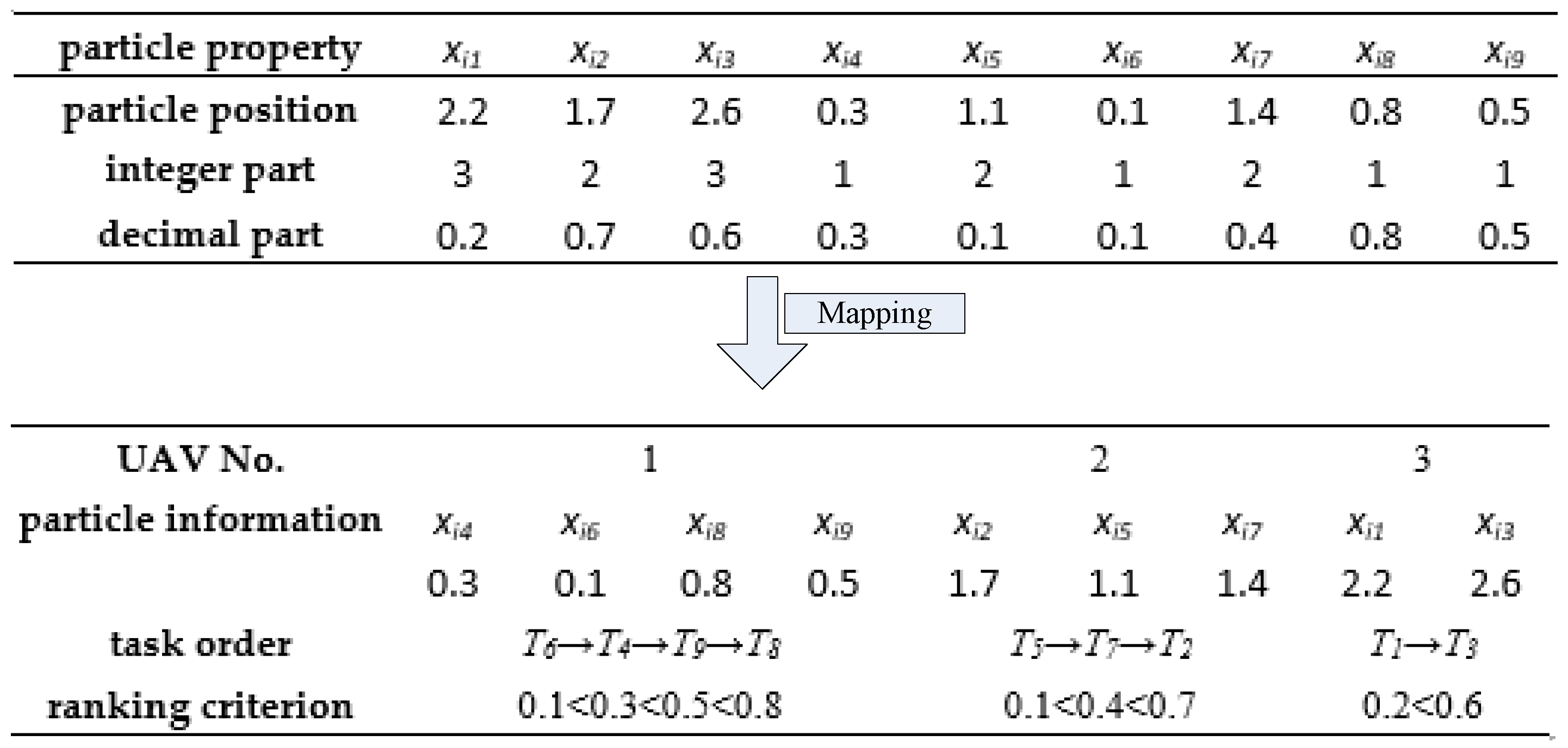
Constructing the mapping relationship between particle and feasible solution of cooperative-task assignment for multiple UAVs is the key step for the swarm intelligence algorithm to solve the optimization problem. In the collaborative-task assignment process for multiple UAVs, the response of the UAVs to enemy target reconnaissance, attack and evaluation tasks should be ensured, and the timing of tasks should also be ensured. That is, an enemy target must be reconnoitered before the attack task, and finally the effect evaluation, which embodies the double-layer coding meaning of particles on the task-assignment problem. Referring to reference [31], this paper adopts real vector coding. Suppose that the dimension of the particle is the number of the task target list, the subscript of the particle corresponds to the number of tasks, the integer part of the particle position is rounded up to indicate the number of UAVs and the fractional part of the particle position corresponds to the task order of UAVs from small to large.

The mapping relationship between particle coding and task target assignment can be expressed by the following example. Suppose that three UAVs must perform nine tasks, and the task-assignment coding is shown in Figure 1.

3. The Theoretical Analysis of Harmony Search

This section analyzes the performance of the HS algorithm from two aspects: exploration performance and iterative convergence performance.

3.1. Exploration Performance

The HS algorithm explores the solution space by improvisation, and its development is accomplished by updating the operation steps. In reference [30], the exploration ability of HS is measured by the evolution of the expected population variance with the number of iterations. However, only symmetric intervals $\left[-\mathbf{a},\mathbf{a}\right]$, $\mathbf{a}\in \mathbf{R}$ are considered for analyzing the evolution of the group variables of HS and its exploration performance. Here, this paper gives results for asymmetric intervals, as shown in Theorem 1.

Theorem 1.

Let$\mathbf{x}=\{{\mathbf{x}}_1,{\mathbf{x}}_2,···,{\mathbf{x}}_{\mathbf{m}}\}$represent the initial population of HS algorithm,$\mathbf{y}=\{{\mathbf{y}}_1,{\mathbf{y}}_2,···,{\mathbf{y}}_{\mathbf{m}}\}$refer to the population obtained after the improvisation session. The range of the decision variable${\mathbf{x}}_{\mathbf{i}}$is$\left[\mathbf{a},\mathbf{b}\right],\mathbf{a},\mathbf{b}\in \mathbf{R}$, then

$$\begin{array}{l}\mathbf{E}(\mathbf{var}(\mathbf{y}))=(1-\frac{1}{\mathbf{HMS}})\cdot [\mathbf{HMCR}\cdot \mathbf{E}(\mathbf{var}(\mathbf{x}))+\mathbf{HMCR}\cdot (1-\mathbf{HMCR})\cdot {(\overline{\mathbf{x}})}^2\\ \hspace{0.33em}\hspace{0.33em}\hspace{0.33em}\hspace{0.33em}\hspace{0.33em}\hspace{0.33em}\hspace{0.33em}\hspace{0.33em}\hspace{0.33em}\hspace{0.33em}\hspace{0.33em}\hspace{0.33em}\hspace{0.33em}\hspace{0.33em}+\frac{\mathbf{b}{\mathbf{w}}^2}{3}\cdot \mathbf{HMCR}\cdot \mathbf{PAR}+\frac{1}{12}(1-\mathbf{HMCR})\cdot {(\mathbf{a}-\mathbf{b})}^2]\end{array}$$

(16)

Proof. 

when $\mathbf{x}\in \left[-\mathbf{a},\mathbf{a}\right],\mathbf{a}\in \mathbf{R}$, the following result as Equation (17) is obtained, which had been done by S. Das et al. in literature [30].

$$\begin{array}{l}\mathbf{E}(\mathbf{var}(\mathbf{y}))=(1-\frac{1}{\mathbf{HMS}})\cdot [\mathbf{HMCR}\cdot \mathbf{E}(\mathbf{var}(\mathbf{x}))+\mathbf{HMCR}\cdot (1-\mathbf{HMCR})\cdot {\left(\overline{\mathbf{x}}\right)}^2\\ \hspace{0.33em}\hspace{0.33em}\hspace{0.33em}\hspace{0.33em}\hspace{0.33em}\hspace{0.33em}\hspace{0.33em}\hspace{0.33em}\hspace{0.33em}\hspace{0.33em}\hspace{0.33em}\hspace{0.33em}+\frac{\mathbf{b}{\mathbf{w}}^2}{3}\cdot \mathbf{HMCR}\cdot \mathbf{PAR}+\frac{{\mathbf{a}}^2}{3}(1-\mathbf{HMCR})]\end{array}$$

(17)

where, Equations (18) and (19) are workable from the proof in literature [30].

$$\begin{array}{l}\mathbf{E}({\mathbf{y}}_{\mathbf{l}})=\mathbf{HMCR}\cdot (1-\mathbf{PAR})\cdot \mathbf{E}({\mathbf{x}}_{\mathbf{r}})+0.5\cdot \mathbf{HMCR}\cdot \mathbf{PAR}\cdot \mathbf{E}({\mathbf{x}}_{\mathbf{r}}+\mathbf{b}\mathbf{w}\cdot \mathbf{rand})\\ \hspace{0.33em}\hspace{0.33em}\hspace{0.33em}\hspace{0.33em}\hspace{0.33em}\hspace{0.33em}\hspace{0.33em}\hspace{0.33em}\hspace{0.33em}+0.5\cdot \mathbf{HMCR}\cdot \mathbf{PAR}\cdot \mathbf{E}({\mathbf{x}}_{\mathbf{r}}-\mathbf{b}\mathbf{w}\cdot \mathbf{rand})+(1-\mathbf{HMCR})\cdot \mathbf{E}({\mathbf{x}}_{\mathbf{new}})\end{array}$$

(18)

$$\begin{array}{l}\mathbf{E}({({\mathbf{y}}_{\mathbf{l}})}^2)=\mathbf{HMCR}\cdot (1-\mathbf{PAR})\cdot \mathbf{E}({({\mathbf{x}}_{\mathbf{r}})}^2)+0.5\cdot \mathbf{HMCR}\cdot \mathbf{PAR}\cdot \mathbf{E}({({\mathbf{x}}_{\mathbf{r}}+\mathbf{b}\mathbf{w}\cdot \mathbf{rand})}^2)\\ \hspace{0.33em}\hspace{0.33em}\hspace{0.33em}\hspace{0.33em}\hspace{0.33em}\hspace{0.33em}\hspace{0.33em}\hspace{0.33em}+0.5\cdot \mathbf{HMCR}\cdot \mathbf{PAR}\cdot \mathbf{E}({({\mathbf{x}}_{\mathbf{r}}-\mathbf{b}\mathbf{w}\cdot \mathbf{rand})}^2)+(1-\mathbf{HMCR})\cdot \mathbf{E}({({\mathbf{x}}_{\mathbf{new}})}^2)\end{array}$$

(19)

where $\mathbf{E}(\mathbf{x})$ is the mathematical expected value of the variable $\mathbf{x}$. In combination with the random selection operation expressed as Equation (20) in improvisation, Equations (18) and (19) are used to deduce the expressions of $\mathbf{E}({\mathbf{x}}_{\mathbf{new}})$ and $\mathbf{E}({({\mathbf{x}}_{\mathbf{new}})}^2)$.

$${\mathbf{x}}_{\mathbf{new}}={\mathbf{x}}_{\mathbf{min}}+\mathbf{rand}\cdot ({\mathbf{x}}_{\mathbf{max}}-{\mathbf{x}}_{\mathbf{min}}),$$

(20)

Let $\mathbf{R}=\mathbf{rand},\hspace{0.33em}{\mathbf{x}}_{\mathbf{max}}=\mathbf{b},\hspace{0.33em}{\mathbf{x}}_{\mathbf{min}}=\mathbf{a}$, then

$${({\mathbf{x}}_{\mathbf{new}})}^2={\mathbf{a}}^2+2\mathbf{aR}(\mathbf{b}-\mathbf{a})+{\mathbf{R}}^2{(\mathbf{b}-\mathbf{a})}^2,$$

(21)

$$\varphi (\mathbf{R})=\left\{\begin{array}{l}1\hspace{0.33em},\hspace{0.33em}\mathbf{R}\in [0,1]\\ 0\hspace{0.33em},\hspace{0.33em}\mathbf{R}\notin [0,1]\end{array}\right.,$$

(22)

where $\varphi (\mathbf{R})$ is the probability density function of $\mathbf{R}$. Then Equation (23) is obtained.

$$\left\{\begin{array}{l}\mathbf{E}(\mathbf{R})={\displaystyle {\int }_0^1\mathbf{R}\cdot \varphi (\mathbf{R})}d\mathbf{R}={\left.\left({\mathbf{R}}^2/2\right)\right|}_0^1=1/2\\ \mathbf{E}({\mathbf{R}}^2)={\displaystyle {\int }_0^1{\mathbf{R}}^2\cdot \varphi (\mathbf{R})}d\mathbf{R}={\left.\left({\mathbf{R}}^3/3\right)\right|}_0^1=1/3\end{array}\right.,$$

(23)

According to Equations (20) and (23), $\mathbf{E}({\mathbf{x}}_{\mathbf{new}})$ and $\mathbf{E}({({\mathbf{x}}_{\mathbf{new}})}^2)$ can be obtained

$$\mathbf{E}({\mathbf{x}}_{\mathbf{new}})=\mathbf{a}+\mathbf{E}(\mathbf{R})\cdot (\mathbf{b}-\mathbf{a})=\left(\mathbf{b}+\mathbf{a}\right)/2,$$

(24)

$$\mathbf{E}({({\mathbf{x}}_{\mathbf{new}})}^2)={\mathbf{a}}^2+2\mathbf{a}\cdot \mathbf{E}(\mathbf{R})\cdot (\mathbf{b}-\mathbf{a})+\mathbf{E}({\mathbf{R}}^2)\cdot {(\mathbf{b}-\mathbf{a})}^2=\frac{1}{3}({\mathbf{b}}^2+\mathbf{a}\mathbf{b}+{\mathbf{a}}^2),$$

(25)

From Equations (18), (19), (24) and (25), it can be concluded that

$$\mathbf{E}({\mathbf{y}}_{\mathbf{l}})=\mathbf{HMCR}\cdot \mathbf{E}({\mathbf{x}}_{\mathbf{r}})+0.5\cdot (1-\mathbf{HMCR})\cdot (\mathbf{a}+\mathbf{b}),$$

(26)

$$\mathbf{E}({({\mathbf{y}}_{\mathbf{l}})}^2)=\mathbf{HMCR}\cdot \mathbf{E}({({\mathbf{x}}_{\mathbf{r}})}^2)+\frac{\mathbf{b}{\mathbf{w}}^2}{3}\cdot \mathbf{HMCR}\cdot \mathbf{PAR}+\frac{1}{3}(1-\mathbf{HMCR})\cdot ({\mathbf{a}}^2+\mathbf{a}\mathbf{b}+{\mathbf{b}}^2),$$

(27)

Let $\mathbf{E}({\mathbf{x}}_{\mathbf{r}})=\overline{\mathbf{x}}$ and $\mathbf{E}({({\mathbf{x}}_{\mathbf{r}})}^2)=\overline{{\mathbf{x}}^2}$, Equations (26) and (27) become

$$\mathbf{E}({\mathbf{y}}_{\mathbf{l}})=\mathbf{HMCR}\cdot \overline{\mathbf{x}}+0.5\cdot (1-\mathbf{HMCR})\cdot (\mathbf{a}+\mathbf{b}),$$

(28)

$$\mathbf{E}({({\mathbf{y}}_{\mathbf{l}})}^2)=\mathbf{HMCR}\cdot \overline{{\mathbf{x}}^2}+\frac{\mathbf{b}{\mathbf{w}}^2}{3}\cdot \mathbf{HMCR}\cdot \mathbf{PAR}+\frac{1}{3}(1-\mathbf{HMCR})\cdot ({\mathbf{a}}^2+\mathbf{a}\mathbf{b}+{\mathbf{b}}^2),$$

(29)

and because the following equations are true

$$\left\{\begin{array}{cc}\hfill \mathbf{E}(\mathbf{var}(\mathbf{y}))& =\mathbf{E}(\frac{1}{\mathbf{HMS}}{\displaystyle \sum _{\mathbf{l}=1}^{\mathbf{HMS}}{({\mathbf{y}}_{\mathbf{l}}-\overline{\mathbf{y}})}^2})=\mathbf{E}({\overline{\mathbf{y}}}^2)-\mathbf{E}({\overline{\mathbf{y}}}^2)\hfill \\ \hfill \hspace{0.33em}\hspace{0.33em}\hspace{0.33em}\hspace{0.33em}\overline{\mathbf{y}}& =\frac{1}{\mathbf{HMS}}{\displaystyle \sum _{\mathbf{l}=1}^{\mathbf{HMS}}{\mathbf{y}}_{\mathbf{l}}}\hfill \\ \hfill \hspace{0.33em}\hspace{0.33em}\hspace{0.33em}\hspace{0.33em}\overline{{\mathbf{y}}^2}& =\frac{1}{\mathbf{HMS}}{\displaystyle \sum _{\mathbf{l}=1}^{\mathbf{HMS}}({\mathbf{y}}_{\mathbf{l}}}{)}^2\hfill \end{array}\right.,$$

(30)

Equation (31) can be deduced from Equation (30)

$$\left\{\begin{array}{ll}E\left(\overline{{\mathbf{y}}^2}\right)& =\frac{1}{\mathbf{HMS}}{\displaystyle \sum _{\mathbf{l}=1}^{\mathbf{HMS}}\mathbf{E}(\left({\mathbf{y}}_{\mathbf{l}}{)}^2\right)}\\ & =\mathbf{HMCR}·\overline{{\mathbf{x}}^2}+\frac{\mathbf{b}{\mathbf{w}}^2}{3}·\mathbf{HMCR}·\mathbf{PAR}+\frac{1}{3}\left(1-\mathbf{HMCR}\right)·\left({\mathbf{a}}^2+\mathbf{a}\mathbf{b}+{\mathbf{b}}^2\right)\\ \hspace{0.33em}\hspace{0.33em}\hspace{0.33em}{\overline{\mathbf{y}}}^2& ={\left(\frac{1}{\mathbf{HMS}}\right)}^2{\displaystyle \left(\sum _{\mathbf{l}=1}^{\mathbf{HMS}}{\left({\mathbf{y}}_{\mathbf{l}}\right)}^2+{\displaystyle \sum _{{\mathbf{l}}_1\ne {\mathbf{l}}_2}}{\mathbf{y}}_{{\mathbf{l}}_1}·{\mathbf{y}}_{{\mathbf{l}}_2}\right)}\end{array}\right.$$

(31)

where ${\mathbf{y}}_{{\mathbf{l}}_1}$ and ${\mathbf{y}}_{{\mathbf{l}}_2}$ are independent random variables. Therefore, $\mathbf{E}({\mathbf{y}}_{{\mathbf{l}}_1}\cdot {\mathbf{y}}_{{\mathbf{l}}_2})=\mathbf{E}({\mathbf{y}}_{{\mathbf{l}}_2}\cdot {\mathbf{y}}_{{\mathbf{l}}_1})$ and $\mathbf{E}({\mathbf{y}}_{\mathbf{l}})=\mathbf{E}({\mathbf{y}}_{{\mathbf{l}}_1})=\mathbf{E}({\mathbf{y}}_{{\mathbf{l}}_2})$ are true, and then

$$\begin{array}{ll}\mathbf{E}({\overline{\mathbf{y}}}^2)& =\mathbf{E}({(\frac{1}{\mathbf{HMS}})}^2\cdot ({\displaystyle \sum _{\mathbf{l}=1}^{\mathbf{HMS}}}{({\mathbf{y}}_{\mathbf{l}})}^2+{\displaystyle \sum _{{\mathbf{l}}_1\ne {\mathbf{l}}_2}{\mathbf{y}}_{{\mathbf{l}}_1}\cdot {\mathbf{y}}_{{\mathbf{l}}_2}}))\\ & =\frac{1}{\mathbf{HMS}}\cdot \mathbf{E}({({\mathbf{y}}_{\mathbf{l}})}^2)+\frac{1}{\mathbf{HMS}}\cdot (\mathbf{HMS}-1)\cdot {(\mathbf{E}({\mathbf{y}}_{\mathbf{l}}))}^2\end{array}$$

(32)

According to Equations (30)–(32), it can be obtained

$$\begin{array}{ll}\mathbf{E}(\mathbf{var}(\mathbf{y}))& =(1-\frac{1}{\mathbf{HMS}})\cdot (\mathbf{E}({({\mathbf{y}}_{\mathbf{l}})}^2)-{(\mathbf{E}({\mathbf{y}}_{\mathbf{l}}))}^2)\\ & =(1-\frac{1}{\mathbf{HMS}})\cdot [\mathbf{HMCR}\cdot \mathbf{E}(\mathbf{var}(\mathbf{x}))+\mathbf{HMCR}\cdot (1-\mathbf{HMCR})\cdot {(\overline{\mathbf{x}})}^2\\ & \hspace{0.33em}\hspace{0.33em}\hspace{0.33em}+\frac{\mathbf{b}{\mathbf{w}}^2}{3}\cdot \mathbf{HMCR}\cdot \mathbf{PAR}+\frac{1}{12}(1-\mathbf{HMCR})\cdot {(\mathbf{a}-\mathbf{b})}^2]\end{array}$$

(33)

This proof is complete. □

3.2. Convergence Performance

If $\mathbf{HMCR}=1-\epsilon ,\epsilon \to 0,\epsilon >0$, then Equation (34) can be obtained from Equation (16).

$$\mathbf{E}(\mathbf{var}(\mathbf{y}))=(1-\frac{1}{\mathbf{HMS}})\cdot [(1-\epsilon )\cdot \mathbf{E}(\mathbf{var}(\mathbf{x}))+\frac{\mathbf{b}{\mathbf{w}}^2}{3}\cdot (1-\epsilon )\cdot \mathbf{PAR})]+(1-\frac{1}{\mathbf{HMS}})\epsilon \cdot \frac{1}{12}{(\mathbf{a}-\mathbf{b})}^2+\mathbf{O}({\epsilon }^2),$$

(34)

According to literature [30], $\mathbf{b}\mathbf{w}=\sqrt{\mathbf{k}\cdot \mathbf{E}(\overline{\mathbf{x}})}$ is obtained, so

$$\mathbf{E}(\mathbf{var}(\mathbf{y}))=(1-\frac{1}{\mathbf{HMS}})\cdot (1-\epsilon )\cdot (1+\frac{{\mathbf{k}}^2}{3}\cdot \mathbf{PAR})\cdot \mathbf{E}(\mathbf{var}(\mathbf{x}))+(1-\frac{1}{\mathbf{HMS}})\epsilon \cdot \frac{1}{12}{(\mathbf{a}-\mathbf{b})}^2,$$

(35)

Then, the expected variance of the population variable ${\mathbf{x}}_{\mathbf{g}}$ in the $\mathbf{g}$-th generation is:

$$\mathbf{E}(\mathbf{var}({\mathbf{x}}_{\mathbf{g}}))={[(1-\frac{1}{\mathbf{HMS}})\cdot (1-\epsilon )\cdot (1+\frac{{\mathbf{k}}^2}{3}\cdot \mathbf{PAR})]}^{\mathbf{g}}\cdot \mathbf{E}(\mathbf{var}({\mathbf{x}}_0))+(1-\frac{1}{\mathbf{HMS}})\epsilon \cdot \frac{1}{12}{(\mathbf{a}-\mathbf{b})}^2,$$

(36)

With increasing evolution generations, the increase in expected population variance gives the algorithm strong exploration ability. However, if only the exploration ability is considered, the HS algorithm will not converge in the last generation, that is, the HS algorithm keeps searching for new information, but does not get effective information at the end of the algorithm. Therefore, the convergence of the algorithm is a very critical problem. In the following, the convergence of the HS algorithm is analyzed from the expectation of population variance and expectation of population mean.

Lemma 1.

For any initial vector${\mathbf{x}}_0$, the iterative equation$\mathbf{y}=\mathbf{M}\mathbf{x}+\mathbf{B}$converges if and only if$\mathbf{p}(\mathbf{M})<1$, where$\mathbf{M}$represents the iteration matrix and$\mathbf{p}(\mathbf{M})$is the spectral radius of the iteration matrix$\mathbf{M}$in literature [32].

Theorem 2.

Under the premise of Theorem 1 and$\mathbf{b}\mathbf{w}=\sqrt{\gamma \cdot \mathbf{E}(\overline{\mathbf{x}})}$, the sufficient condition for the convergence of the iterative equation$\mathbf{y}=\mathbf{Mx}+\mathbf{B}$is that$\mathbf{HMCR}=1-\epsilon ,$$\epsilon \to 0,$$\epsilon >0$, where

$$\begin{gathered} \mathbf{M}=\left[\begin{array}{l}(1-\frac{1}{\mathbf{HMS}})\cdot ((1-\epsilon ) (1-\frac{1}{\mathbf{HMS}})\cdot \frac{\gamma }{3}\cdot (1-\epsilon )\cdot \mathbf{PAR}\\ \hspace{0.33em}\hspace{0.33em}\hspace{0.33em}\hspace{0.33em}\hspace{0.33em}\hspace{0.33em}\hspace{0.33em}\hspace{0.33em}0\hspace{0.33em}\hspace{0.33em}\hspace{0.33em}\hspace{0.33em}\hspace{0.33em}\hspace{0.33em}\hspace{0.33em}\hspace{0.33em}\hspace{0.33em}\hspace{0.33em}\hspace{0.33em}\hspace{0.33em}\hspace{0.33em}\hspace{0.33em}\hspace{0.33em}\hspace{0.33em}\hspace{0.33em}(1-\epsilon )\hspace{0.33em}\hspace{0.33em}\hspace{0.33em}\end{array}\right],\mathbf{y}=\left[\begin{array}{l}\mathbf{E}(\mathbf{var}(\mathbf{y}))\\ \hspace{0.33em}\hspace{0.33em}\hspace{0.33em}\mathbf{E}(\overline{\mathbf{y}})\end{array}\right],\mathbf{x}=\left[\begin{array}{l}\mathbf{E}(\mathbf{var}(\mathbf{x}))\\ \hspace{0.33em}\hspace{0.33em}\hspace{0.33em}\mathbf{E}(\overline{\mathbf{x}})\end{array}\right], \\ \mathbf{B}=\left[\begin{array}{l}(1-\frac{1}{\mathbf{HMS}})\cdot \epsilon \cdot \frac{1}{12}{(\mathbf{a}-\mathbf{b})}^2\\ \hspace{0.33em}\hspace{0.33em}\hspace{0.33em}\hspace{0.33em}\hspace{0.33em}\hspace{0.33em}\hspace{0.33em}0.5\cdot \epsilon \cdot (\mathbf{a}+\mathbf{b})\end{array}\right], \end{gathered}$$

Proof. 

If $\mathbf{b}\mathbf{w}=\sqrt{\gamma \cdot \mathbf{E}(\overline{\mathbf{x}})}$ and $\mathbf{HMCR}=1-\epsilon$, then the following equation is true.

$$\mathbf{E}(\mathbf{var}(\mathbf{y}))=(1-\frac{1}{\mathbf{HMS}})\cdot ((1-\epsilon )\cdot \mathbf{E}(\mathbf{var}(\mathbf{x}))+\frac{\gamma \cdot \mathbf{E}(\overline{\mathbf{x}})}{3}\cdot (1-\epsilon )\cdot \mathbf{PAR})+(1-\frac{1}{\mathbf{HMS}})\cdot \epsilon \cdot \frac{1}{12}{(\mathbf{a}-\mathbf{b})}^2,$$

(37)

It can be obtained from Equations (26) and (30):

$$\mathbf{E}(\overline{\mathbf{y}})=\frac{1}{\mathbf{HMS}}{\displaystyle \sum _{\mathbf{l}=1}^{\mathbf{HMS}}\mathbf{E}({\mathbf{y}}_{\mathbf{l}})}=\mathbf{HMCR}\cdot \mathbf{E}({\mathbf{x}}_{\mathbf{r}})+0.5\cdot (1-\mathbf{HMCR})\cdot (\mathbf{a}+\mathbf{b}),$$

(38)

Due to $\mathbf{E}({\mathbf{x}}_{\mathbf{r}})=\mathbf{E}(\overline{\mathbf{x}})$ and $\mathbf{HMCR}=1-\epsilon ,$, therefore, Equation (38) becomes Equation (39).

$$\mathbf{E}(\overline{\mathbf{y}})=\frac{1}{\mathbf{HMS}}{\displaystyle \sum _{\mathbf{l}=1}^{\mathbf{HMS}}\mathbf{E}({\mathbf{y}}_{\mathbf{l}})}=(1-\epsilon )\cdot \mathbf{E}(\overline{\mathbf{x}})+0.5\cdot \epsilon \cdot (\mathbf{a}+\mathbf{b}),$$

(39)

According to Equations (37) and (39), $\mathbf{y}=\mathbf{Mx}+\mathbf{B}$ is obtained. After the evolution of g-th generation, ${\mathbf{y}}_{\mathbf{g}}={\mathbf{M}}^{\mathbf{g}}\mathbf{x}+({\mathbf{M}}^{\mathbf{g}-1}+{\mathbf{M}}^{\mathbf{g}-2}+···+{\mathbf{M}}^2+\mathbf{M})\cdot \mathbf{B}$ can be obtained. Thus, the characteristic roots of the iterative equation can be obtained as ${\lambda }_1=(1-\frac{1}{\mathbf{HMS}})\cdot (1-\epsilon )$ and ${\lambda }_2=1-\epsilon <1$. It is clear that ${\lambda }_2>{\lambda }_1$. Thus, $\mathbf{p}(\mathbf{M})={\lambda }_2<1$ is true. Therefore, the iterative equation $\mathbf{y}=\mathbf{Mx}+\mathbf{B}$ converges.

This proof is complete. □

From the proof of Theorem 2, the following conclusions are obtained.

(1) The parameter $\mathbf{HMCR}$ is actually the spectral radius of the iteration matrix, which directly determines the convergence of the iteration equation.

(2) When $\epsilon$ is close to 0 and parameter $\mathbf{HMCR}$ is close to 1, the algorithm has a fast convergence rate, which verifies the rationality of $\mathbf{HMCR}>0.9$.

(3) In order to find a balance between higher convergence accuracy and better exploration ability, the parameter $\mathbf{b}\mathbf{w}$ can be adjusted to prevent the algorithm from falling into local optimal.

4. The Opposition-Based Learning Parameter-Adjusting Harmony Search (OLPDHS) Algorithm

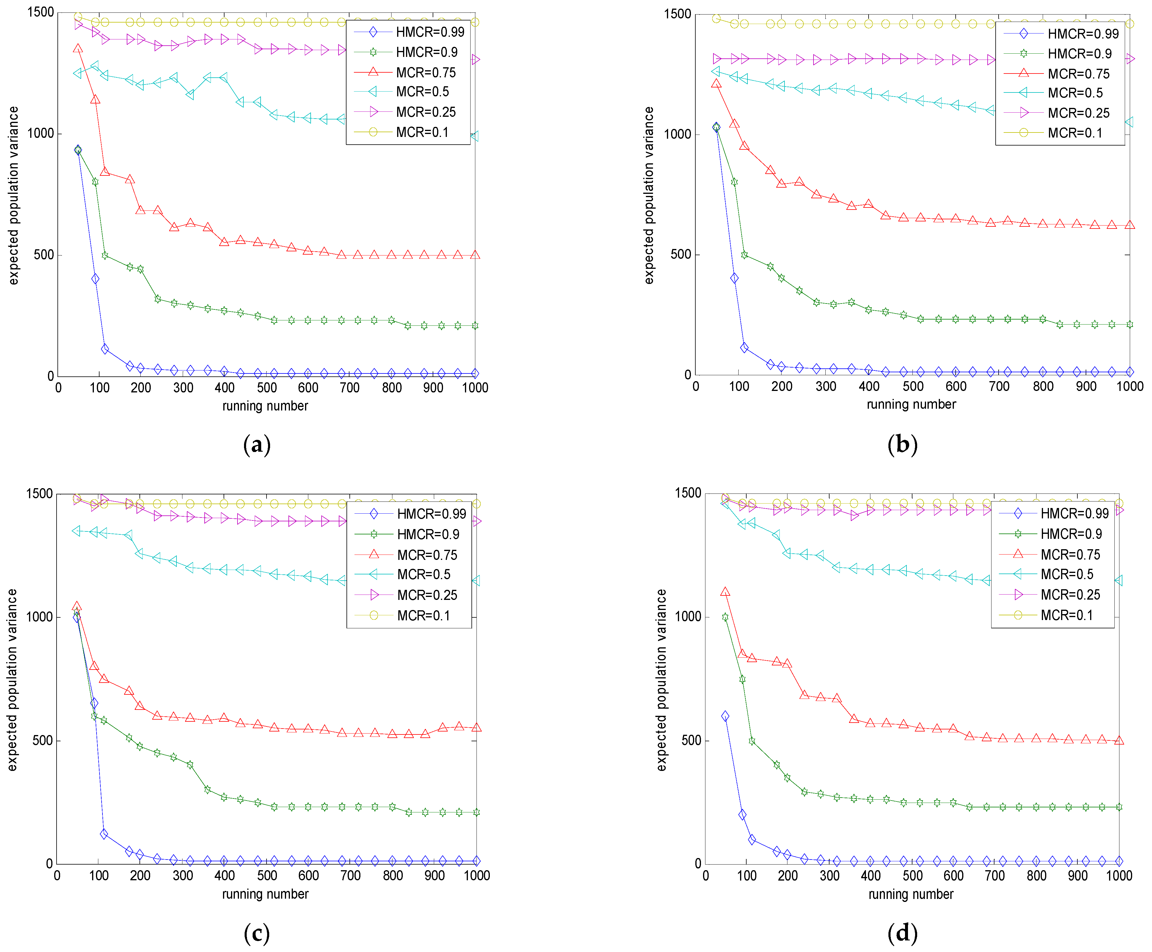
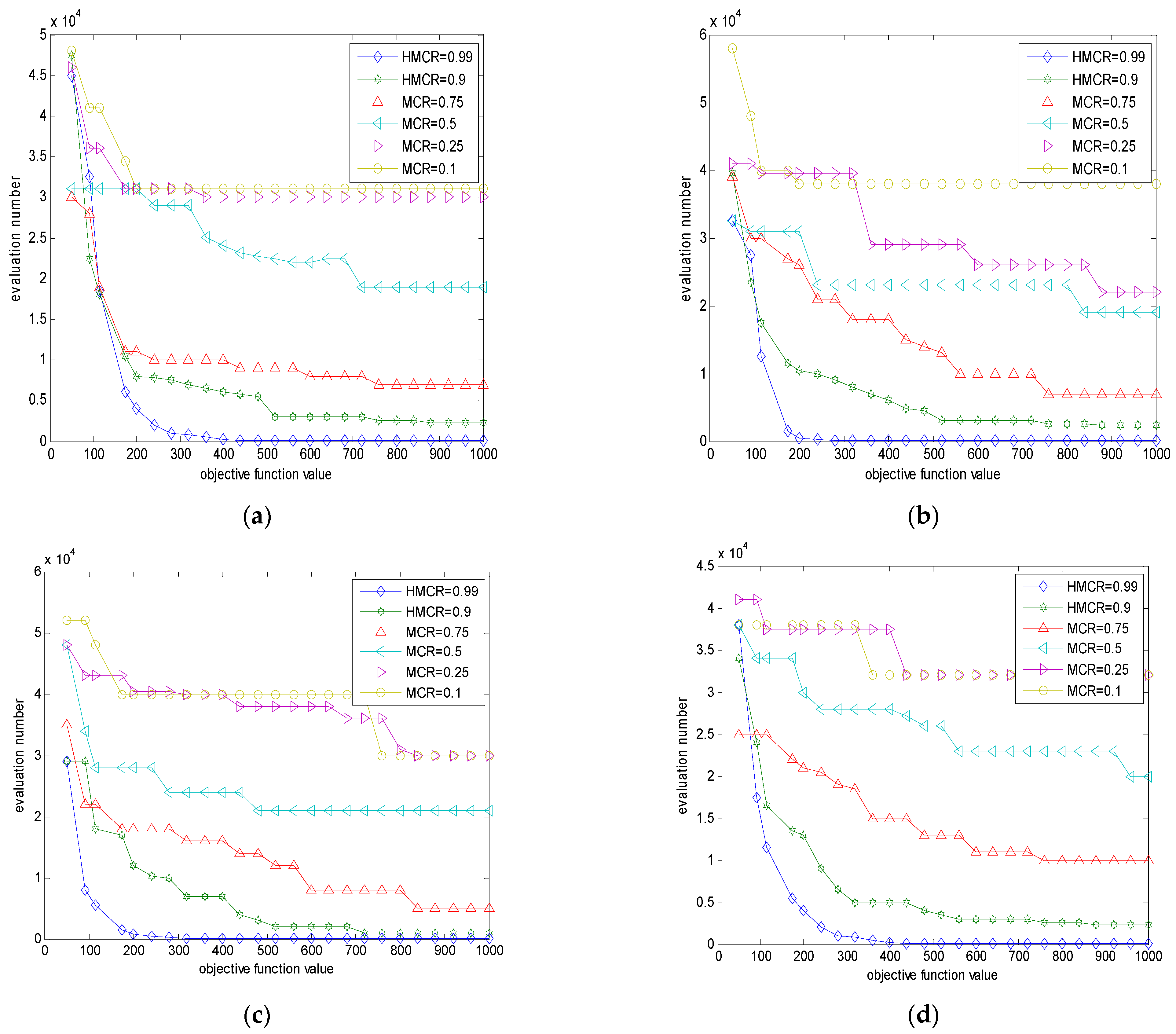
Through the above analysis and discussion, on the one hand, $\mathbf{E}(\mathbf{var}(\mathbf{x}))$, which is related to the original HM initialization, is the part of $\mathbf{E}(\mathbf{var}(\mathbf{y}))$, so it is necessary to find a better initialization method to explore an effective offspring population for improving the algorithm’s exploration. On the other hand, adjusting key control parameters’ values is a good choice to obtain better fine-tuning properties and convergence speed.

The OLPDHS algorithm is proposed. On the one hand, the algorithm improves the initialization method. On the other hand, the fine-tuning properties and convergence speed of HS can be improved by adjusting parameter value. What the OLPDHS algorithm has in common with the classical HS algorithm is that both of them go through four processes: initializing the parameters involved in the algorithm, initializing the harmony memory, improvising a new harmony and updating the harmony memory. The difference between the two is the way of population initialization and the way of control parameter change.

4.1. The Opposite-Based Learning Strategy for Population Initialization

Opposite-based learning (OBL) was first proposed by Tizhooshin in the literature [33]. The main idea of OBL is to obtain a better approximated solution than the current candidate solution, by considering both an estimate and another estimate that is opposite to this estimate, so OBL expands the solution space and reduces the search time [34,35].

Definition 4.

Let$\mathbf{x}=({\mathbf{x}}_1,{\mathbf{x}}_2,···,{\mathbf{x}}_{\mathbf{n}})$be a point in the dimensional$\mathbf{n}$coordinate system, where${\mathbf{x}}_{\mathbf{i}}\in [{\mathbf{a}}_{\mathbf{i}},{\mathbf{b}}_{\mathbf{i}}],\mathbf{i}=1,2,\dots ,\mathbf{n}$, then, the opposite point$\underset{¯}{\mathbf{x}}=({\underset{¯}{\mathbf{x}}}_1,{\underset{¯}{\mathbf{x}}}_2,···,{\underset{¯}{\mathbf{x}}}_{\mathbf{n}})$of$\mathbf{x}$is completely determined according to${\underset{¯}{\mathbf{x}}}_{\mathbf{i}}={\mathbf{a}}_{\mathbf{i}}+{\mathbf{b}}_{\mathbf{i}}-{\mathbf{x}}_{\mathbf{i}}$.

In the original HS algorithm, the initial population is generated in a random way. In order to improve the quality of the initial harmonic memory warehouse, this paper proposes a variety of alternative opposite learning strategies, which include five methods based on opposite learning strategies [36]. Method 1: ${\underset{¯}{\mathbf{x}}}_{\mathbf{i}} = -{\mathbf{x}}_{\mathbf{i}}$, Method 2: ${\underset{¯}{\mathbf{x}}}_{\mathbf{i}}= {\mathbf{a}}_{\mathbf{i}}+{\mathbf{b}}_{\mathbf{i}}-{\mathbf{x}}_{\mathbf{i}}$, Method 3: ${\underset{¯}{\mathbf{x}}}_{\mathbf{i}} = (1/2)\cdot ({\mathbf{a}}_{\mathbf{i}}+{\mathbf{b}}_{\mathbf{i}}-{\mathbf{x}}_{\mathbf{i}})$, Method 4: ${\underset{¯}{\mathbf{x}}}_{\mathbf{i}}=(2\cdot \mathbf{rand}-1)\cdot ( {\mathbf{a}}_{\mathbf{i}}+{\mathbf{b}}_{\mathbf{i}}-{\mathbf{x}}_{\mathbf{i}})$, Method 5: ${\underset{¯}{\mathbf{x}}}_{\mathbf{i}}=\mathbf{rand}( {\mathbf{a}}_{\mathbf{i}}+{\mathbf{b}}_{\mathbf{i}})-{\mathbf{x}}_{\mathbf{i}}$.

4.2. Parameter Adjustment Policy

In order to balance the exploration ability and development ability of the HS algorithm, it is necessary to adjust the key control parameter $\mathbf{b}\mathbf{w}$ dynamically during the search process.

According to Theorem 2, the parameter $\mathbf{b}\mathbf{w}$ ($\mathbf{b}{\mathbf{w}}_{\mathbf{j}}=\sqrt{\gamma \cdot \mathbf{E}(\overline{\mathbf{x}})},$$\overline{\mathbf{x}}=\left(1/\mathbf{HMS}\right){\displaystyle {\sum }_{\mathbf{i}=1}^{\mathbf{HMS}}{\mathbf{x}}_{\mathbf{i}}}$) is dynamically adjusted as follows. To better detail $\mathbf{b}\mathbf{w}$, the more general expression for the average $\mathbf{x}$ of the group is given as Equation (40):

$$\overline{{\mathbf{x}}_{\mathbf{j}}}=\left(1/\mathbf{HMS}\right){\displaystyle {\sum }_{\mathbf{l}=1}^{\mathbf{HMS}}{\mathbf{x}}_{\mathbf{l},\mathbf{j}}},\hspace{0.33em}\mathbf{j}=1,2,···,\mathbf{D},$$

(40)

where $\mathbf{j}$ is the $\mathbf{j}$th dimension of the problem, $\mathbf{D}$ is the maximum dimension of the problem and $\overline{{\mathbf{x}}_{\mathbf{j}}}$ represents the average value of the $\mathbf{j}$th dimension variable. Then, get $\mathbf{E}(\overline{{\mathbf{x}}_{\mathbf{j}}})=\frac{1}{\mathbf{HMS}}{\displaystyle \sum _{\mathbf{l}=1}^{\mathbf{HMS}}\mathbf{E}({\mathbf{x}}_{\mathbf{l},\mathbf{j}})}=\mathbf{E}({\mathbf{x}}_{\mathbf{r},\mathbf{j}})$, here ${\mathbf{x}}_{\mathbf{r},\mathbf{j}}$ are randomly selected from HM and $\mathbf{P}(\mathbf{r}=\mathbf{w})=\frac{1}{\mathbf{HMS}}$, thus $\mathbf{E}({\mathbf{x}}_{\mathbf{r},\mathbf{j}})$ can be obtained as Equation (41).

$$\mathbf{E}({\mathbf{x}}_{\mathbf{r},\mathbf{j}})={\displaystyle \sum _{\mathbf{w}=1}^{\mathbf{HMS}}{\mathbf{p}}_{\mathbf{w}}\cdot {\mathbf{x}}_{\mathbf{w},\mathbf{j}}}={\displaystyle \sum _{\mathbf{w}=1}^{\mathbf{HMS}}\mathbf{p}(\mathbf{r}=\mathbf{w})\cdot {\mathbf{x}}_{\mathbf{w},\mathbf{j}}}=\frac{1}{\mathbf{HMS}}{\displaystyle \sum _{\mathbf{w}=1}^{\mathbf{HMS}}{\mathbf{x}}_{\mathbf{w},\mathbf{j}}}=\overline{{\mathbf{x}}_{\mathbf{j}}},$$

(41)

Thus the result of the parameter $\mathbf{b}\mathbf{w}$ is obtained.

$$\mathbf{b}{\mathbf{w}}_{\mathbf{j}}=\sqrt{\gamma \cdot \overline{{\mathbf{x}}_{\mathbf{j}}}},$$

(42)

It can be seen from Equation (42) that the dynamic adjustment of the parameter $\mathbf{b}\mathbf{w}$ mainly depends on the square root of the mean value of the harmony vectors of the population after each update. In this way, it is easier to realize the actual operation of dynamic adjustment of the parameter $\mathbf{b}\mathbf{w}$. When the new solution is fine-tuned according to Equation (40) or Equation (41), the information of the current population is carried out by the parameter $\mathbf{b}\mathbf{w}$. The fine-tuning of the new solution has global guiding significance. However, the fine-tuning solution with the fixed value of the parameter $\mathbf{b}\mathbf{w}$ does not consider the current population search situation. Additional calculation $\mathbf{E}\left(\overline{{\mathbf{x}}_{\mathbf{j}}}\right)$ after each evolution is required, which increases the calculation amount of the algorithm.

5. Simulation Experiments and Analysis of OLPDHS

In order to verify the rationality and effectiveness of the OLPDHS algorithm in this paper, MATLAB is used to test algorithm performance from different perspectives.

5.1. Influence of the Parameters HMCR, HMS and PAR on OLPDHS

Firstly, the influence of the parameter HMCR on the performance of the OLPDHS algorithm is analyzed by simulation. The unimodal function Sphere and the multimodal function Rastrigin are used as the test functions, and the parameters are set as HMS = 5, PAR = 0.5, $\mathbf{b}{\mathbf{w}}_{\mathbf{j}}=\sqrt{\gamma \cdot \mathbf{E}(\overline{\mathbf{x}})}$, $\gamma =\mathbf{E}(\overline{\mathbf{x}})$, the maximum number of evolutions $G=1000$, the dimension of the function is 30, and the HMCR is changed dynamically from 0.1 to 0.99, proceeding through 0.1, 0.25, 0.5, 0.75, 0.9 and 0.99. MATLAB is used for simulation, and the relationship between the population variance expectation and the iterations number is obtained, as shown in Figure 2. It reflects that for the function Sphere and the function Rastrigin, when the values of parameter HMCR are different, the search capability of the OLPDHS algorithm changes over iterations. Figure 3 shows the relation between the Sphere function value and the Rastrigin function value obtained by the OLPDHS algorithm under different parameter HMCR values with the change of evaluation numbers, reflecting the influence of different parameter HMCR values on the convergence performance of the OLPDHS algorithm.

As can be seen from Figure 2 and Figure 3, the value of HMCR has a great impact on the expected population variance and the convergence of the OLPDHS algorithm. With the increase in the value of HMCR, the smaller the expected population variance and convergence accuracy, the larger the value of HMCR and the better the convergence rate of the OLPDHS algorithm.

In addition, when HMCR values are 0.01, 0.25, 0.5, 0.75, 0.9, 0.95, and 0.99, the mean value and variance results of the two test functions are shown in

Table 1. Numerical results with different HMCR values for Sphere.

Initial Range	Index	HMCR
		0.01	0.25	0.5	0.75	0.9	0.95	0.99
[−50, 100]	mean	2.3614 × 104	1.5993 × 104	8.3985 × 103	5.7084 × 102	2.5158 × 10−25	0	0
	SD	1.8327 × 103	2.5753 × 103	1.3622 × 103	1.6108 × 102	5.2121 × 10−25	0	0
[−100, 50]	mean	2.3294 × 104	1.6440 × 104	8.3378 × 103	5.4782 × 102	1.1731 × 10−25	0	0
	SD	2.4008 × 103	1.5064 × 103	1.3824 × 103	2.0766 × 102	3.0618 × 10−25	0	0

and

Table 2. Numerical results with different HMCR values for Rastrigin.

Initial Range	Index	HMCR
		0.01	0.25	0.5	0.75	0.9	0.95	0.99
[−50, 100]	mean	2.4092 × 104	1.7223 × 104	8.8618 × 103	8.6880 × 102	3.8905	0	0
	SD	2.3756 × 103	1.2709 × 103	1.3189 × 103	2.0211 × 102	7.2482	0	0
[−100, 50]	mean	2.4289 × 104	1.6280 × 104	8.7667 × 103	7.9659 × 102	4.6300	0	0
	SD	2.2072 × 103	1.9277 × 103	1.1763 × 103	2.0847 × 102	1.3894 × 10−1	0	0

, respectively. For the Sphere function, Table 1 shows that the smaller the value of HMCR, the worse the performance of the OLPDHS algorithm. When HMCR < 0.9, the results obtained by the OLPDHS algorithm have deviated significantly from the global optimal solution. When HMCR > 0.9, the OLPDHS algorithm quickly converges to or near the global optimal solution. For the multimodal function Rastrigin, Table 2 shows that the value of HMCR has a similar impact on the performance of the OLPDHS algorithm to that in the Sphere function. According to Table 1 and Table 2, the convergence accuracy is better with the increase in HMCR value.

Then, the influence of parameter HMS and parameter PAR on the OLPDHS algorithm is analyzed through simulation experiments. Nine functions ($f_1\sim f_9$) with different characteristics are selected to study the impact of parameters HMS and PAR on the performance of the OLPDHS.

$$\begin{array}{l}{f}_1={\displaystyle {\sum }_{\mathbf{i}=1}^{\mathbf{D}}{\mathbf{x}}_{\mathbf{i}}^2},\hspace{0.33em}{\mathbf{x}}_{\mathbf{i}}\in [-100,100],\hspace{0.33em}{f}_{\mathbf{min}}=0\\ f_2={\displaystyle {\sum }_{\mathbf{i}=1}^{\mathbf{D}}‖{\mathbf{x}}_{\mathbf{i}}‖}+{\displaystyle {\prod }_{\mathbf{i}=1}^{\mathbf{D}}‖{\mathbf{x}}_{\mathbf{i}}‖},\hspace{0.33em}{\mathbf{x}}_{\mathbf{i}}\in [-100,100],\hspace{0.33em}{f}_{\mathbf{min}}=0\\ f_3={\displaystyle {\sum }_{\mathbf{i}=1}^{\mathbf{D}}{({\displaystyle {\sum }_{\mathbf{j}=1}^{\mathbf{i}}{\mathbf{x}}_{\mathbf{j}}})}^2},\hspace{0.33em}{\mathbf{x}}_{\mathbf{i}}\in [-100,100],\hspace{0.33em}{f}_{\mathbf{min}}=0\\ f_4={\displaystyle {\sum }_{\mathbf{i}=1}^{\mathbf{D}}-{\mathbf{x}}_{\mathbf{i}}}\times \mathbf{sin}\sqrt{‖{\mathbf{x}}_{\mathbf{i}}‖},\hspace{0.33em}{\mathbf{x}}_{\mathbf{i}}\in [-500,500],\hspace{0.33em}{f}_{\mathbf{min}}=-418.9829\mathrm{D}\\ f_5={\displaystyle {\sum }_{\mathbf{i}=1}^{\mathbf{D}}[{\mathbf{x}}_{\mathbf{i}}^2-10\mathbf{cos}(2\prod {\mathbf{x}}_{\mathbf{i}})+10]},\hspace{0.33em}{\mathbf{x}}_{\mathbf{i}}\in [-5.12,5.12],\hspace{0.33em}{f}_{\mathbf{min}}=0\\ f_6=(1/4000){\displaystyle {\sum }_{\mathbf{i}=1}^{\mathbf{D}}{\mathbf{x}}_{\mathbf{i}}^2}-{\displaystyle {\prod }_{\mathbf{i}=1}^{\mathbf{D}}\mathbf{cos}({\mathbf{x}}_{\mathbf{i}}/\sqrt{\mathbf{i}})}+1,\hspace{0.33em}{\mathbf{x}}_{\mathbf{i}}\in [-600,600],\hspace{0.33em}{f}_{\mathbf{min}}=0\\ f_7=1/4({\mathbf{x}}_{\mathbf{i}}+1)+1,\hspace{0.33em}{\mathbf{x}}_{\mathbf{i}}\in [-50,50],\hspace{0.33em}{f}_{\mathbf{min}}=0\\ f_8={\displaystyle {\sum }_{\mathbf{i}=1}^{\mathbf{n}-1}[{({\mathbf{x}}_{\mathbf{i}}^2+{\mathbf{x}}_{\mathbf{i}+1}^2)}^{0.25}(\mathbf{sin}{(50({\mathbf{x}}_{\mathbf{i}}^2+{\mathbf{x}}_{\mathbf{i}+1}^2{)}^{0.1})}^2+1)]},\hspace{0.33em}{\mathbf{x}}_{\mathbf{i}}\in [-100,100],\hspace{0.33em}{f}_{\mathbf{min}}=0\\ f_9={\displaystyle {\sum }_{\mathrm{i}=1}^2{\mathbf{x}}_{\mathbf{i}}^2}+{({\displaystyle {\sum }_{\mathrm{i}=1}^{2}0.5\mathbf{i}{\mathbf{x}}_{\mathbf{i}}})}^2+{({\displaystyle {\sum }_{\mathrm{i}=1}^{2}0.5\mathbf{i}{\mathbf{x}}_{\mathbf{i}}})}^4,\hspace{0.33em}{\mathbf{x}}_{\mathbf{i}}\in [-100,100],\hspace{0.33em}{f}_{\mathbf{min}}=0\end{array}$$

The dimension of all functions is set to 30, the maximum number of iterations to 20,000, and each function is set to run 30 times independently.

Table 3. Effects of PAR for nine functions.

PAR	Index	${\mathit{f}}_1(\mathbf{x})$	${\mathit{f}}_2(\mathbf{x})$	${\mathit{f}}_3(\mathbf{x})$	${\mathit{f}}_4(\mathbf{x})$	${\mathit{f}}_5(\mathbf{x})$	${\mathit{f}}_6(\mathbf{x})$	${\mathit{f}}_7(\mathbf{x})$	${\mathit{f}}_8(\mathbf{x})$	${\mathit{f}}_9(\mathbf{x})$
0.1	mean	7.96 × 10−90	1.48 × 10−53	685.9444	−12362.6	0	0.009833	0.007098	9.87 × 10−26	21,204.57
	SD	4.11 × 10−89	7.89 × 10−53	514.0565	128.0777	0	0.002543	0.019818	2.16 × 10−25	8073.396
0.2	mean	9 × 10−164	2.1 × 10−105	0.081202	−9558.07	0	0.007004	0.059908	6.97 × 10−55	1182.936
	SD	0	8.8 × 10−105	0.424572	466.2021	0	0.000739	0.044512	7.96 × 10−55	2167.133
0.3	mean	1.5 × 10−182	1.4 × 10−119	0.002347	−7993.01	0	0.002974	0.072704	3.56 × 10−62	779.3931
	SD	0	3.2 × 10−119	0.012182	450.3964	0	0	0.041652	5.33 × 10−62	1491.498
0.4	mean	1.2 × 10−188	3.2 × 10−124	1.14× 10−5	−6934.18	0	0	0.082485	2 × 10−65	370.6182
	SD	0	1.7 × 10−123	2.87× 10−5	480.1842	0	0.000247	0.030938	4.27 × 10−65	509.1225
0.5	mean	3 × 10−192	7.1 × 10−127	1.61× 10−5	−6077.32	0	0.00135	0.106701	7.54 × 10−66	390.7553
	SD	0	2.8 × 10−126	5.2× 10−5	437.4262	0	0	0.04902	3.13 × 10−65	665.9627
0.6	mean	2.2 × 10−191	1.2 × 10−128	0.000421	−5464.39	0	0	0.115062	6.85 × 10−66	896.9894
	SD	0	3.3 × 10−128	0.001731	328.2753	0	0	0.042131	1.53 × 10−65	1310.2
0.7	mean	2.3 × 10−189	4.9 × 10−127	4.04× 10−5	−4854.59	5.92 × 10−17	0	0.120986	3.16 × 10−65	401.8195
	SD	0	1.5 × 10−126	9.66× 10−5	419.4351	3.24 × 10−16	0.001129	0.034338	1.22 × 10−64	674.5876
0.8	mean	1.1 × 10−184	4.5 × 10−122	0.00303	−4374.65	0	0.006181	0.148274	8.87 × 10−64	1071.784
	SD	0	2.4 × 10−121	0.01554	254.9838	0	0.002133	0.045609	2.22 × 10−63	1331.394
0.9	mean	1.2 × 10−175	5.1 × 10−118	0.05821	−3583.87	1.67668	0.011683	0.170418	7.77 × 10−61	834.9668
	SD	0	1.4 × 10−117	0.261077	306.3736	5.133747	0.009833	0.047123	2.79 × 10−60	1154.953
1	mean	6.7 × 10−171	3.8 × 10−119	0.004582	−3597.4	0	0.002543	0.167839	1.8 × 10−60	782.5468
	SD	0	7.8 × 10−119	0.013117	327.2936	0	0.007004	0.035659	2.55 × 10−60	1028.296

lists the mean value and standard deviation (SD) value of each function while running 30 times independently under different values of parameter PAR.

Table 4. Effects of HMS for nine functions.

HMS	Index	${\mathit{f}}_1(\mathbf{x})$	${\mathit{f}}_2(\mathbf{x})$	${\mathit{f}}_3(\mathbf{x})$	${\mathit{f}}_4(\mathbf{x})$	${\mathit{f}}_5(\mathbf{x})$	${\mathit{f}}_6(\mathbf{x})$	${\mathit{f}}_7(\mathbf{x})$	${\mathit{f}}_8(\mathbf{x})$	${\mathit{f}}_9(\mathbf{x})$
5	mean	1.2 × 10−182	2.7 × 10−122	0.000169	−7566.71	5.92 × 10−17	0.00074	0.061816	9.72 × 10−64	277.7771
	SD	0	9.5 × 10−122	0.000665	479.2929	3.24 × 10−16	0.002257	0.025266	3.22 × 10−63	405.6994
10	mean	1.01 × 10−98	8.34 × 10−65	9.380667	−8360.2	5.33 × 10−16	0.000821	0.027107	1.45 × 10−31	12,398.39
	SD	3.83 × 10−98	1.06 × 10−64	14.24209	374.3772	2.92 × 10−15	0.003125	0.007286	2.92 × 10−31	6517.15
20	mean	1.19 × 10−51	8.68 × 10−34	748.1719	−8909.59	6.045465	0.001397	0.014194	2.34 × 10−15	39,830.05
	SD	0	1.42 × 10−33	683.1214	363.7991	9.443056	0.003281	0.005153	3 × 10−15	987.6950
40	mean	1.2 × 10-188	1.43 × 10−17	4649.907	−9324.05	21.20932	0.001137	0.012963	2.98 × 10−7	55,213.7
	SD	0	1.24 × 10-17	3231.415	290.8353	15.59811	0.003059	0.005449	1.46 × 10−7	9326.81
80	mean	3 × 10-192	7.41 × 10−9	10,348.01	−9573.82	26.70999	0.00097	0.01582	0.011469	59,363.13
	SD	0	2.61 × 10−9	3197.345	322.8402	9.894514	0.002516	0.003128	0.003728	9059.778
100	mean	2.2 × 10−191	5.67 × 10−7	13,876.19	−9370.6	30.70935	0.000403	0.018056	0.062568	59,859.2
	SD	0	2.7 × 10−7	3547.672	344.3145	10.11926	0.001584	0.003564	0.019463	5685.164
120	mean	2.3 × 10−189	1.12 × 10−5	15,843.26	−9388.53	36.75415	0.000967	0.021201	0.181106	61,586.09
	SD	0	3.52 × 10−6	4620.502	254.8811	13.51672	0.00369	0.005331	0.029841	7329.876
150	mean	1.1 × 10−184	0.000215	18,886.69	−9287.02	39.57804	0.000523	0.02599	0.622355	61,045.64
	SD	0	5.96 × 10−5	4051	368.5464	12.15133	0.002706	0.004039	0.117255	6132.338
200	mean	1.2 × 10−175	0.004857	25,336.71	−9019.63	41.69105	0.004459	0.038315	2.236501	58,995.2
	SD	0	0.000922	3946.534	349.0453	10.18421	0.001887	0.007615	0.391213	5730.374
500	mean	6.7 × 10−171	1.996803	34,581.73	−8362.23	54.67448	1.202493	5.468026	29.92783	60,399.91
	SD	0	0.255739	4976.491	309.6179	8.477906	0.028179	1.426998	2.088327	6872.494

shows the mean value and SD value of each function while running 30 times independently under different values of parameter HMS. Figure 4 and Figure 5 visually show the optimization curves of nine functions under different values of parameters HMS and PAR.

As observed in Table 3, none of the PAR values performs well for all of the test functions. When the value of PAR is in the interval [0.3, 0.7], the mean and SD of all the functions except function $f_4$ and function $f_7$ are relatively good. For function $f_4$, the larger value of parameter PAR results in poor performance of the OLPDHS algorithm. For function $f_7$, the values of PAR have little effect on the performance of the OLPDHS algorithm. By observing Figure 4 and comparing the optimization curves, it can be found that when PAR is in the interval [0.3, 0.7], the optimization curves of the OLPDHS algorithm are better. Thus, the value of PAR has an impact on the performance of the OLPDHS algorithm, and the value is determined based on the analysis of the specific optimization problem.

As can be seen from Table 4, except for the function $f_4$ (when the HMS value is large, the optimization result is better), the convergence accuracy of other functions deteriorates as the HMS value increases. As shown in Figure 5, except for function $f_4$, the optimization curve obtained by other functions is better with the decrease in HMS value. Through analysis, it can be concluded that the value of HMS is appropriate in the interval [5, 40].

Finally, the parameter value range of the OLPDHS algorithm to obtain better performance can be obtained through the above simulation analysis. The specific values of parameters should be determined by the optimization problem itself and the optimization model, which must be tested repeatedly in practice.

5.2. Performance Comparison of the OLPDHS Algorithm and Other HS Algorithms

In order to prove the efficiency of the OLPDHS algorithm, the OLPDHS algorithm is compared with the recently developed HS algorithm and its improved version (IHS [37], GHS [38], SAHS [39], SGHS [40], NGHS [41] NDHS [42], EHS [30] and ITHS [43]) by testing the unconstrained optimization problem. Related parameters are set as follows: (1) $\mathbf{HMCR}$: SGHS is 0.98, NDHS, EHS, and ITHS are 0.99, OLPDHS is 0.9999, and other algorithms are 0.9; (2) $\mathbf{HMS}$: the value is 50 for EHS, 10 for ITHS and 5 for other algorithms; (3) $\mathbf{PAR}$: HS and EHS are set to 0.33, GHS, IHS and OLPDHS are set to 0.1 and 0.99, SAHS and ITHS are set to 0 and 1, NDHS is set to 0.01, 0.99 and SGHS is set to 0.9; (4) $\mathbf{b}\mathbf{w}$: HS is 0.01, SGHS is 0.0005 and $({\mathbf{x}}^{\mathbf{U}}-{\mathbf{x}}^{\mathbf{L}})/20$, IHS is 0.0001 and $({\mathbf{x}}^{\mathbf{U}}-{\mathbf{x}}^{\mathbf{L}})/20$, and EHS is $1.17\sqrt{\mathbf{x}\left(\mathbf{var}\right)}$; In addition, ${\mathbf{p}}_{\mathbf{m}}=2/\mathbf{N}$ in NGHS. Among the nine functions, $f_1$,$f_2$,$f_3$ are single peak functions; $f_5$,$f_6$,$f_7$ are multi-peak functions, and with the increase in the dimension of the problem, the number of locally optimal solutions increases. The functions $f_8$ and $f_9$ are low-dimensional functions, which have more local optimal solutions.

Figure 6 shows the convergence properties of 10 algorithms tested by 9 functions with 30 dimensions. In most cases, the OLPDHS algorithm has better convergence than the other nine HS algorithms. Except for functions $f_4$ and $f_7$, the convergence of the OLPDHS algorithm is not as good as expected, while SGHS, NGHS and EHS algorithms have a better convergence trend. For functions $f_3$ and $f_9$, the OLPDHS algorithm has a convergence no better than the ITHS algorithm, but the OLPDHS algorithm has better performance than other algorithms. On the whole, the OLPDHS algorithm has faster convergence than other HS algorithms.

6. Task-Allocation Simulation Experiment Based on OLPDHS

In order to fully verify the effectiveness of the task-allocation algorithm and model designed in this paper, three unmanned aerial vehicles with different loads were used to perform eight different mission objectives as a combat example for simulation verification. In the simulation, four algorithms are used to independently solve the task assignment model 10 times, respectively. The simulation environment and algorithm parameters are consistent with the Section 5.

6.1. Initial Information of Simulation

Battlefield space is a 100 km × 100 km square map. According to the description of the modeling process in Section 2, the terrain-steepness factor is $\lambda =1.5$, track weight and loss weight are ${\mathsf{\omega }}_1=0.5, {\mathsf{\omega }}_2=0.5$ and the penalty factor of the constraint term is δ = 5. At the same time, the maximum number of tasks that each UAV can perform is set to $\mathbf{Loa}{\mathbf{d}}_{\mathbf{i}}=3$, where $\mathbf{i}$ represents the number of UAVs. The maximum range of the UAVs is set to $\mathbf{D}{\left(\mathbf{i}\right)}_{\mathbf{max}}=600 \mathrm{km}$. According to the task-allocation code in Section 2.5, the dimension of the allocation model is set to the task target number $\mathbf{dim}=8$, the scope of individual search is (0,3), the number of individuals in each algorithm is set to 10, and the iteration number is 1000. The heterogeneity of multiple UAV formations with different loads is directly reflected by the capability value of performing a specific task. The specific parameters of UAVs and mission targets are shown in

Table 5. Performance parameters of three UAVs.

Number of UAV	Worth	Position (km)	Defense	Target Capacity	$\mathbf{P}(\mathbf{T})$
1	0.9	(10,20)	0.3	reconnaissance	0.9
				attack	0.2
				evaluation	0.8
2	0.7	(30,10)	0.9	reconnaissance	0.3
				attack	0.9
				evaluation	0.4
3	0.8	(15,9)	0.5	reconnaissance	0.5
				attack	0.5
				evaluation	0.5

and

Table 6. Parameters of eight mission objectives.

Number of Mission	Type	Worth	Position (km)	Defense	Strike
T1	m1	0.4	(80,50)	0.2	0.8
T2	m3	0.5	(60,45)	0.4	0.6
T3	m3	0.9	(80,80)	0.9	0.1
T4	m2	0.8	(90,20)	0.7	0.3
T5	m2	0.9	(50,90)	0.8	0.2
T6	m3	0.5	(60,65)	0.4	0.6
T7	m2	0.7	(40,90)	0.7	0.3
T8	m1	0.6	(70,45)	0.2	0.8

.

In order to visually display the battlefield environment and task-assignment process, this paper draws the battlefield environment through Visio 2017 software, as shown in Figure 7 below.

6.2. Simulation and Analysis

Four intelligent algorithms are used to independently solve the task-allocation model 10 times. The solution results are shown in

Table 7. The results of 10 times obtained independently by two algorithms.

Algorithm	Tar-Fitness-Final	Time Cost	P	Algorithm	Tar-Fitness-Final	Time Cost	P
OLPDHS	1.5449	0.0809	100%	SAHS	1.4755	0.0635	100%
	1.5268	0.0817			1.4381	0.0609
	1.5491	0.0824			1.4829	0.0620
	1.5491	0.0902			1.4733	0.0593
	1.5491	0.0782			1.4733	0.0604
	1.5238	0.0810			1.4723	0.0603
	1.5231	0.0808			1.4486	0.0623
	1.5491	0.0825			1.4435	0.0616
	1.5491	0.0799			1.4413	0.0625
	1.5238	0.0817			1.4805	0.0627
Mean	1.5388	0.0819	-	Mean	1.4629	0.0616	-
Algorithm	Tar-Fitness-Final	Time Cost	P	Algorithm	Tar-Fitness-Final	Time Cost	P
NDHS	1.5263	0.0855	100%	NGHS	1.5449	0.0786	100%
	1.5491	0.0893			1.5102	0.0782
	1.4831	0.0857			1.4875	0.0805
	1.5449	0.0890			1.4831	0.0843
	1.5280	0.0873			1.4755	0.0798
	1.5491	0.0864			1.4755	0.0775
	1.5028	0.0913			1.4682	0.0774
	1.4942	0.0885			1.4682	0.0766
	1.4926	0.0885			1.4527	0.0789
	1.4834	0.0883			1.4397	0.0825
Mean	1.5154	0.0880	-	Mean	1.4806	0.0794	-

, where $\mathbf{Tar}\_\mathbf{fitness}\_\mathbf{final}$ represents the final task fitness; the higher the fitness, the better the feasible solution iterated by the algorithm. $\mathbf{P}$ represents the success rate of the algorithm solution, and $\mathbf{Mean}$ is the average of the solution results obtained 10 times for each algorithm.

Further analysis of Table 7 shows that the solving success rate of each algorithm is 100%, which verifies the effectiveness of the multi-UAV task-allocation model constructed in this paper. Meanwhile, the average fitness of 10 independent solutions of the OLPDHS algorithm is 1.5388, which is higher than the average fitness of the other three algorithms. Therefore, in solving task assignment problems, the optimization algorithm based on improved chaotic adaptive strategies designed in this paper is superior to the other three comparison algorithms. Figure 8 shows the fitness convergence process of four algorithms for solving the task assignment model. It can be seen from the figure that the OLPDHS algorithm can quickly converge to a relatively excellent fitness value in the early stage, and the fitness is higher than the other three algorithms in the late iteration, which further reflects the effectiveness of OLPDHS in solving the task assignment.

In order to directly reflect the time consumption of the two algorithms, the tic and toc functions in MATLAB are used to obtain the time-consumption data in

Table 8. Assignment results of task objectives corresponding to optimal fitness.

Algorithm	Tar_fitness_final	Assignment Results of Task Objectives
OLPDHS	1.5491	UAV1: T8→T1→T4 UAV2: T2→T6 UAV3: T7→T5→T3
SAHS	1.4829	UAV1: T5→T3→T8 UAV2: T2→T1→T4 UAV3: T7→T6
NDHS	1.5491	UAV1: T8→T1→T4 UAV2: T2→T6 UAV3: T7→T5→T3
NGHS	1.5449	UAV1: T8→T1→T3 UAV2: T4→T2 UAV3: T6→T5→T7

. Based on the data in the table, the time-consumption graph of the four algorithms after 10 iterations of independent operation is drawn in Figure 9. It can be seen from the figure that the SAHS algorithm has the lowest time consumption, while the NDHS algorithm has the highest time consumption. Although OLPDHS is more time-consuming, OLPDHS improves the fitness of feasible solutions of the task-allocation model, so the cost of sacrificing some time is acceptable.

Table 8 shows the target allocation results corresponding to the optimal fitness obtained by running four algorithms for 10 times. Meanwhile, the allocation results are drawn on the basis of Figure 7 as shown in Figure 10.

7. Related Work

There are many researchers dedicated to the study of task allocation, and many methods have been put forward. This section mainly summarizes the methods of task allocation in various fields and the achievements achieved in UAV task allocation.

The threshold-based method is used to solve task-allocation problems. In 2005, extreme teams, large-scale agent teams operating in dynamic environments, were on the horizon. Low-communication approximate distributed constraint optimization (LADCOP), a distributed threshold-based algorithm, was proposed to solve task-allocation problems in the domain of simulated disaster rescue. The tasks are perceived by the agents in the environment [44]. In 2007, swarm generalized assignment problem (Swarm-GAP) was used to experiment in the RoboCup rescue simulator [45]. In 2010, considering the various actors in the RoboCup rescue, Swarm-GAP, LADCOP and a greedy method were used to solve distributed task allocation among teams of agents in a RoboCup rescue scenario [46]. The results showed that the performance of Swarm-GAP and LADCOP are similar and that they outperform a greedy strategy. The threshold-based approach is applied to division of labor control for a robot group [47], but the task ordering is performed by a central command unit, which generates a significant number of messages. Swarm-GAP was adopted to deal with this problem and a new method with three algorithm variants was proposed in 2017 [48]. This method effectively prevented some agents from being overloaded with tasks while others remained idle. The aforementioned researchers aimed at the optimization of their resource usage applied in the context of static environments. In 2020, Amorim J C evaluated the performance of three swarm-GAP variants in dynamic contexts, and extended these algorithms to properly address more realistic dynamic scenarios [49].

The market-based method is applied to task-allocation problems. Task specification trees (TSTs) as a highly expressive specification language for complex multiagent tasks were used. Meanwhile, a sound and complete distributed heuristic search algorithm for allocating the individual tasks in a TST to platforms was proposed in 2010 [50]. A decentralized distributed solution approach based on multi-agent systems (MAS) to manage emergency vehicles was developed, and a multi-agent architecture to fit real emergency systems was proposed. A more refined and efficient auction mechanism based on implicit agents’ coordination was examined to coordinate agents to reach good quality solutions in a distributed manner [51]. For the multi-robot dynamic task-allocation problem, multi-objective optimization (MOO) was used to estimate and subsequently make an offer for its assignment. That is, after task detection, an auction took place amongst robots capable of executing it. Robots calculated their bid using MOO [52].

There are also other works that propose methods for allocating tasks. ZORLU [22] considered the UAV load constraints and modeled the problem as a CVRP model with load constraints. Shima T [53] proposed the CMTAP model for UAVs, which divided the task types into identification, attack and damage assessment. The time sequence between tasks, execution time of tasks and multi-UAVs cooperative constraints were added into the model. Min Yao [54] designed a collaborative multi-task assignment model for UAV groups that is suitable for multiple UAVs, multi-task targets and multi-task types. Wen Gu [55] proposed a solution to UAV target allocation problem based on the Hungarian algorithm, and Jin Zhang et al. [56] extended the Hungarian algorithm to multi-target allocation. In addition, [57] used the MILP method to solve multi-UAV target allocation, and other optimization methods include dynamic programming and graph theory.

This current paper considers the type of task, the UAV load constraints, multiple UAVs, multi-task targets and multi-task types, features that are similar to previous studies in the literature [21,53,54]. Unlike these studies, this paper builds a model from two aspects of the rewards and costs of performing tasks.

8. Conclusions

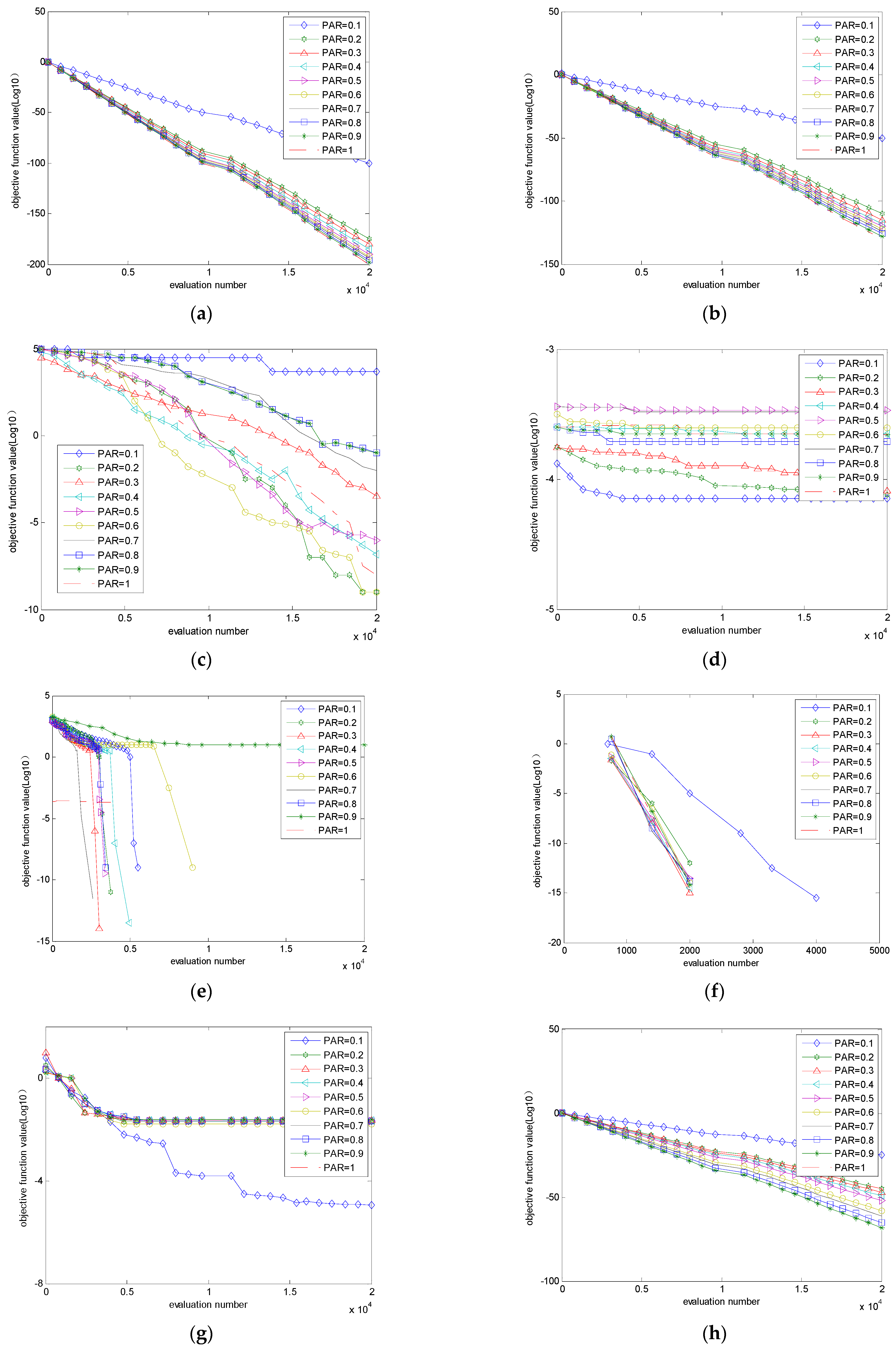
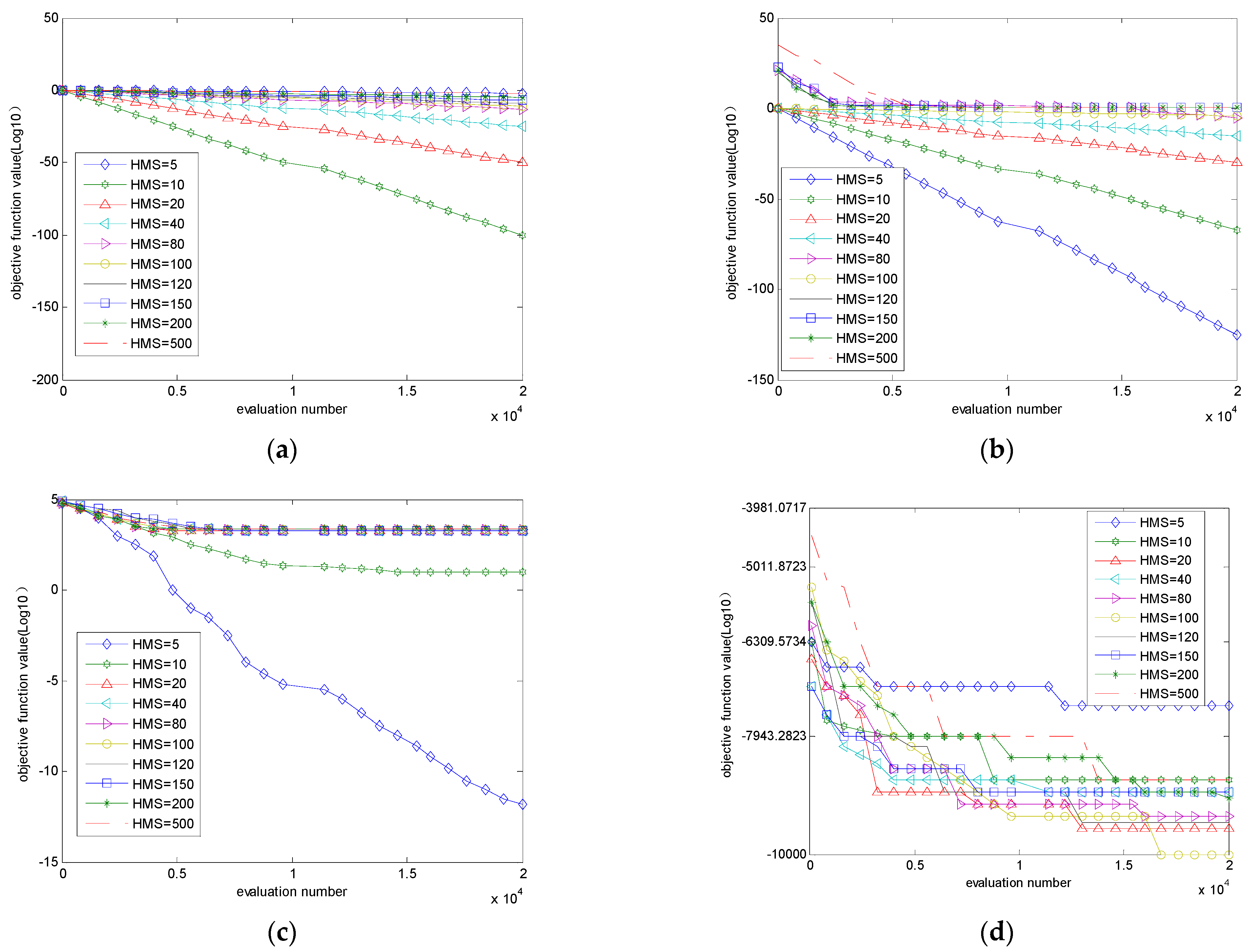
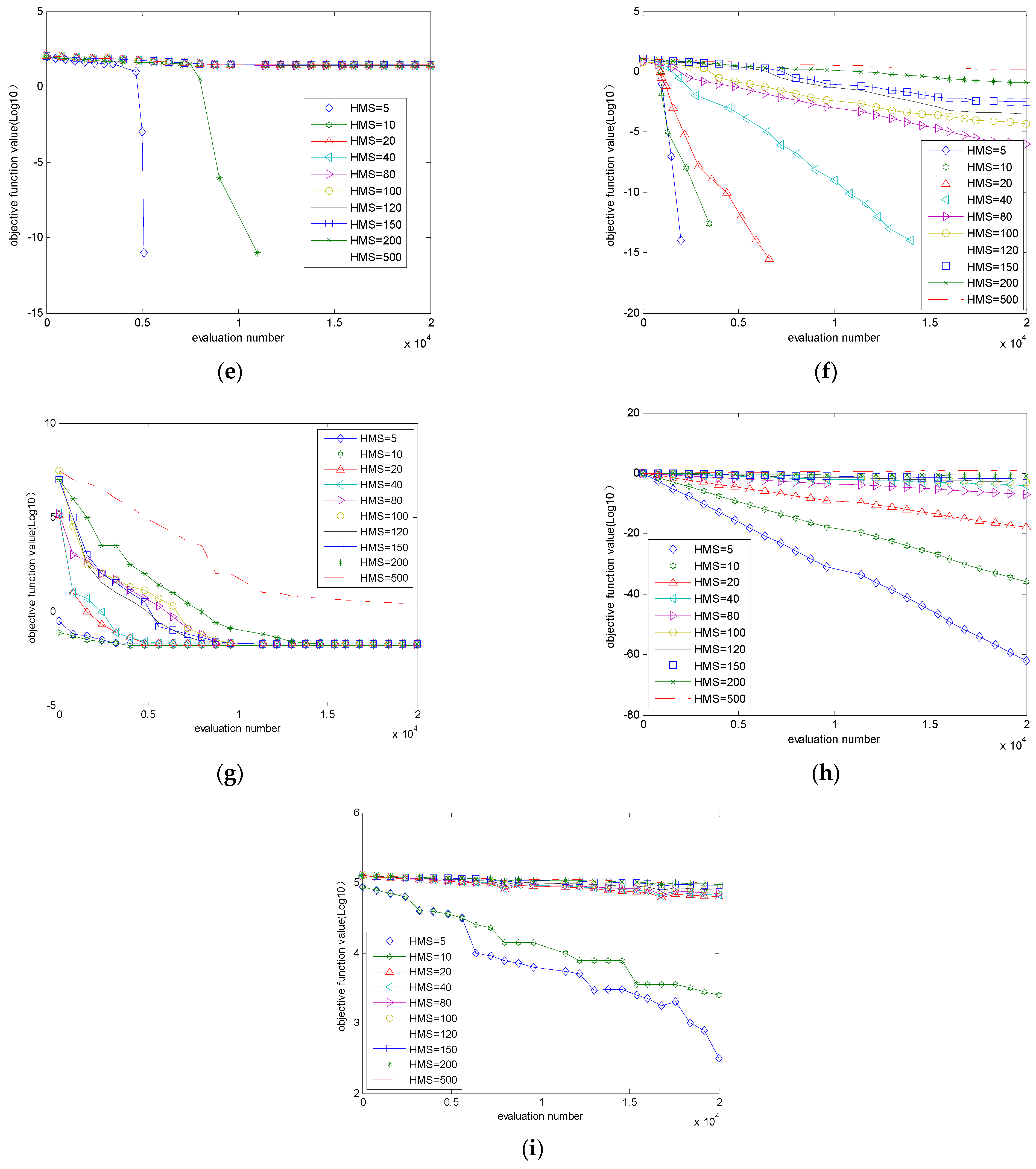
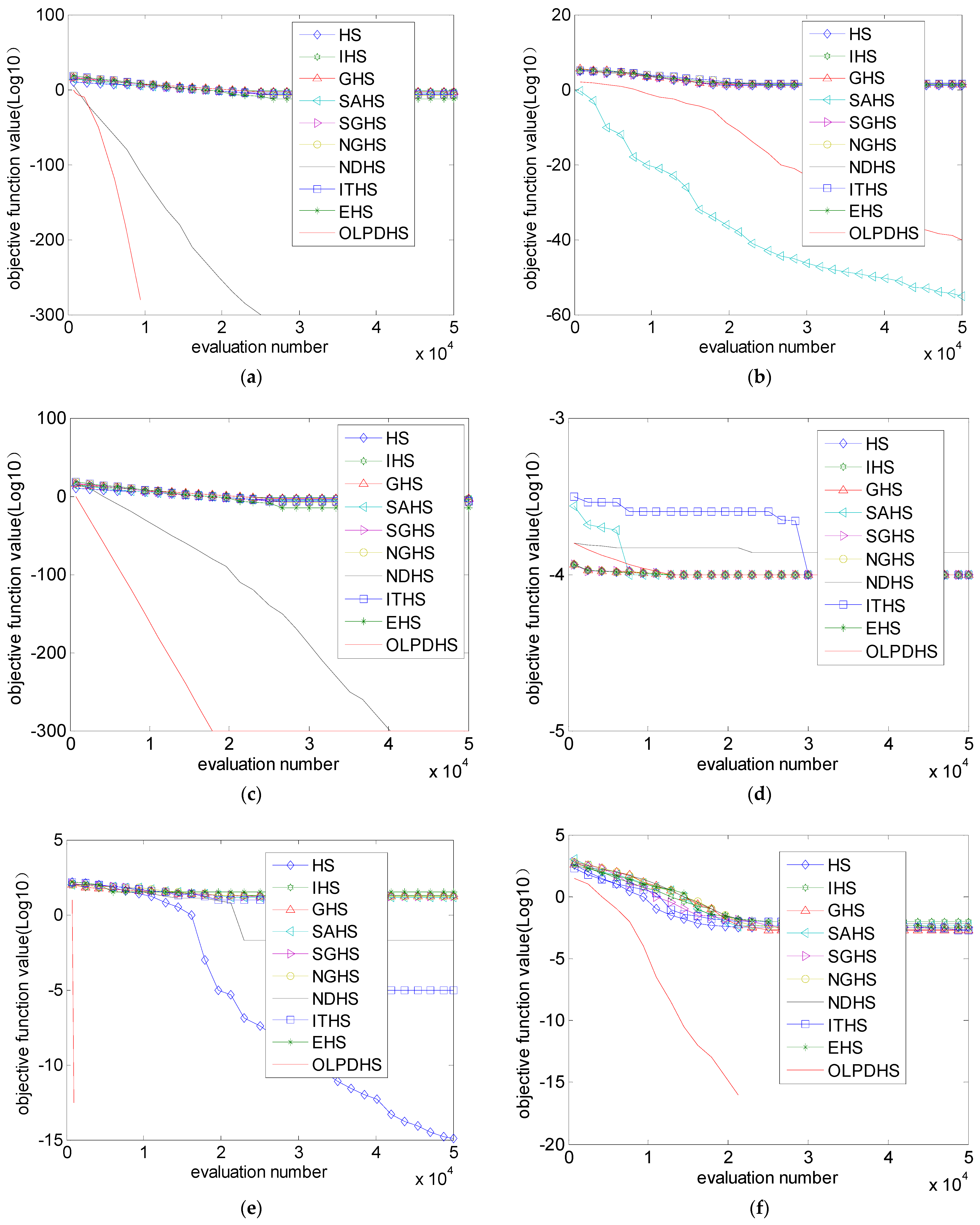
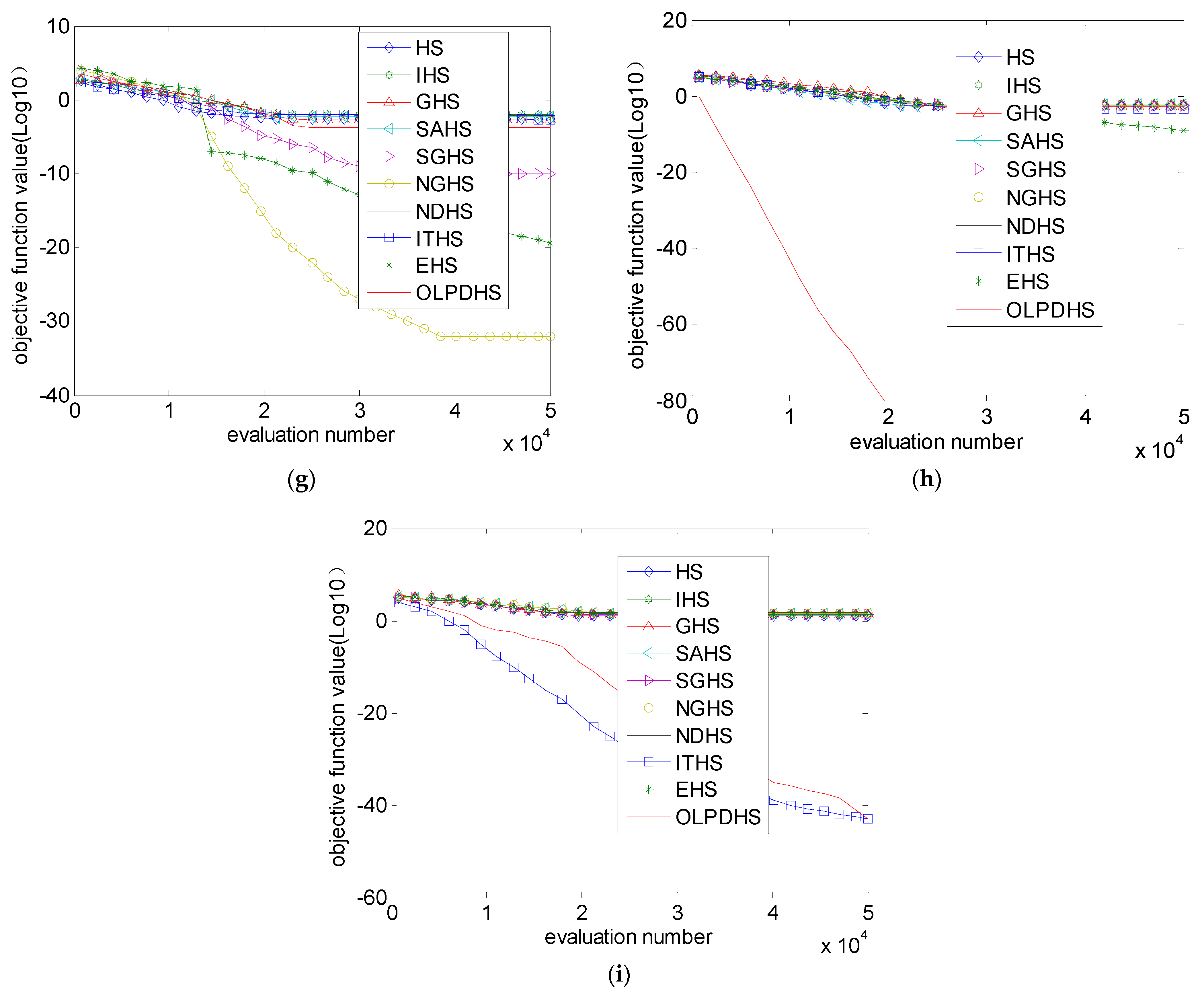
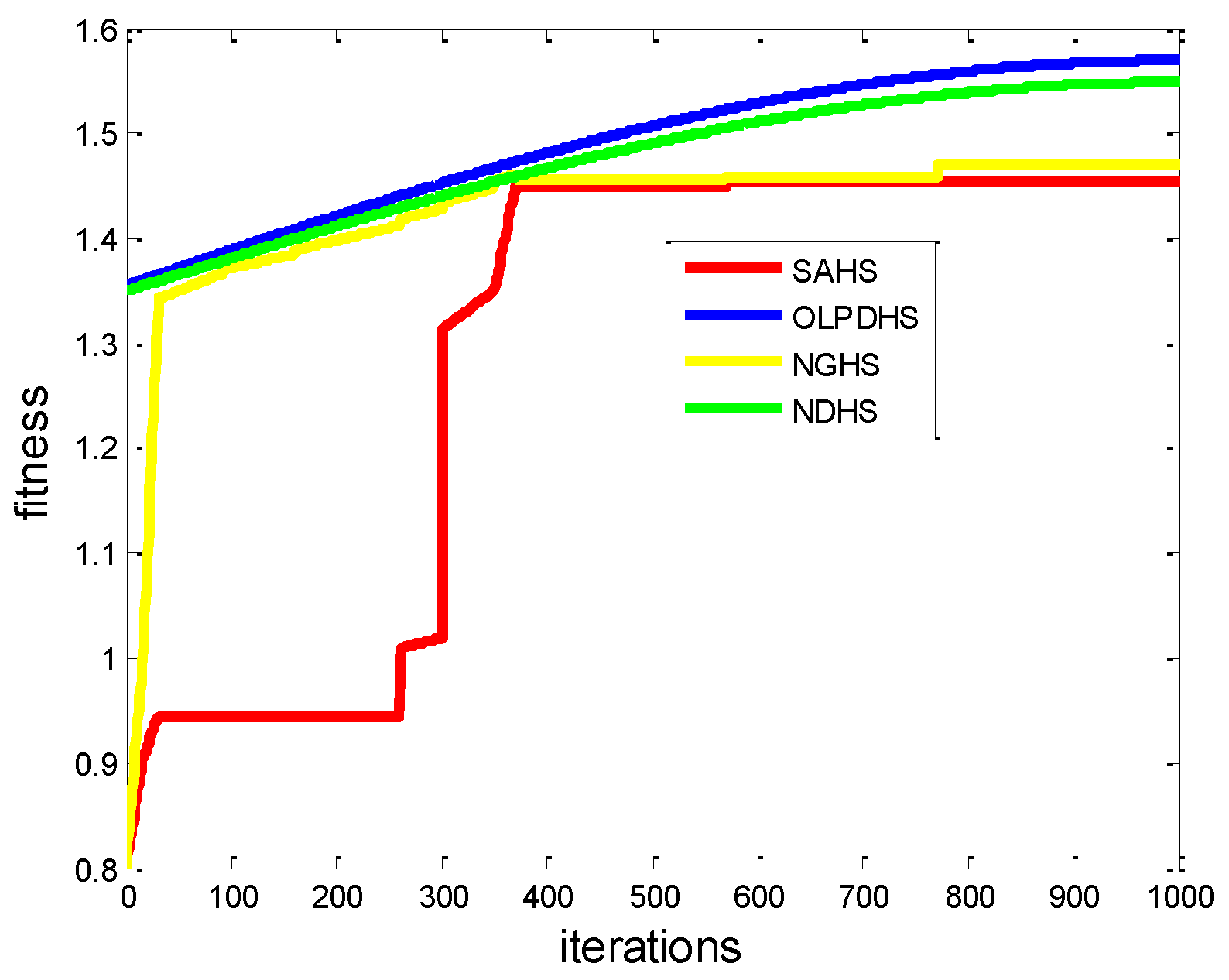
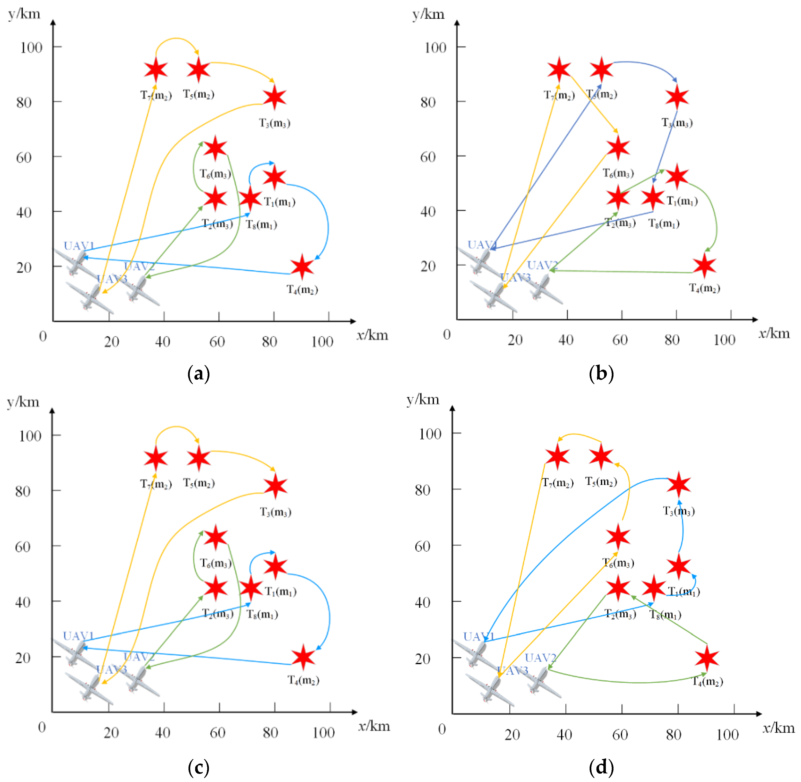
In this paper, the complex task set was decomposed into sub-tasks suitable for a single UAV, and then the task-allocation problem was described and defined from the aspects of task rewards and task cost. The UAV’s own constraints and mission constraints were defined. The mathematical model of task assignment was established, being more suitable for actual battlefield environment. The OLPDHS algorithm was proposed through discussion of exploration performance and convergence performance and its parameter values (HMCR > 0.9, PAR is in the interval [0.3, 0.7], HMS is appropriate in [5, 40]) were given via a number of simulation experiments. In comparison with IHS, GHS, SAHS, SGHS, NGHS, NDHS, EHS and ITHS, the superior performance of OLPDHS was proven by a number of simulation experiments. A multi-UAV cooperative task-allocation example was designed to verify the superior performance of OLPDHS (Fitness is 1.5491, time cost is 0.0819). This is the first application of HS to the multi-UAV cooperative task-allocation problem. These performance qualities are ideal for helping decision-makers devise allocation schemes.

In the environment or in the system itself at runtime, real-world scenarios abound with the aforementioned dynamism. It is necessary for cooperative systems to deal with this dynamism to keep the execution and results level. Future work must study the dynamic redistribution problem, which is closer to real-world scenarios, focusing on how to establish the redistribution problem model in a dynamic environment, so that decision makers can make effective decisions in the battlefield’s changeable environment.

References

1. Shirzadeh, M.; Asl, H.J.; Amirkhani, A.; Jalali, A.A. Vision-based control of a quadrotor utilizing artificial neural networks for tracking of moving targets. Eng. Appl. Artif. Intell. 2017, 58, 34–48. [Google Scholar] [CrossRef]
2. Sun, X.; Cai, C.; Yang, J.; Shen, X. Route evaluation for unmanned aerial vehicle based on type-2 fuzzy sets. Eng. Appl. Artif. Intell. 2015, 39, 132–145. [Google Scholar] [CrossRef]
3. Nonami, K.; Kendoul, F.; Suzuki, S.; Nonami, K.; Wang, W. Autonomous Flying Robots: Unmanned Aerial Vehicles and Micro Aerial Vehicles; Springer Science & Business Media: Berlin/Heidelberg, Germany, 2010. [Google Scholar]
4. Smith, K.; Stengel, R.F. Autonomous control of uninhabited combat air vehicles in heavily-trafficked military airspace. In Proceedings of the 14th AIAA Aviation Technology, Integration, and Operations Conference, Atlanta, GA, USA, 16–20 June 2014; p. 2287. [Google Scholar]
5. Qu, X.; Zhang, W.; Wang, X. Research of UAVs’ attack strategy under uncertain condition. Flight Dyn. 2015, 4, 021. [Google Scholar]
6. Song, B.D.; Kim, J.; Kim, J.; Park, H.; Morrison, J.R.; Shim, D.H. Persistent UAV service: An improved scheduling formulation and prototypes of system components. J. Intell. Robot. Syst. 2014, 74, 221–232. [Google Scholar] [CrossRef]
7. Dias, M.B.; Zlot, R.; Kalra, N.; Stentz, A. Market-based multirobot coordination: A survey and analysis. Proc. IEEE 2006, 94, 1257–1270. [Google Scholar] [CrossRef] [Green Version]
8. Johnson, L.B.; Choi, H.L.; How, J.P. The role of information assumptions in decentralized task allocation: A tutorial. IEEE Control Syst. Mag. 2016, 36, 45–58. [Google Scholar]
9. Kim, M.H.; Kim, S.P.; Lee, S. Social-welfare based task allocation for multi-robot systems with resource constraints. Comput. Ind. Eng. 2016, 63, 994–1002. [Google Scholar] [CrossRef]
10. Trigui, S.; Koubaa, A.; Cheikhrouhou, O.; Youssef, H.; Bennaceur, H.; Sriti, M.F.; Javed, Y. A distributed market-based algorithm for the multi-robot assignment problem. Procedia Comput. Sci. 2017, 32, 1108–1114. [Google Scholar] [CrossRef] [Green Version]
11. Yin, G.Y.; Zhou, S.L.; He, P.C.; Lei, X.J.; Kang, Y.H. Research status and development trend of cooperative task assignment of multiple UAVs abroad. Maneuverable Missile 2016, 5, 54–58. [Google Scholar] [CrossRef]
12. Zhu, Y.; Zhang, T.; Cheng, N. Research on cooperative mission planning of multiple UAVs. J. Syst. Simul. 2009, 20, 194–199. [Google Scholar]
13. Han, Q. Research on cooperate task allocation of multiple UAVs based on PSO algorithm. J. Ordnance Equip. Eng. 2019, 40, 74–78. [Google Scholar] [CrossRef]
14. Liu, Y. Research on Tasks Assignment and Tracks Planning of Multi-UAVs Cooperative Operation; Shenyang Aerospace University: Shenyang, China, 2019. [Google Scholar]
15. Korsah, G.A.; Stentz, A.; Dias, M.B. A comprehensive taxonomy for multi-robot task allocation. Int. J. Robot. Res. 2013, 32, 1495–1512. [Google Scholar] [CrossRef]
16. Rostami, A.S.; Mohanna, F.; Keshavarz, H.; Hosseinabadi, A.R. Solving multiple traveling salesman problem using the gravitational emulation local search algorithm. Appl. Math. Inf. Sci. 2015, 9, 1–11. [Google Scholar]
17. Omer, J.; Farges, J.L. Hybridization of nonlinear and mixed-integer linear programming for aircraft separation with trajectory recovery. IEEE Trans. Intell. Transp. Syst. 2013, 14, 1218–1230. [Google Scholar] [CrossRef]
18. Lincheng, S. Theory and Method of Autonomous Cooperative Control of Multiple UAVs; National Defense Industry Press: Beijing, China, 2013. [Google Scholar]
19. Nygard, K.E.; Chandler, P.R.; Pachter, M. Dynamic network flow optimization models for air vehicle resource allocation. In Proceedings of the 2001 American Control Conference, Arlington, VA, USA, 25–27 June 2001; IEEE: Piscataway, NJ, USA, 1963; Volume 3, pp. 1853–1858. [Google Scholar]
20. Edison, E.; Shima, T. Integrated task assignment and path optimization for cooperating uninhabited aerial vehicles using genetic algorithms. Comput. Oper. Res. 2011, 38, 340–356. [Google Scholar] [CrossRef]
21. Zorlu, O. Routing unmanned aerial vehicles as adapting to capacitated vehicle routing problem with genetic algorithms. In Proceedings of the International Conference on Recent Advances in Space Technologies, Istanbul, Turkey, 16–19 June 2015; IEEE: Piscataway, NJ, USA, 1963; pp. 675–679. [Google Scholar]
22. Mun, S.; Cho, Y.H. Modified harmony search optimization for constrained design problems. Expert Syst. Appl. 2012, 39, 419–423. [Google Scholar] [CrossRef]
23. Alatas, B. Chaotic harmony search algorithms. Appl. Math. Comput. 2010, 216, 2687–2699. [Google Scholar] [CrossRef]
24. Niu, W.J.; Feng, Z.K.; Jiang, Z.Q. Enhanced harmony search algorithm for sustainable ecological operation of cascade hydropower reservoirs in river ecosystem. Environ. Res. Lett. 2021, 16, 110–120. [Google Scholar] [CrossRef]
25. Mahalingam, S.K.; Nagarajan, L.; Salunkhe, S. Harmony search algorithm for minimizing assembly variation in non-linear Assembly. Appl. Sci. 2021, 11, 9213. [Google Scholar] [CrossRef]
26. Min, J.C. An analysis of children’s mental health based on HIS-FCM. Microcomput. Appl. 2020, 36, 62–64. [Google Scholar]
27. Shams, M.; El-Banbi, A.; Sayyouh, H. Harmony search optimization applied to reservoir engineering assisted history matching. Pet. Explor. Dev. 2020, 47, 148–154. [Google Scholar] [CrossRef]
28. Tao, Y.S.; Wang, K.X.; Yang, J. Hybridizing information gain and harmony search for feature selection on speech emotion. J. Chin. Comput. Syst. 2017, 38, 1164–1168. [Google Scholar]
29. Fu, S.; Wang, H.D. Indoor positioning of wireless network based on harmony search algorithm optimizing neural network. J. Nanjing Univ. Sci. Technol. 2017, 41, 428–433. [Google Scholar]
30. Das, S.; Mukhopadhyay, A.; Roy, A. Exploratory power of the harmony search algorithm: Analysis and improvements for global numerical optimization. IEEE Trans. Syst. Man Cybern. Part B Cybern. 2011, 41, 89–106. [Google Scholar] [CrossRef]
31. Huange, X.; Quli, M.; Tao, R. Mission assignment planning method for heterogeneous UAV cooperation based on sales contract strategy and PSO algorithm. J. Nav. Univ. Eng. 2018, 30, 1–5. [Google Scholar]
32. Zhang, T.; Yan, J.B. Numeric Analysis. Metalurgical; Industry Press: Beijing, China, 2007. [Google Scholar]
33. Tizhoosh, H.R. Opposition-based learning: A new scheme for machine intelligence. In Proceedings of the CIMCA/IAWTIC, Vienna, Austria, 28–30 November 2005; IEEE Computers Society: Piscataway, NJ, USA, 1963. [Google Scholar]
34. Wu, W.H.; Guo, X.F.; Zhou, S.Y. Self-adaptive differential algorithm with random neighborhood-based strategy and generalized opposition-based learning. Syst. Eng. Electron. 2021, 43, 1928–1942. [Google Scholar]
35. Rahnamayan, S.; Tizhoosh, H.R.; Salama, M. Opposition-based differential evolution. IEEE Trans. Evolut. Comput. 2018, 12, 6479. [Google Scholar]
36. Zhang, Y.; Yuan, S.J.; Da, L.X. Adaptive opposition-based learning cuckoo algorithm based on local search enhancement strategy. Math. Pract. Theory 2020, 50, 191–200. [Google Scholar]
37. Mahdavi, M.; Fesanghary, M.; Damangir, E. An improved harmony search algorithm for solving optimization problems. Appl. Math. Comput. 2007, 188, 1567–1579. [Google Scholar] [CrossRef]
38. Omran, M.G.H.; Mahdavi, M. Global-best harmony search. Appl. Math. Comput. 2008, 198, 643–656. [Google Scholar] [CrossRef]
39. Wang, C.M.; Huang, Y.F. Self-adaptive harmony search algorithm for optimization. Expert Syst. Appl. 2010, 37, 2826–2837. [Google Scholar] [CrossRef]
40. Pan, Q.K.; Suganthan, P.N.; Tasgetiren, M.F.; Liang, J.J. A self-adaptive global best harmony search algorithm for continuous optimization problems. Appl. Math. Comput. 2010, 216, 830–848. [Google Scholar] [CrossRef]
41. Zou, D.; Gao, L.; Wu, J.; Li, S. Novel global harmony search algorithm for unconstrained problems. Neurocomputing 2010, 73, 3308–3318. [Google Scholar] [CrossRef]
42. Chen, J.; Pan, Q.; Li, J. Harmony search algorithm with dynamic control parameters. Appl. Math. Comput. 2012, 219, 592–604. [Google Scholar] [CrossRef]
43. Yadav, P.; Kumar, R.; Panda, S.K.; Chang, C.S. An intelligent tuned harmony search algorithm for optimization. Inf. Sci. 2012, 196, 47–72. [Google Scholar] [CrossRef]
44. Scerri, P.; Farinelli, A.; Okamoto, S.; Tambe, M. Allocating tasks in extreme teams. In Proceedings of the 4th International Joint Conference on Autonomous Agents and Multiagent Systems, Utrecht, The Netherlands, 25–29 July 2005; ACM: New York, NY, USA, 1947; pp. 727–734. [Google Scholar]
45. Ferreira, P.R., Jr.; Boffo, F.S.; Bazzan, A.L. A swarm based approximated algorithm to the extended generalized assignment problem (e-gap). In Proceedings of the 6th International Joint Conference on Autonomous Agents And Multiagent Systems, AAMAS, Honolulu HI, USA, 14–18 May 2007; ACM: New York, NY, USA, 1947; pp. 1231–1233. [Google Scholar]
46. Ferreira, P.R., Jr.; Dos Santos, F.; Bazzan, A.L.; Epstein, D.; Waskow, S.J. RoboCup Rescue as multiagent task allocation among teams: Experiments with task interdependencies. Auton. Agents Multi-Agent Syst. 2010, 20, 421–443. [Google Scholar] [CrossRef]
47. Ikemoto, Y.; Miura, T.; Asama, H. Adaptive division of labor control for robot group. In Proceedings of the International Conference on Intelligent Robot and Systems, St. Louis, MO, USA, 11–15 October 2009; pp. 2409–2414. [Google Scholar]
48. Schwarzrock, J.; Zacarias, I.; Bazzan, A.L.C.; de Araujo Fernandes, R.Q.; Moreira, L.H.; de Freitas, E.P. Solving task allocation problem in multi unmanned aerial vehicles systems using swarm intelligence. Eng. Appl. Artif. Intell. 2018, 72, 10–20. [Google Scholar] [CrossRef]
49. Amorim, J.C.; Alves, V.; de Freitas, E.P. Assessing a swarm-GAP based solution for the task allocation problem in dynamic scenarios. Expert Syst. Appl. 2020, 152, 113437. [Google Scholar] [CrossRef]
50. Landén, D.; Heintz, F.; Doherty, P. Complex task allocation in mixed-initiative delegation: A UAV case study. In Proceedings of the International Conference on Principles and Practice of Multi-Agent Systems, Kolkata, India, 12–15 November 2010; Springer: Berlin/Heidelberg, Germany, 2012; pp. 288–303. [Google Scholar]
51. Ibri, S.; Nourelfath, M.; Drias, H. A multi-agent approach for integrated emergency vehicle dispatching and covering problem. Eng. Appl. Artif. Intell. 2012, 5, 554–565. [Google Scholar] [CrossRef]
52. Tolmidis, A.T.; Petrou, L. Multi-objective optimization for dynamic task allocation in a multi-robot system. Eng. Appl. Artif. Intell. 2013, 26, 1458–1468. [Google Scholar] [CrossRef]
53. Shima, T.; Rasmussen, S.J.; Sparks, A.G.; Passino, K.M. Multiple task assignments for cooperating uninhabited aerial vehicles using genetic algorithms. Comput. Oper. Res. 2006, 33, 3252–3269. [Google Scholar] [CrossRef]
54. Fei, S.; Yan, C.; Lin, S. Collaborative multi-task assignment of unmanned aerial vehicles based on ant colony algorithm. Chin. J. Aeronaut. 2008, 1, 189–196. [Google Scholar]
55. Wen, G. Research and Application of Target Assignment Problem Based on Evolutionary Hungarian Algorithm; Xidian University: Xi’an, China, 2013. [Google Scholar]
56. Jin, Z.; Hao, G.; Tong, C. Weapon-target assignment based on adaptable hungarian algorithm. Acta Armamentarh 2021, 42, 1339–1344. [Google Scholar]
57. Bellingham, J.; Tillerson, M.; Richards, A.; How, J.P. Multi-task allocation and path planning for cooperating UAVs. In Cooperative Control: Models, Applications and Algorithms; Springer: Boston, MA, USA, 2003; pp. 23–41. [Google Scholar]
Figure 1. Mapping relationship between particle coding and UAV task assignment problem.
Electronics 11 01171 g001
Figure 2. The expected population variance of OLPDHS with HMCR value for Sphere and Rastrigin: (a) Sphere: [−50, 100]; (b) Sphere: [−100, 50]; (c) Rastrigin: [−50, 100]; (d) Rastrigin: [−100, 50].
Electronics 11 01171 g002
Figure 3. Convergence of OLPDHS with different HMCR values for Sphere and Rastrigin: (a) Sphere: [−50, 100]; (b) Sphere: [−100, 50]; (c) Rastrigin: [−50, 100]; (d) Rastrigin: [−100, 50].
Electronics 11 01171 g003
Figure 4. The optimization curve for different values of the parameter PAR: (a) f 1 ; (b) f 2 ; (c) f 3 ; (d) f 4 ; (e) f 5 ; (f) f 6 ; (g) f 7 ; (h) f 8 ; (i) f 9 .
Electronics 11 01171 g004aElectronics 11 01171 g004b
Figure 5. The optimization curve for different values of the parameter HMS: (a) f 1 ; (b) f 2 ; (c) f 3 ; (d) f 4 ; (e) f 5 ; (f) f 6 ; (g) f 7 ; (h) f 8 ; (i) f 9 .
Electronics 11 01171 g005aElectronics 11 01171 g005b
Figure 6. The evolution of optimum objective function value with 10 algorithms for 9 functions: (a) f 1 ; (b) f 2 ; (c) f 3 ; (d) f 4 ; (e) f 5 ; (f) f 6 ; (g) f 7 ; (h) f 8 ; (i) f 9 .
Electronics 11 01171 g006aElectronics 11 01171 g006b
Figure 7. The battlefield environment diagram.
Electronics 11 01171 g007
Figure 8. The convergence curves of fitness of two algorithms.
Electronics 11 01171 g008
Figure 9. The average times of the four algorithms running independently 10 times.
Electronics 11 01171 g009
Figure 10. The schematic diagram of task assignment results of two algorithms: (a) OLPDHS; (b) SAHS; (c) NDHS; (d) NGHS.
Electronics 11 01171 g010