
Hybrid Feature Reduction Using PCC-Stacked Autoencoders for Gold/Oil Prices Forecasting under COVID-19 Pandemic

 ,
,  , , and
Abstract
:1. Introduction
2. Literature Review
- Analysis of recently published COVID-19 data sets along with the crude oil, and gold prices during that global health crisis and studying the impact of high spread and mortality rates, precautionary measures, and vaccinations on the prices of such commodities.
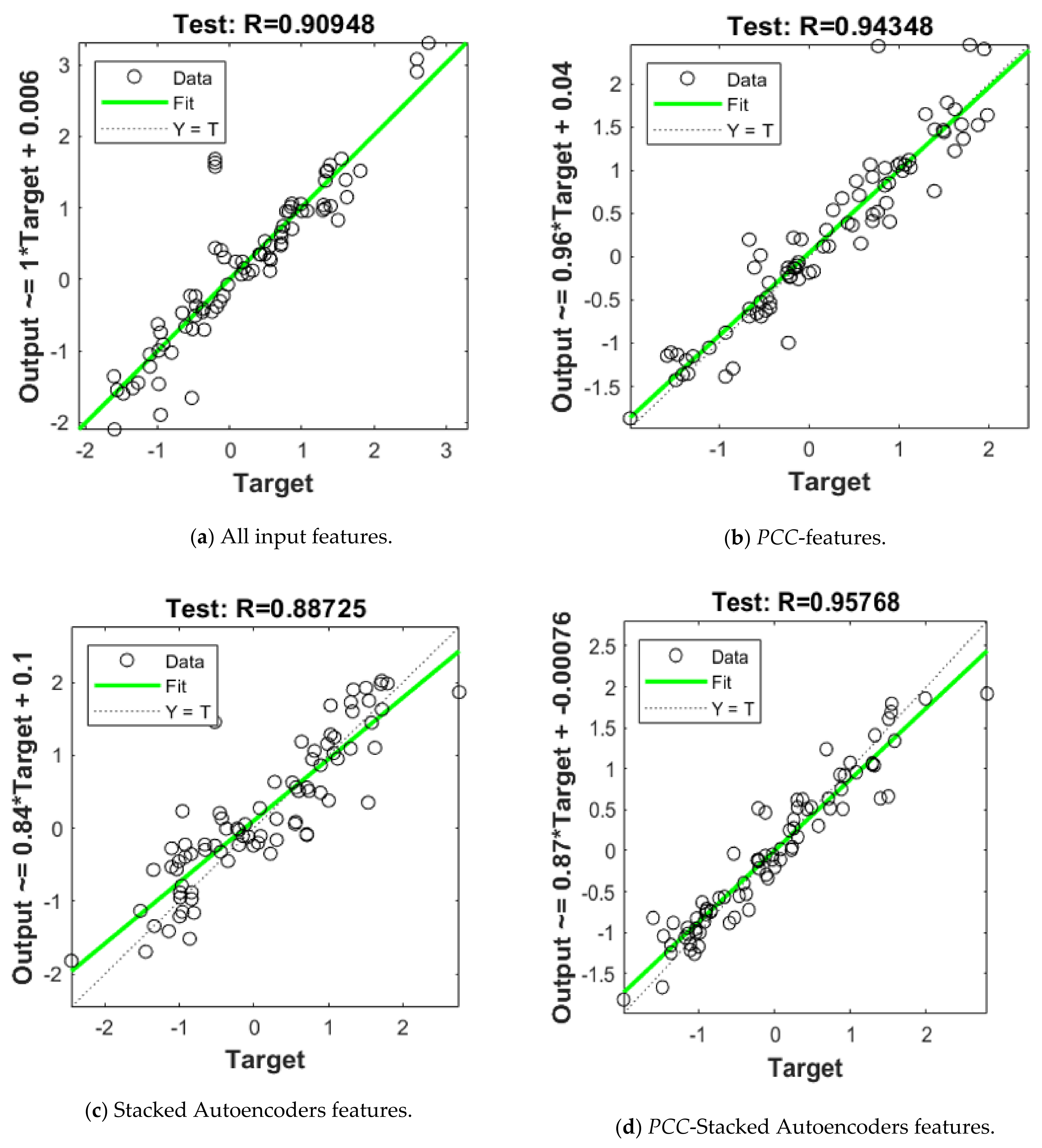
- Deep Autoencoders are integrated with the correlation analysis approach in selecting the key features that affect the accuracy of the forecasting models.
- The Bayesian regularization-backpropagation algorithm is utilized to avoid the overfitting of data which is a major drawback of training ANNs on the small-size datasets.
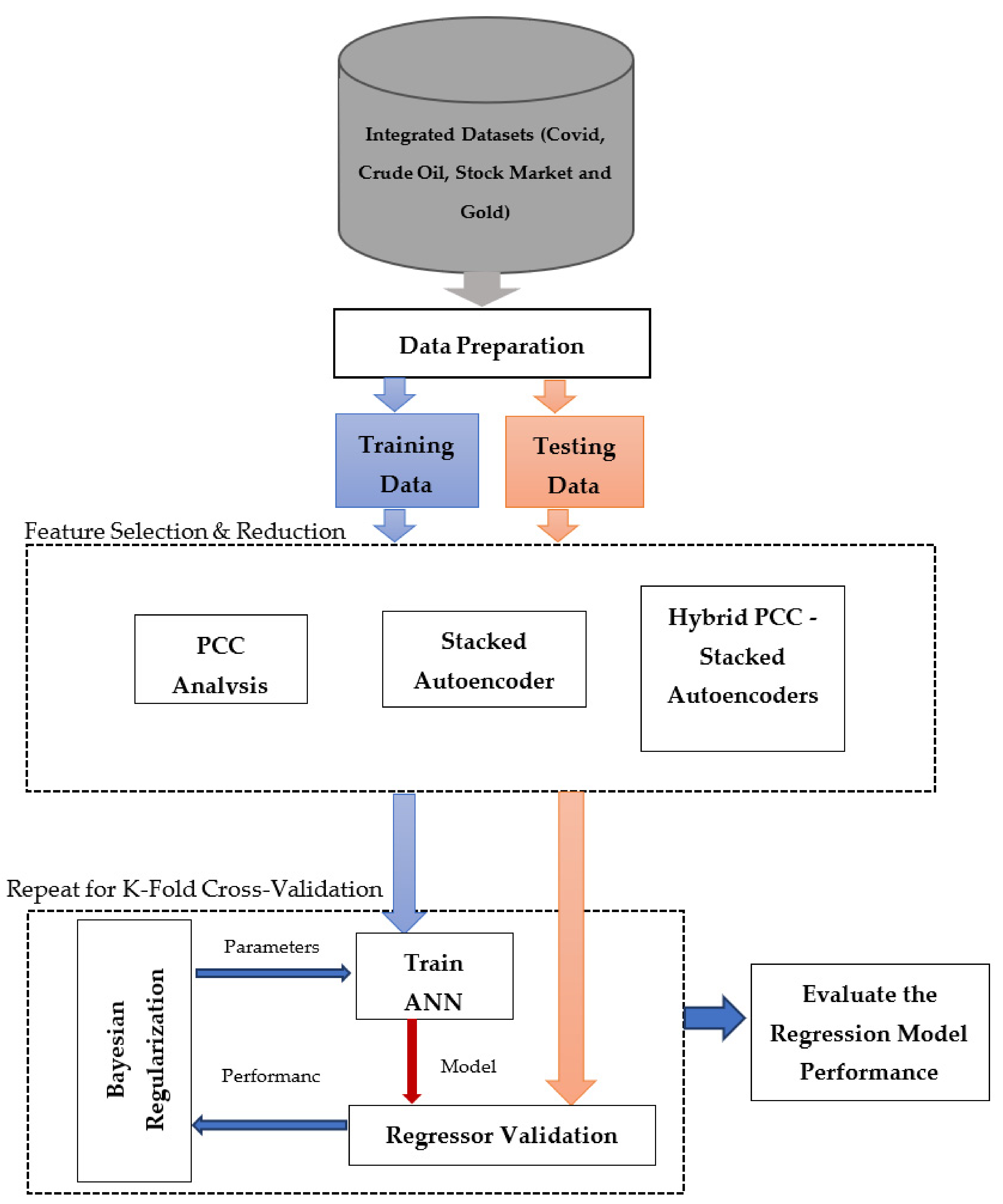
3. Methods
3.1. Data Exploration and Hypothesis Testing
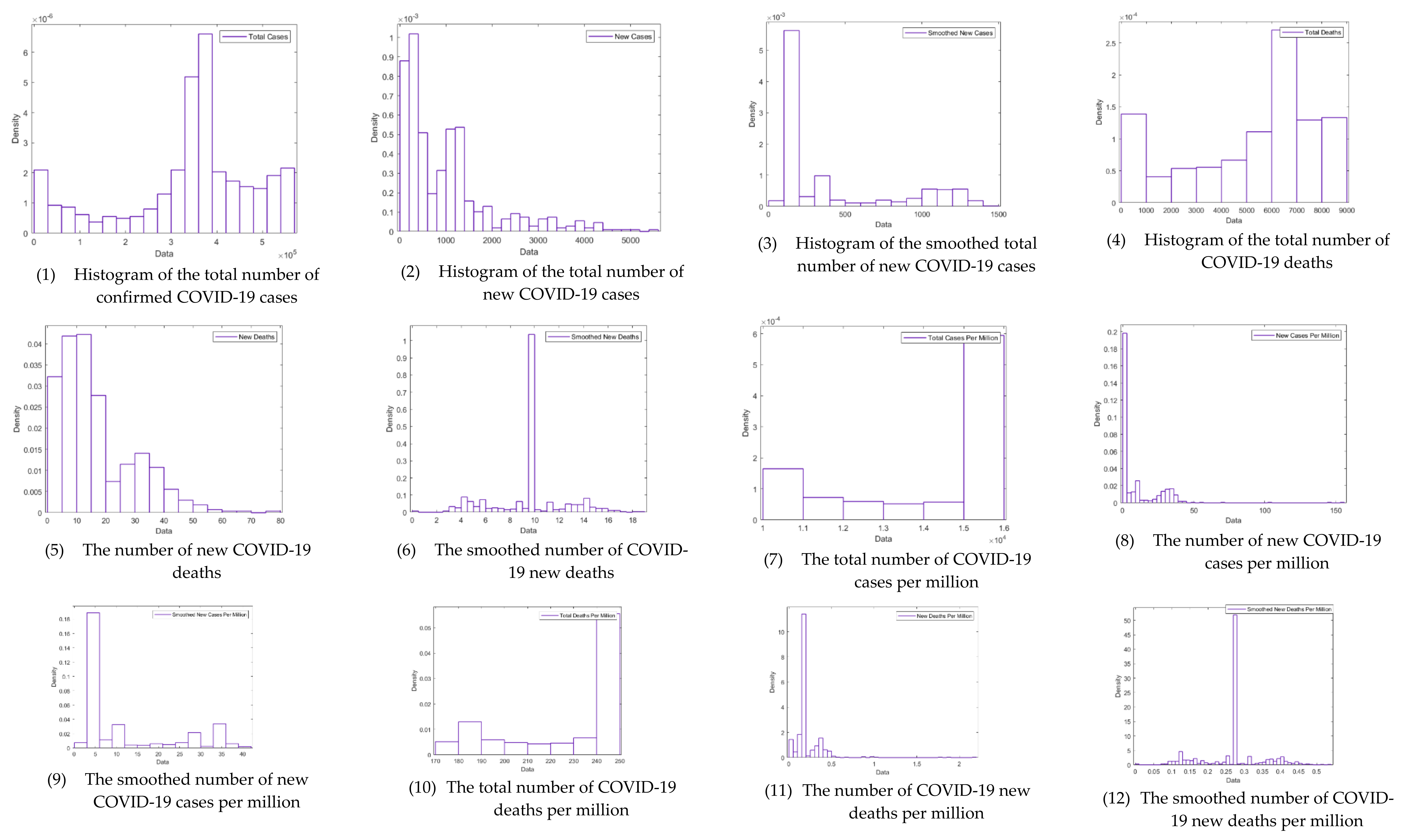
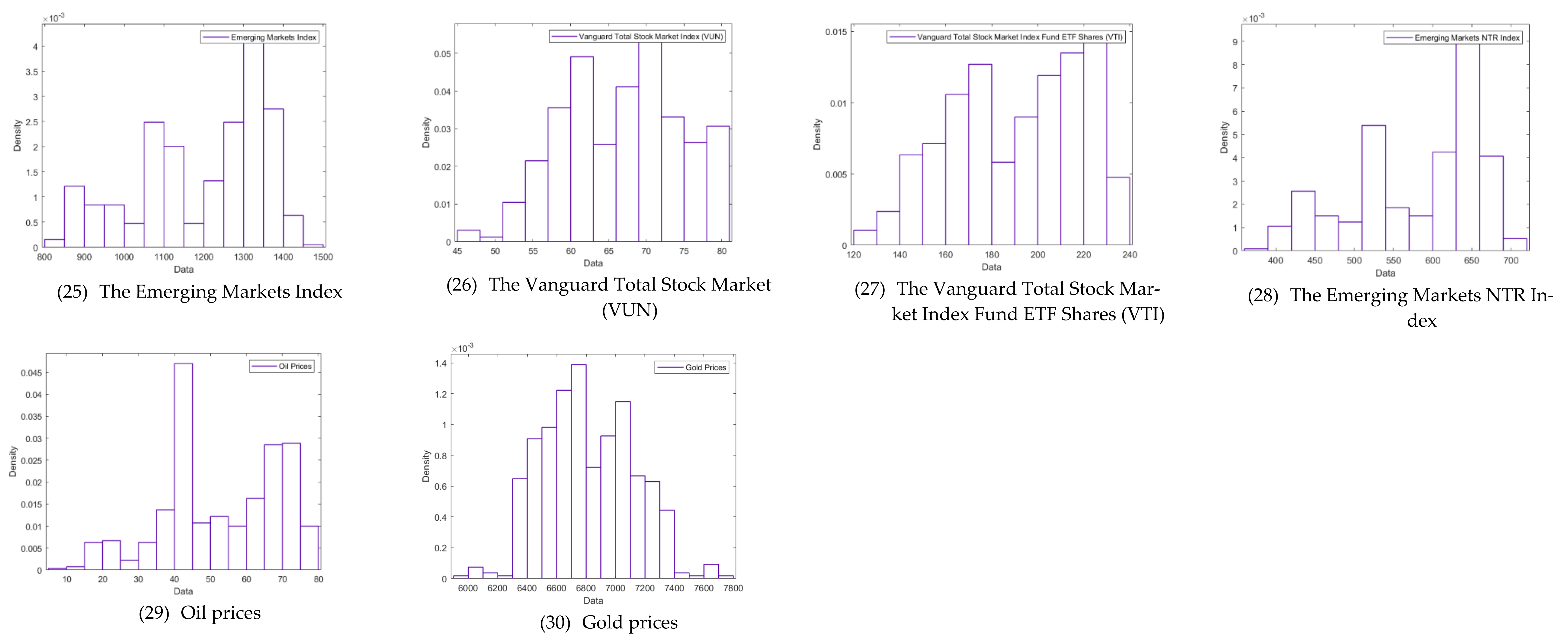
3.1.1. Data Exploration and Preprocessing
3.1.2. Hypothesis Testing
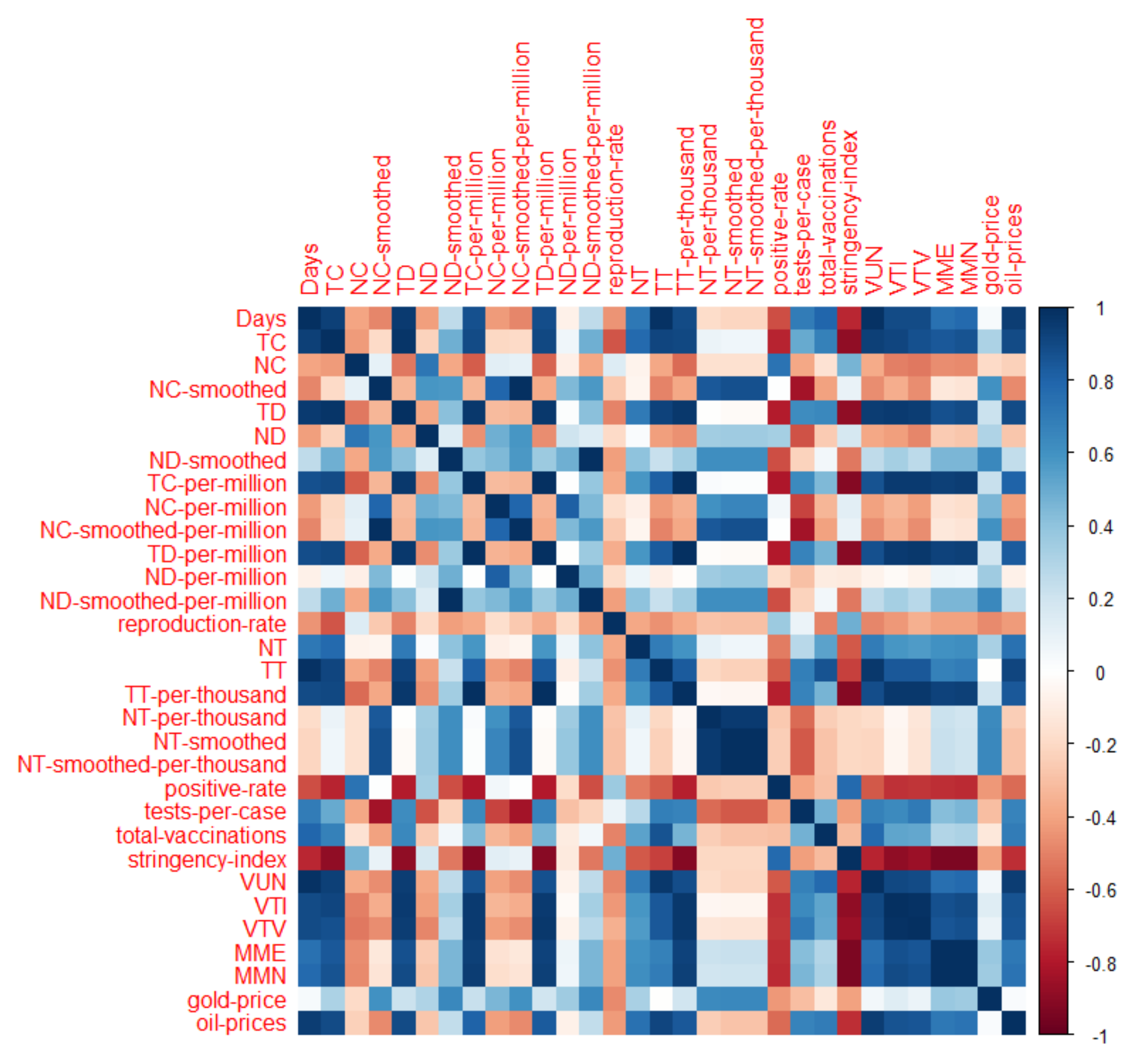
3.2. Pearson Correlation Coefficient Analysis
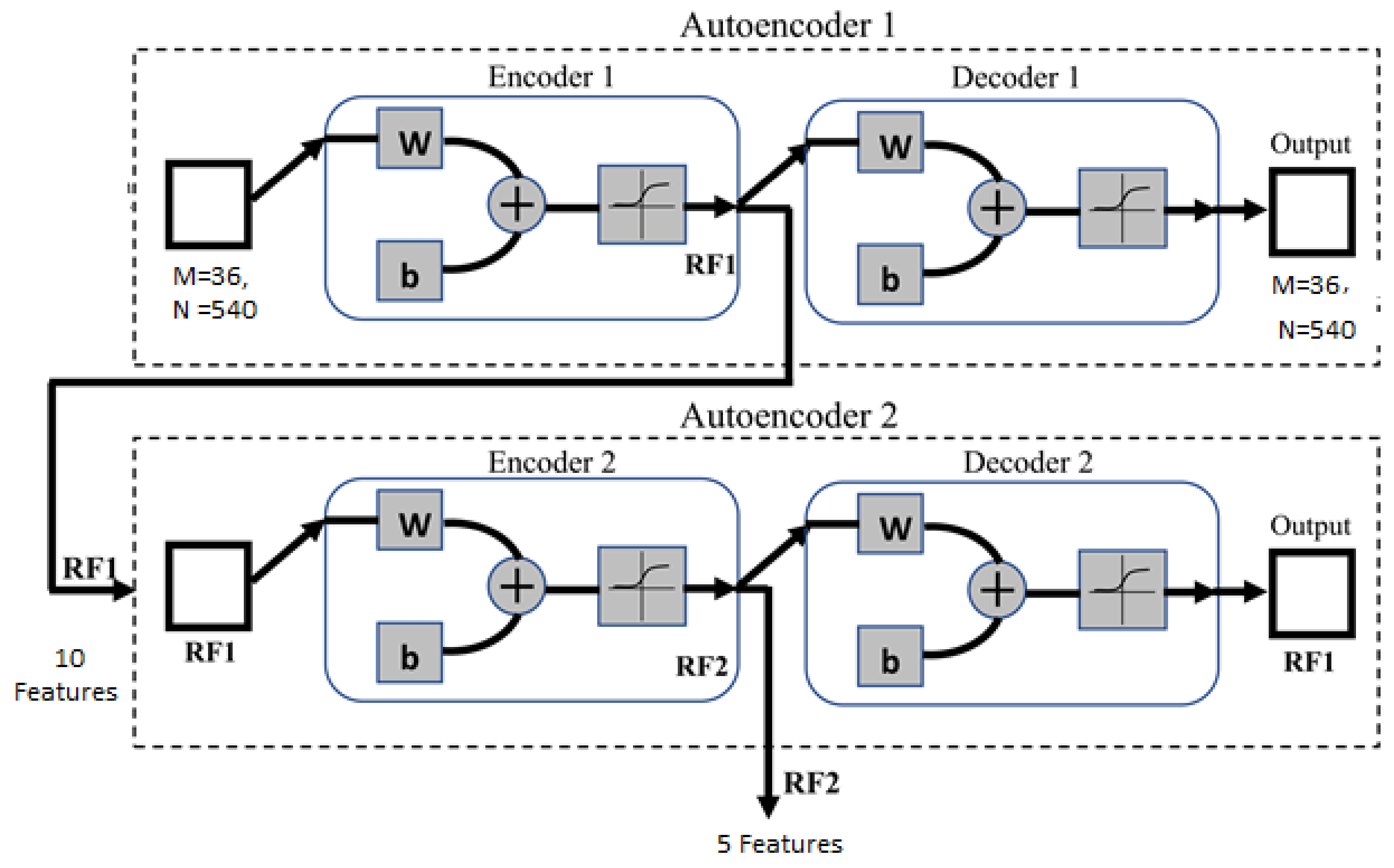
3.3. Stacked Deep Autoencoder
3.4. Bayesian Optimization for Regularization of NN Regressor
- Initialize the weights, , and the regularization parameters , .
- Apply the Levenberg–Marquardt algorithm to minimize , the objective function.
- Compute and which are the effective, and a total number of parameters in the network , where and is the Jacobian matrix of the training errors.
- Compute new estimation for the regularization parameters , and .
- Repeat steps 2 to 4 until attaining convergence.
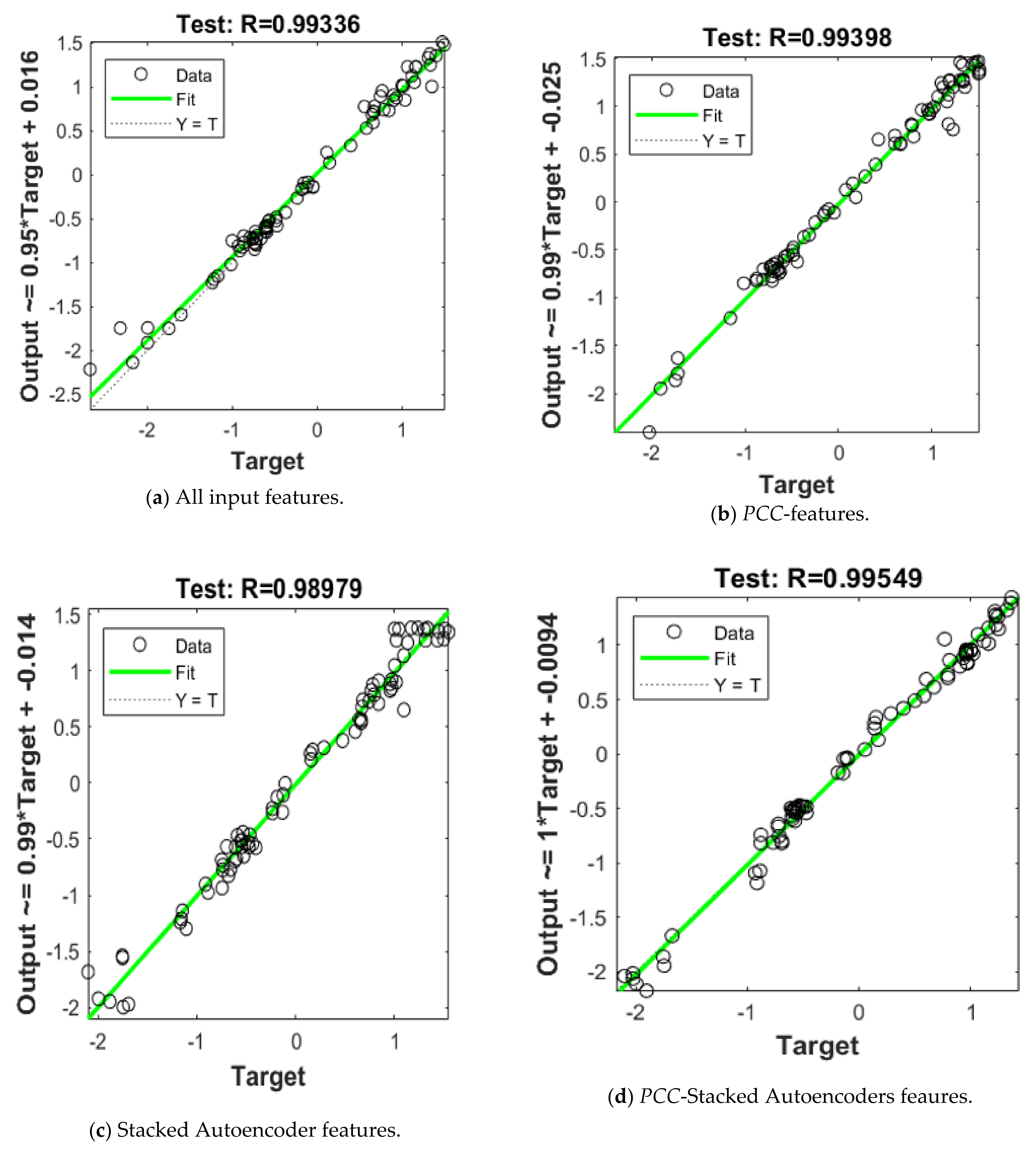
4. Results and Discussion
5. Conclusions
Author Contributions
Funding
Acknowledgments
Conflicts of Interest
References
- Singleton, K.J. Investor Flows and the 2008 Boom/Bust in Oil Prices. Manag. Sci. 2014, 60, 300–318. [Google Scholar] [CrossRef] [Green Version]
- Bernanke, B.S. Irreversibility, Uncertainty, and Cyclical Investment. Q. J. Econ. 1983, 98, 85. [Google Scholar] [CrossRef]
- Soytas, U.; Sari, R.; Hammoudeh, S.; Hacihasanoglu, E. World Oil Prices, Precious Metal Prices and Macroeconomy in Turkey. Energy Policy 2009, 37, 5557–5566. [Google Scholar] [CrossRef]
- Baur, D.G.; Lucey, B.M. Is Gold a Hedge or a Safe Haven? An Analysis of Stocks, Bonds and Gold. Financ. Rev. 2010, 45, 217–229. [Google Scholar] [CrossRef]
- Mensi, W.; Reboredo, J.C.; Ugolini, A. Price-Switching Spillovers between Gold, Oil, and Stock Markets: Evidence from the USA and China during the COVID-19 Pandemic. Resour. Policy 2021, 73, 102217. [Google Scholar] [CrossRef]
- Nicola, M.; Alsafi, Z.; Sohrabi, C.; Kerwan, A.; Al-Jabir, A.; Iosifidis, C.; Agha, M.; Agha, R. The Socio-Economic Implications of the Coronavirus Pandemic (COVID-19): A Review. Int. J. Surg. 2020, 78, 185–193. [Google Scholar] [CrossRef]
- Bakas, D.; Triantafyllou, A. Commodity Price Volatility and the Economic Uncertainty of Pandemics. Econ. Lett. 2020, 193, 109283. [Google Scholar] [CrossRef]
- Sharif, A.; Aloui, C.; Yarovaya, L. COVID-19 Pandemic, Oil Prices, Stock Market, Geopolitical Risk and Policy Uncertainty Nexus in the US Economy: Fresh Evidence from the Wavelet-Based Approach. Int. Rev. Financ. Anal. 2020, 70, 101496. [Google Scholar] [CrossRef]
- Yan, L.; Zhu, Y.; Wang, H. Selection of Machine Learning Models for Oil Price Forecasting: Based on the Dual Attributes of Oil. Discret. Dyn. Nat. Soc. 2021, 2021, 1–16. [Google Scholar] [CrossRef]
- Arfaoui, M.; ben Rejeb, A. Oil, Gold, US Dollar and Stock Market Interdependencies: A Global Analytical Insight. Eur. J. Manag. Bus. Econ. 2017, 26, 278–293. [Google Scholar] [CrossRef]
- Zhang, Y.; Hamori, S. Forecasting Crude Oil Market Crashes Using Machine Learning Technologies. Energies 2020, 13, 2440. [Google Scholar] [CrossRef]
- Moshiri, S.; Foroutan, F. Forecasting Nonlinear Crude Oil Futures Prices. Energy J. 2006, 27, 81–95. [Google Scholar] [CrossRef]
- Zhang, J.L.; Zhang, Y.J.; Zhang, L. A Novel Hybrid Method for Crude Oil Price Forecasting. Energy Econ. 2015, 49, 649–659. [Google Scholar] [CrossRef]
- Kristjanpoller, R.W.; Hernández, P.E. Volatility of Main Metals Forecasted by a Hybrid ANN-GARCH Model with Regressors. Expert Syst. Appl. 2017, 84, 290–300. [Google Scholar] [CrossRef]
- Abdullah, S.N.; Zeng, X. Machine Learning Approach for Crude Oil Price Prediction with Artificial Neural Networks-Quantitative (ANN-Q) Model. In Proceedings of the International Joint Conference on Neural Networks, Barcelona, Spain, 18–23 July 2010. [Google Scholar] [CrossRef] [Green Version]
- Wu, Y.X.; Wu, Q.B.; Zhu, J.Q. Improved EEMD-Based Crude Oil Price Forecasting Using LSTM Networks. Phys. Stat. Mech. Appl. 2019, 516, 114–124. [Google Scholar] [CrossRef]
- Cen, Z.; Wang, J. Crude Oil Price Prediction Model with Long Short Term Memory Deep Learning Based on Prior Knowledge Data Transfer. Energy 2019, 169, 160–171. [Google Scholar] [CrossRef]
- Kim, H.Y.; Won, C.H. Forecasting the Volatility of Stock Price Index: A Hybrid Model Integrating LSTM with Multiple GARCH-Type Models. Expert Syst. Appl. 2018, 103, 25–37. [Google Scholar] [CrossRef]
- Rapach, D.E.; Zhou, G. Time-series and Cross-sectional Stock Return Forecasting: New Machine Learning Methods. In Machine Learning for Asset Management; Wiley: Hoboken, NJ, USA, 2020; pp. 1–33. [Google Scholar]
- Wang, J.; Zhou, H.; Hong, T.; Li, X.; Wang, S. A Multi-Granularity Heterogeneous Combination Approach to Crude Oil Price Forecasting. Energy Econ. 2020, 91, 104790. [Google Scholar] [CrossRef]
- Chen, Y.; He, K.; Tso, G.K.F. Forecasting Crude Oil Prices: A Deep Learning Based Model. Procedia Comput. Sci. 2017, 122, 300–307. [Google Scholar] [CrossRef]
- Bashiri Behmiri, N.; Pires Manso, J.R. Crude Oil Price Forecasting Techniques: A Comprehensive Review of Literature. SSRN Electron. J. 2013, 1–32. [Google Scholar] [CrossRef]
- Sariev, E.; Germano, G. Bayesian Regularized Artificial Neural Networks for the Estimation of the Probability of Default. Quant. Financ. 2020, 20, 311–328. [Google Scholar] [CrossRef]
- Osman, H.; Ghafari, M.; Nierstrasz, O. The Impact of Feature Selection on Predicting the Number of Bugs. arXiv 2018, arXiv:1807.04486. [Google Scholar]
- Javed, F.; Thomas, I.; Memedi, M. A Comparison of Feature Selection Methods When Using Motion Sensors Data: A Case Study in Parkinson’s Disease. In Proceedings of the Annual International Conference of the IEEE Engineering in Medicine and Biology Society, Honolulu, HI, USA, 18–21 July 2018; Volume 2018, pp. 5426–5429. [Google Scholar] [CrossRef]
- Atteia, G.; Abdel Samee, N.; Zohair Hassan, H. DFTSA-Net: Deep Feature Transfer-Based Stacked Autoencoder Network for DME Diagnosis. Entropy 2021, 23, 1251. [Google Scholar] [CrossRef] [PubMed]
- Shamshirband, S.; Mosavi, A.; Rabczuk, T.; Nabipour, N.; Chau, K. Prediction of Significant Wave Height; Comparison between Nested Grid Numerical Model, and Machine Learning Models of Artificial Neural Networks, Extreme Learning and Support Vector Machines. Eng. Appl. Comput. Fluid Mech. 2020, 14, 805–817. [Google Scholar] [CrossRef]
- Samuelson, P.A. Proof That Properly Discounted Present Values of Assets Vibrate Randomly. Bell J. Econ. Manag. Sci. 1973, 4, 369. [Google Scholar] [CrossRef]
- Atteia, G.E.; Mengash, H.A.; Samee, N.A. Evaluation of Using Parametric and Non-Parametric Machine Learning Algorithms for COVID-19 Forecasting. Int. J. Adv. Comput. Sci. Appl. 2021, 12, 647–657. [Google Scholar] [CrossRef]
- Smalheiser, N.R. Data Literacy: How to Make Your Experiments Robust and Reproducible. In Data Literacy: How to Make Your Experiments Robust and Reproducible; Academic Press: Cambridge, MA, USA, 2017; pp. 1–282. [Google Scholar] [CrossRef]
- Arai, K. Combined Non-Parametric and Parametric Classification Method Depending on Normality of PDF of Training Samples. Int. J. Adv. Comput. Sci. Appl. 2021, 12, 310–316. [Google Scholar] [CrossRef]
- Chin, R.; Lee, B.Y. Principles and Practice of Clinical Trial Medicine; Elsevier: Amsterdam, The Netherlands, 2008. [Google Scholar] [CrossRef]
- Oh, J.; Suh, K.D. Real-Time Forecasting of Wave Heights Using EOF—Wavelet—Neural Network Hybrid Model. Ocean Eng. 2018, 150, 48–59. [Google Scholar] [CrossRef]
- Li, Y.; Bao, T.; Chen, Z.; Gao, Z.; Shu, X.; Zhang, K. A Missing Sensor Measurement Data Reconstruction Framework Powered by Multi-Task Gaussian Process Regression for Dam Structural Health Monitoring Systems. Measurement 2021, 186, 110085. [Google Scholar] [CrossRef]
- Hu, J.; Wang, J.; Ma, K. A Hybrid Technique for Short-Term Wind Speed Prediction. Energy 2015, 81, 563–574. [Google Scholar] [CrossRef]
- Yu, L.; Zhang, X.; Wang, S. Assessing Potentiality of Support Vector Machine Method in Crude Oil Price Forecasting. Eurasia J. Math. Sci. Technol. Educ. 2017, 13, 7893–7904. [Google Scholar] [CrossRef]
- Zhao, C.L.; Wang, B. Forecasting Crude Oil Price with an Autoregressive Integrated Moving Average (ARIMA) Model. Adv. Intell. Syst. Comput. 2014, 211, 275–286. [Google Scholar] [CrossRef]
- SenGupta, I.; Nganje, W.; Hanson, E. Refinements of Barndorff-Nielsen and Shephard Model: An Analysis of Crude Oil Price with Machine Learning. Ann. Data Sci. 2021, 8, 39–55. [Google Scholar] [CrossRef] [Green Version]
- Gers, F.A.; Schmidhuber, J.; Cummins, F. Learning to Forget: Continual Prediction with LSTM. Neural Comput. 2000, 12, 2451–2471. [Google Scholar] [CrossRef]
- Johns Hopkins University Center for Systems Science and Engineering at JHU. Available online: https://coronavirus.jhu.edu/ (accessed on 10 February 2022).
- World Daily Spot Prices for Crude Oil WTI and Brent—KAPSARC Data Portal. Available online: https://datasource.kapsarc.org (accessed on 16 January 2022).
- Gold Price Historical Data|Gold Price History|World Gold Council. Available online: https://www.gold.org/goldhub/data/gold-prices (accessed on 16 January 2022).
- Yahoo Finance—Stock Market Live, Quotes, Business & Finance News. Available online: https://finance.yahoo.com/ (accessed on 14 March 2022).
- Boslaugh, S. The Pearson Correlation Coefficient. In Statistics in a Nutshell, 2nd ed.; O’Reilly Media Inc.: Sebastopol, CA, USA, 2012; pp. 80–92. ISBN 9781449316822. [Google Scholar]
- Olshausen, B.A.; Field, D.J. Sparse Coding with an Overcomplete Basis Set: A Strategy Employed by V1? Vis. Res. 1997, 37, 3311–3325. [Google Scholar] [CrossRef] [Green Version]
- Smirnov, E.A.; Timoshenko, D.M.; Andrianov, S.N. Comparison of Regularization Methods for ImageNet Classification with Deep Convolutional Neural Networks. AASRI Procedia 2014, 6, 89–94. [Google Scholar] [CrossRef]
- Atri, H.; Kouki, S.; Gallali, M. imen The Impact of COVID-19 News, Panic and Media Coverage on the Oil and Gold Prices: An ARDL Approach. Resour. Policy 2021, 72, 102061. [Google Scholar] [CrossRef]
- He, X.J. Crude Oil Prices Forecasting: Time Series vs. SVR Models. J. Int. Technol. Inf. Manag. 2018, 27, 25–42. [Google Scholar]
- Weng, F.; Chen, Y.; Wang, Z.; Hou, M.; Luo, J.; Tian, Z. Gold Price Forecasting Research Based on an Improved Online Extreme Learning Machine Algorithm. J. Ambient. Intell. Humaniz. Comput. 2020, 11, 4101–4111. [Google Scholar] [CrossRef]
- He, K.; Chen, Y.; Tso, G.K.F. Price Forecasting in the Precious Metal Market: A Multivariate EMD Denoising Approach. Resour. Policy 2017, 54, 9–24. [Google Scholar] [CrossRef]
- Mohtasham Khani, M.; Vahidnia, S.; Abbasi, A. A Deep Learning-Based Method for Forecasting Gold Price with Respect to Pandemics. SN Comput. Sci. 2021, 2, 335. [Google Scholar] [CrossRef] [PubMed]
- Jabeur, S.B.; Mefteh-Wali, S.; Viviani, J.L. Forecasting Gold Price with the XGBoost Algorithm and SHAP Interaction Values. Ann. Oper. Res. 2021, 937, 1–21. [Google Scholar] [CrossRef]


| Variable | N | Mean | Std. Dev. | Min | Pctl. 25 | Pctl. 75 | Max |
|---|---|---|---|---|---|---|---|
| Days | 540 | 270.5 | 156.029 | 1 | 135.75 | 405.25 | 540 |
| TC | 540 | 337,834.8 | 146,380.1 | 1720 | 295,556.3 | 427,619.8 | 546,735 |
| NC | 540 | 1009.578 | 1020.568 | 0 | 314.75 | 1287.5 | 5439 |
| NC-smoothed | 540 | 407.053 | 412.462 | 0 | 129.429 | 672.286 | 1403.857 |
| TD | 540 | 5189.746 | 2653.295 | 16 | 3329.25 | 7088.25 | 8679 |
| ND | 540 | 16.054 | 13.059 | 0 | 6 | 24 | 77 |
| ND-smoothed | 540 | 9.581 | 2.993 | 0 | 8.964 | 9.857 | 18.857 |
| TC-per-million | 540 | 14,022.01 | 1969.446 | 10,260.16 | 12201.24 | 15,470.42 | 15,470.42 |
| NC-per-million | 540 | 10.427 | 16.008 | 0 | 1.528 | 13.78 | 153.902 |
| NC-smoothed-per-million | 540 | 11.518 | 11.671 | 0 | 3.662 | 19.023 | 39.724 |
| TD-per-million | 540 | 226.089 | 25.436 | 175.831 | 201.779 | 245.581 | 245.581 |
| ND-per-million | 540 | 0.23 | 0.182 | 0 | 0.198 | 0.198 | 2.179 |
| ND-smoothed-per-million | 540 | 0.271 | 0.085 | 0 | 0.254 | 0.279 | 0.534 |
| reproduction-rate | 540 | 0.995 | 0.234 | 0.42 | 0.86 | 1.1 | 1.85 |
| NT | 540 | 52,740.05 | 24,304.74 | 6384 | 39,533.25 | 63,680.75 | 117620 |
| TT | 540 | 11,691511 | 8,474,141 | 123,706 | 4,308,481 | 17,687,639 | 28,595,954 |
| TT-per-thousand | 540 | 672.854 | 176.113 | 311.55 | 506.628 | 809.151 | 809.151 |
| NT-per-thousand | 540 | 1.662 | 0.486 | 0.769 | 1.461 | 1.665 | 3.328 |
| NT-smoothed | 540 | 57,632.22 | 17,104.68 | 31499 | 49661 | 58934 | 108916 |
| NT-smoothed-per-thousand | 540 | 1.631 | 0.484 | 0.891 | 1.405 | 1.668 | 3.082 |
| positive-rate | 540 | 0.029 | 0.042 | 0 | 0.007 | 0.021 | 0.194 |
| tests-per-case | 540 | 266.325 | 148.619 | 55.9 | 108.475 | 383.7 | 1029.2 |
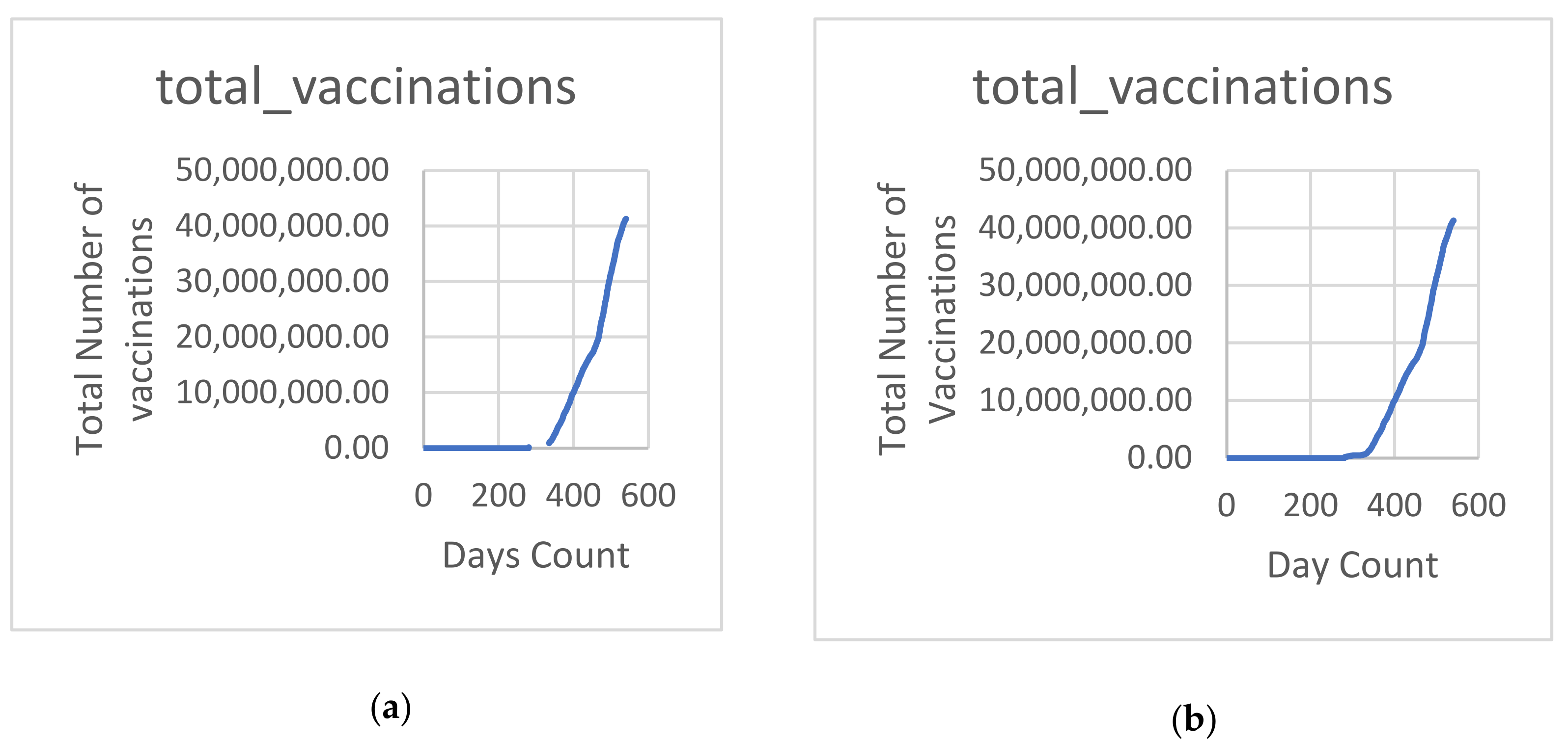
| total-vaccinations | 540 | 6,862,518 | 11,437,967 | 0 | 0 | 10,809,238 | 41,290,665 |
| stringency-index | 540 | 60.142 | 12.783 | 50 | 52.78 | 60.19 | 94.44 |
| VUN | 540 | 66.722 | 7.722 | 47.36 | 60.58 | 72.465 | 80.3 |
| VTI | 540 | 199.288 | 27.629 | 122.38 | 175.482 | 221.49 | 234.31 |
| VTV | 540 | 124.528 | 15.734 | 84.78 | 107.958 | 138.33 | 142.41 |
| MME | 540 | 1236.719 | 149.344 | 807.4 | 1119.5 | 1341.4 | 1457.5 |
| MMN | 540 | 600.966 | 75.567 | 386.1 | 540.325 | 653.8 | 704.7 |
| gold-price | 540 | 6814.958 | 309.29 | 5919.95 | 6556.3 | 7053.407 | 7752.23 |
| oil-prices | 540 | 52.933 | 16.372 | 9.12 | 41.34 | 68.73 | 78.34 |
| Variable Symbol | Oil Prices | Gold Prices | ||||||
|---|---|---|---|---|---|---|---|---|
| SS | MSE | F Value | p-Value | SS | MSE | F Value | p-Value | |
| TC | 97.27 | 97.27 | 19.27 | 1.45 × 10⁻⁵ | 27,824,836 | 27,824,836 | 1511 | 1.91 × 10−138 |
| NC | 2879.85 | 2879.85 | 570.56 | 3.37 × 10−79 | 211,353.5 | 211,353.5 | 11.48 | 0.0007 |
| NC_smoothed | 996.57 | 996.57 | 197.44 | 8.81 × 10−37 | 129,593.1 | 129,593.1 | 7.039 | 0.008 |
| TD | 90.75 | 90.75 | 17.98 | 2.77 × 10⁻⁵ | 6075.404 | 6075.404 | 0.33 | 0.565 |
| ND | 22.07 | 22.07 | 4.37 | 0.037 | 93.30752 | 93.30752 | 0.005 | 0.943 |
| ND_smoothed | 1229.91 | 1229.91 | 243.67 | 2.66 × 10−43 | 230,428.2 | 230,428.2 | 12.51 | 0.0004 |
| TC_per_million | 1370.09 | 1370.09 | 271.44 | 5.38 × 10−47 | 4677.894 | 4677.894 | 0.25 | 0.614 |
| NC_per_million | 0.54 | 0.54 | 0.11 | 0.743 | 542.2688 | 542.2688 | 0.029 | 0.863 |
| NC_smoothed_per_million | 32.67 | 32.67 | 6.47 | 0.011 | 7617.666 | 7617.666 | 0.41 | 0.520 |
| TD_per_million | 474.52 | 474.52 | 94.01 | 4.045 × 10⁻²⁰ | 150,517.9 | 150,517.9 | 8.17 | 0.004 |
| ND_per_million | 23.41 | 23.41 | 4.64 | 0.031 | 5520.553 | 5520.553 | 0.29 | 0.584 |
| ND_smoothed_per_million | 0.03 | 0.03 | 0.01 | 0.940 | 33,612.67 | 33,612.67 | 1.82 | 0.177 |
| reproduction_rate | 440.53 | 440.53 | 87.28 | 6.51 × 10⁻¹⁹ | 149,960.9 | 149,960.9 | 8.146 | 0.004 |
| NT | 110.80 | 110.80 | 21.95 | 3.82 × 10⁻⁶ | 686,444.9 | 686,444.9 | 37.29 | 2.397 |
| TT | 664.40 | 664.40 | 131.63 | 1.46 × 10⁻²⁶ | 6409.206 | 6409.206 | 0.34 | 0.555 |
| TT_per_thousand | 15.63 | 15.63 | 3.10 | 0.079 | 266,227.8 | 266,227.8 | 14.46 | 0.0001 |
| NT_per_thousand | 0.48 | 0.48 | 0.09 | 0.758 | 50,317.62 | 50,317.62 | 2.73 | 0.099 |
| NT_smoothed | 26.45 | 26.45 | 5.24 | 0.022 | 68,690.21 | 68,690.21 | 3.73 | 0.054 |
| NT_smoothed_per_thousand | 1.19 | 1.19 | 0.24 | 0.627 | 38,354.85 | 38,354.85 | 2.08 | 0.149 |
| positive_rate | 85.52 | 85.52 | 16.94 | 4.671 × 10⁻⁵ | 10,960.87 | 10,960.87 | 0.59 | 0.44 |
| tests_per_case | 6.72 | 6.72 | 1.33 | 0.249 | 130,501 | 130,501 | 7.089 | 0.008 |
| total_vaccinations | 556.24 | 556.24 | 110.20 | 5.95 × 10⁻²³ | 1,404,073 | 1,404,073 | 76.27 | 6.66 × 10⁻¹⁷ |
| stringency_index | 3.56 | 3.56 | 0.71 | 0.40 | 631,517.1 | 631,517.1 | 34.3 | 9.78 × 10⁻⁹ |
| VUN | 4.68 | 4.68 | 0.93 | 0.33 | 4290.694 | 4290.694 | 0.23 | 0.629 |
| VTI | 9.56 | 9.56 | 1.89 | 0.169 | 1,256,655 | 1,256,655 | 68.26 | 2.08 × 10⁻¹⁵ |
| VTV | 36.61 | 36.61 | 7.25 | 0.007 | 51,795.74 | 51,795.74 | 2.81 | 0.094 |
| MME | 31.10 | 31.10 | 6.16 | 0.013 | 1038.809 | 1038.809 | 0.05 | 0.81 |
| MMN | 19.89 | 19.89 | 3.94 | 0.0477 | 53,050.65 | 53,050.65 | 2.88 | 0.09 |
| Gold_price | 65.14 | 65.14 | 12.90 | 0.0003 | 237,554.9 | 237,554.9 | 12.9 | 0.0003 |
| Learning Parameters | Values |
|---|---|
| (Sparsity Proportion) | 0.05 |
| (Sparsity Regularization) | 4 |
| λ (coefficient of the weight regularizer) | 0.002 |
| No. of Epochs | 1000 |
| Oil Dataset | Gold Dataset | |||||
|---|---|---|---|---|---|---|
| Feature Selection Method | MSE | MAE | R Squared | MSE | MAE | R Squared |
| None | 1.5 × 10⁻² | 0.0628 | 0.993 | 2.13 × 10⁻¹ | 0.2575 | 0.909 |
| PCC Analysis | 1.23 × 10⁻² | 0.0583 | 0.994 | 1.13 × 10⁻¹ | 0.192 | 0.943 |
| Stacked Autoencoders | 2.019 × 10⁻² | 0.0865 | 0.989 | 2.357 × 10⁻¹ | 0.197 | 0.887 |
| Hybrid PCC- Stacked Autoencoders | 8.97 × 10⁻³ | 0.0476 | 0.995 | 5.356 × 10⁻² | 0.0951 | 0.973 |
| Publication | Method | Dataset | MSE | R Squared | MAE | RMSE |
|---|---|---|---|---|---|---|
| Yu et al. [37] | Support Vector Regression (SVR), ANN, and ARIMA | Crude Oil | - | - | - | 5.0493(ARIMA) 3.9337(SVR) 4.8682(ANN) |
| Xin James [48] | SVR, and ARIMA | Crude Oil prices | - | - | 1.1433(ARIMA) 1.1246(SVR) | - |
| Yan et al. [9] | De-dimension machine learning model using PCA, and RNN/LSTM approach to forecast the oil prices. | Crude Oil prices | - | - | 0.0844(RNN) 0.0905 (LSTM) 0.2784 (SVM) | - |
| Weng et al. [49] | Gold prices prediction using GA-ROSELM, genetic algorithm regularization online extreme learning machine | silver price, oil price, gold price | - | - | 5.681 | - |
| He et al. [50] | Denoising model to detect the noise factors in forecasting metal price using Multivariate Empirical Mode Decomposition | Silver, and gold prices | 1.222 | - | - | 1.105 |
| Khani et al. [51] | Encoder–decoder LSTM model for forecasting gold prices during the COVID-19 pandemic. | COVID-19 data records, and gold prices | 0.0217 | 0.858 | - | 0.147 |
| Jabeur et al. [52] | XGBoost machine learning approach for forecasting gold prices. | Metals, oil, and gold prices | - | 0.994 | 21.948 | - |
| Proposed framework | PCC-Stacked Autoencoder Hybrid feature extraction approach for forecasting the oil, and gold prices during the COVID-19 pandemic. | COVID-19 data records, oil, and gold prices | 0.0089 (oil) 0.0536 (gold) | 0.995 (oil) 0.973 (gold) | 0.0476 (oil) 0.0951 (gold) | 0.094 (oil) 0.231 (gold) |
Publisher’s Note: MDPI stays neutral with regard to jurisdictional claims in published maps and institutional affiliations. |
© 2022 by the authors. Licensee MDPI, Basel, Switzerland. This article is an open access article distributed under the terms and conditions of the Creative Commons Attribution (CC BY) license (https://creativecommons.org/licenses/by/4.0/).
Share and Cite
Samee, N.A.; Atteia, G.; Alkanhel, R.; Alhussan, A.A.; AlEisa, H.N. Hybrid Feature Reduction Using PCC-Stacked Autoencoders for Gold/Oil Prices Forecasting under COVID-19 Pandemic. Electronics 2022, 11, 991. https://doi.org/10.3390/electronics11070991
Samee NA, Atteia G, Alkanhel R, Alhussan AA, AlEisa HN. Hybrid Feature Reduction Using PCC-Stacked Autoencoders for Gold/Oil Prices Forecasting under COVID-19 Pandemic. Electronics. 2022; 11(7):991. https://doi.org/10.3390/electronics11070991
Chicago/Turabian StyleSamee, Nagwan Abdel, Ghada Atteia, Reem Alkanhel, Amel Ali Alhussan, and Hussah Nasser AlEisa. 2022. "Hybrid Feature Reduction Using PCC-Stacked Autoencoders for Gold/Oil Prices Forecasting under COVID-19 Pandemic" Electronics 11, no. 7: 991. https://doi.org/10.3390/electronics11070991
APA StyleSamee, N. A., Atteia, G., Alkanhel, R., Alhussan, A. A., & AlEisa, H. N. (2022). Hybrid Feature Reduction Using PCC-Stacked Autoencoders for Gold/Oil Prices Forecasting under COVID-19 Pandemic. Electronics, 11(7), 991. https://doi.org/10.3390/electronics11070991