SAGMAD—A Signature Agnostic Malware Detection System Based on Binary Visualisation and Fuzzy Sets

Abstract

Image conversion of byte-level data, or binary visualisation, is a relevant approach to security applications interested in malicious activity detection. However, in practice, binary visualisation has always been seen to have great limitations when dealing with large volumes of data, and would be a reluctant candidate as the core building block of an intrusion detection system (IDS). This is due to the requirements of computational time when processing the flow of byte data into image format. Machine intelligence solutions based on colour tone variations that are intended for pattern recognition would overtax the process. In this paper, we aim to solve this issue by proposing a fast binary visualisation method that uses Fuzzy Set theory and the H-indexing space filling curve. Our model can assign different colour tones on a byte, allowing it to be influenced by neighbouring byte values while preserving optimal locality indexing. With this work, we wish to establish the first steps in pursuit of a signature-free IDS. For our experiment, we used 5000 malicious and benign files of different sizes. Our methodology was tested on various platforms, including GRNET’s High-Performance Computing services. Further improvements in computation time allowed larger files to convert in roughly 0.5 s on a desktop environment. Its performance was also compared with existing machine learning-based detection applications that used traditional binary visualisation. Despite lack of optimal tuning, SAGMAD was able to achieve $91.94\%$ accuracy, $90.63\%$ precision, $92.7\%$ recall, and an F-score of $91.61\%$ on average when tested within previous binary visualisation applications and following their parameterisation scheme. The results exceeded malware file-based experiments and were similar to network intrusion applications. Overall, the results demonstrated here prove our method to be a promising mechanism for a fast AI-based signature-agnostic IDS.

1. Introduction

Today, there exists a variety of tools to protect computer systems and users from malicious activity. Intrusion detection systems (IDSs) are used as a protective mechanism by applying filtering techniques to distinguish between malicious and benign patterns. Current signature-based IDSs often fail to provide protection, as suspicious patterns need to be compared against a knowledge database that requires an ongoing update on the latest threats, for which no signature is available [1,2]. Due to the increasing sophistication of emerging cyber threats, researchers are now looking into signature-free IDSs for more promising results for the problem of zero-day threats [3]. Nevertheless, constructing a signature-free IDS presents a challenging problem, because mislabeled malicious activity could lead to an increase in false positives [4,5,6]. Consequently, there is a clear need to expand IDS performance to capture malicious patterns in an intelligent manner.

First, to tackle the problem of detecting unknown threats, we believe that binary visualisation can greatly assist in the construction of a signature-agnostic system [7]. Binary visualisation consists of converting a file into a pixelated image; this is achieved by taking the binary form of the file and converting it into a stream of pixel data before assembling it into a 2D structure [8]. In this way, suspicious code can become visible by forming unusual patterns of shape and colour [9]. Next, to achieve intelligent pattern detection of potentially malicious areas, we introduce the concept of colour value adaptation of the pixels based on fuzzy computations.

However, image conversion constitutes a computationally expensive process and additional costs based on machine intelligence methods will excessively increase running time and CPU [10,11]. As our research revolves around the construction of a system that analyses malware in real-time, it is important to address these limitations by concentrating our efforts on the optimisation of image conversion and effective pattern design processes.

To target these challenges, our paper presents the following contributions:

• We introduce SAGMAD, a binary visualisation tool that converts files into 2D images, based on the concept of capturing binary character similarities through Fuzzy Set theory. Our method was heavily based on binvis.io [12], a web application tool for security analysts which helps visualise binary file structures using the Hilbert curve clustering method.
• We employ an optimal clustering algorithm which has numerous advantages in terms of speed and byte representation intelligence. We also assess this method by measuring running time performance and comparing it with previous methods.

Ultimately, with SAGMAD, which can also serve as a potential tool for forensic and reverse engineering analysts, we aim to build a foundation algorithm that can serve as a real-time filtering method of a signature-free IDS in the future, and in this paper, we present the first step.

The remainder of this paper is divided into five sections. In Section 2, we provide an overview of the existing work on the field of binary visualisation, along with the evolution of binary visualisation tools. In Section 3, we present a binary visualisation methodology that uses an optimal space-filling curve and Fuzzy Set theory. In Section 4, we combine the results from the individual steps of our algorithm to evaluate its performance. In Section 5, we discuss our findings, along with their limitations and advantages. Finally, Section 6 concludes this paper and Section 7 outlines future work.

2. Related Work

2.1. The VizSec Domain, Works & Tools

In general, data visualisation plays an important role for successful detection in security operations. According to [8], visualisation for computer security (VizSec) is about “putting robust information visualization tools into the hands of humans to take advantage of the power of the human perceptual and cognitive processes in solving computer security problems”. VizSec methods can be distinguished into two broad categories: techniques for communicating value, and techniques for finding anomalies [13]. Our proposed methodology, SAGMAD, uses binvis.io, a 2D security tool that falls into the second category.

Recent academic work includes multiple malware detection methodologies that leverage visualisation techniques. For example, in [14], researchers concentrated their efforts on PE files using a navigational Hex editor and the Markov Byte Plot, a method that builds two 256 × 256 RGB representations of the file in order to detect packed portions. EventPad [15] is another promising tool which analyses PCAP files visually using automated rules. EventPad dissects network packets and represents them as series of blocks allowing for aggregation and selection in an effective and user-friendly GUI. Researchers in [16] proposed a signature-free framework, similar to SAGMAD in terms of image use and successful detection through supervised learning. More specifically, they focused on malware classification by building images of feature-based similarity matrices which are then used as input to several ML models for detection. More VizSec techniques and tools are reviewed by [17,18,19]. For a brief listing of 2D visualisation tools that are concentrated in network security only, the reader can consult the work of [20].

Recognising the effectiveness of 2D data visualisation methods in cyber security, Ref. [21] argues that newer technologies based on 3D representation of data, such as Virtual Reality, can drastically benefit Cyber Situational Awareness. Surprisingly, in their paper, Ref. [22] presented a 3D printed object called the Cr@ck3n, which acts as an alert in the case of a cyber attack communicating though light, sound, colour, and information scrolling.

2.2. Work & Tools Based on Binary Visualisation

Computer vision techniques focusing on byte-level analysis first made an appearance more than ten years ago, and several tools were proposed for successful structure analysis ever since. In his book in 2007, Ref. [23] was the first to introduce the concept of converting documents and images to graphical structures based on their ASCII characters. Later in 2008, joined by other researchers in [24], he demonstrated the “byte view” method as an extension to the existing research on hex editors to facilitate reverse engineering of files. They later extended their research on mapping byte plots and analysing different fragment types in [25,26].

Around the same time, several visualisation tools started to emerge from this research to help security professionals locate identifiable image patterns in files, such as CantorDust [27], Biteye & Vix [28], and Binary Analysis Tool [29]. For many of these tools, including the original “BinVis” tool by [24,30], development has now stopped or have reported bugs in their code. For others, development has been continued in different forms, like the recently presented CantorDust, which was reintroduced as a Ghidra plugin [31], or Binwalk Pro, a cloud version of the original Binwalk tool [32], which was recently acquired by Microsoft [33]. Experimentation on binary visualisation by Aldo Cortesi [34] started in 2011 and served as a precursor for binvis.io [12], which later became the main inspiration for Binspect [35], a Mac-based version of the application.

Binglide [36] is another interesting tool for reverse engineering that started as a master’s thesis drawing inspiration from previous tools. His creator later contributed to Veles [37], a mature version of it, published in 2016 for binary visualisation and analysis; Veles examines 2-grams and 3-grams of bytes and maps them into the 3D space to analyse their frequency and spatial distribution. Another tool is PortEx [38], which focuses on portable executables only.

2.3. Research Related to binvis.io

binvis.io was officially introduced in 2015 as a browser-based tool for visualising binary data that can also export images or particular segments for further analysis. However, the original code can also be downloaded from Github as a 2.7 Python package, called scurve [39]. scurve offers multiple visualisation options for investigating structural features of bytes, including different space-filling curves, as well as entropy visualisation serving as a measure of heterogeneity.

Even though the visual representation of computer files has been introduced as an effective countermeasure in malware analysis, according to our best knowledge there has been a limited number of studies based on the binvis.io tool.

Researchers in [40] used binvis.io to produce a dataset of images out of malicious and benign files, and train a self-organising neural network (SOINN) to evaluate it as a prediction mechanism. To achieve this, they extracted the prominent features of the generated images and used them as an input vector into the SOINN. The malicious files contained known malware classes and the algorithm achieved an overall detection rate of 74% when trained with optimal parameters. Another study published by [41] paired binvis.io image generation with several machine learning models to perform classification of known malware families. The model accuracy achieved a score of 91% under the k-nearest neighbours (KNN) algorithm and outperformed the work published in 2011 by [42] when tested at previously unknown files. We should note that even though [42] did not use binvis.io, they were the first to observe feature similarities of malware families in 2D grey scale images and were able to perform malware classification with 98% accuracy.

Malware Squid, proposed by [43], was a mechanism that used binary visualisation to propose a malware analysis of IoT network traffic. In this study, the authors presented a systematic approach to analyse real-time traffic data consisting of normal and malware traffic. Pcap file chunks were then collected and converted to 2D images that were processed by the MobileNet Convolutional Neural Network (CNN); the model was able to perform classification achieving an accuracy of 91%. An extension of the works of [40,43] was presented in [44], where the authors focused on training the Residual Neural Network (RNN) algorithm for a large number of malicious and legitimate pcap files. They achieved an overall accuracy rate of 94.5%.

2.4. Current Works with Image Conversion and Malware Detection

Current works that combine some form of pixelated image representation with machine learning models seem to successfully perform malware detection in a plethora of environments. Table 1 presents a summary of the most recent work in this domain. According to the summary, it is safe to say that the rise of deep learning (DL) and specifically visual imagery analysis networks have had a positive impact on image based malware detection and its performance rates. For example, Refs. [45,46], who both used colour, experimented with a large number of state-of-the-art DL models on Android and IoT datasets. Another factor for this tendency is the existence of several high quality datasets, such as the Malimg and the Leopard datasets, which provide a variety of file types for training and testing. Under this scope, it is worth mentioning that [47] curated a new dataset for malware detection, the Dumpware10 dataset, that resulted from their research.

We observe that all scientific work falls under two major goals: malware detection (distinction between malicious/benign files) and malware family classification; except for [48] who also performs family variant determination. This is independent from any type of environment, in other words, researchers are interested in detecting malicious activity on PCs, IoT, and mobile technology (Android and iOS) too. Ref. [49]’s work, which focused on IoT network traffic, involved the performance of dynamic analysis and image conversion on nested cloud environments and achieved excellent accuracy metrics for both known and new types of attacks.

In terms of data balance, there were works such as [50] where the numbers of samples were highly imbalanced. For others like [51], it was noted that despite the initial dataset being balanced, their approach was effective for imbalanced datasets too.

Following the recent rise in Generative adversarial networks (GANs) in image analysis, Ref. [52] used CycleGAN in order to increase the number of training examples, along with a diverse range of malware datasets that helped them achieve an accuracy of $99.87\%$. In [53], the authors leveraged the use of GANs to produce synthetic images of malware in order to make their method robust to malicious deformations.

Researchers have also started to take into account the use of colour, contrary to older methods that focused on gray scale representation of inputs. This was an effort to make the most of the RGB colour model, as colour images could carry more information in a relatively inexpensive way. For example, Ref. [54], who later extended their work in [55], had initially used grayscale images, and noticed that coloured images performed better in terms of accuracy, detection of obfuscated code, malware variant detection, and running times. Ref. [56] also experimented with gray/colour schemes and byte layout, such as the Hilbert space filling curve, with good results. Nevertheless, there exists no general effort from the research community towards experimentation with new colouring schemes or intelligent mapping of the byte sequence.

Older tools include a study by [57], who proposed a Java-based tool that used byte map, digraph, trigraph and histogram plot visualisations to label common file types. However, their experiment demonstrated several weaknesses and proved to be unreliable for prediction. For an extended review of various visualisation methods applied in malware analytics that were published before 2015, the reader is requested to consult the work of [58]. For a study on the effectiveness of recent image-based frameworks, the reader is requested to consult the work of [59].

Table 1. Summary of current works on general image-based malware detection.

Related Work	Year	Environment	Goal 1	Image Novelty	Colour Scheme	Dataset	Distribution	Models	Best Accuracy
[48]	2020	Mobile	(1), (2), (3)	No	Gray	Android apps, Apple apps	balanced	J48, RF, RT, BN, Ada Boost, DL	91.8% for Android, 96.4% for iOS
[46]	2020	IIoT	(1), (2)	No	Colour	Malimg, Leopard	imbalanced	DL (CNN)	98.47%
[49]	2020	IoT	(1)	No	Colour	IoT network traffic	imbalanced	DL (CNN)	99.28%
[54]	2020	PC	(2)	No	Gray	Malimg	imbalanced	DL (CNN)	99%
[60]	2020	IoT	(1)	No	Gray	Android apps	balanced	DL (CNN)	95.8%
[55]	2020	PC	(2)	No	Colour	Malimg, IoT-Android	imbalanced	DL (CNN)	98.82%
[56]	2020	PC	(1)	Yes	Colour	VirusShare, Windows 10	balanced	XGBoost, DL (CNN)	93.01%
[61]	2020	PC	(2)	No	Gray	Malimg	balanced and imbalanced	SVM, DT, KNN, DT, DL (CNN), etc.	99.3%
[62]	2021	PC	(1), (2)	No	Colour	Win-API call sequences	imbalanced	DL (CNN)	98%
[63]	2021	PC	(1)	No	Colour	Virussign, Windows 7	imbalanced	DL (CNN)	92.5%
[51]	2021	PC	(1), (2)	No	Gray	Malimg, Microsoft’s BIG 2015, MaleVis, Malicia, Windows	balanced	DL (CNN)	98.46%
[64]	2021	Android	(1), (2)	Yes	Colour	Android apps	imbalanced	DL (CNN)	97%
[50]	2021	PC	(1), (2)	No	Gray	Malimg	imbalanced	DL (CNN)	97.68%
[47]	2021	PC	(1), (2)	No	Gray	Dumpware10	imbalanced	J48, RBF, SMO, RF, XGBoost, SVM	96.39%
[45]	2022	Android	(1)	Yes	Colour	Leopard, Android apps	imbalanced	DL (CNN), SVM, RF	95.7%
[52]	2022	Mobile, PC	(1), (2)	No	Colour	Malimg, VirusShare, VirusTotal, Contagio	imbalanced	DL (CNN, RNN)	99.87%
[53]	2022	PC	(2)	No	Colour	Microsoft’s BIG 2015	imbalanced	DL (CNN, RNN)	97.47%

¹ (1) Detect maliciousness, (2) Malware family classification, (3) Family variant determination.

Table 1. Summary of current works on general image-based malware detection.

Related Work	Year	Environment	Goal 1	Image Novelty	Colour Scheme	Dataset	Distribution	Models	Best Accuracy
[48]	2020	Mobile	(1), (2), (3)	No	Gray	Android apps, Apple apps	balanced	J48, RF, RT, BN, Ada Boost, DL	91.8% for Android, 96.4% for iOS
[46]	2020	IIoT	(1), (2)	No	Colour	Malimg, Leopard	imbalanced	DL (CNN)	98.47%
[49]	2020	IoT	(1)	No	Colour	IoT network traffic	imbalanced	DL (CNN)	99.28%
[54]	2020	PC	(2)	No	Gray	Malimg	imbalanced	DL (CNN)	99%
[60]	2020	IoT	(1)	No	Gray	Android apps	balanced	DL (CNN)	95.8%
[55]	2020	PC	(2)	No	Colour	Malimg, IoT-Android	imbalanced	DL (CNN)	98.82%
[56]	2020	PC	(1)	Yes	Colour	VirusShare, Windows 10	balanced	XGBoost, DL (CNN)	93.01%
[61]	2020	PC	(2)	No	Gray	Malimg	balanced and imbalanced	SVM, DT, KNN, DT, DL (CNN), etc.	99.3%
[62]	2021	PC	(1), (2)	No	Colour	Win-API call sequences	imbalanced	DL (CNN)	98%
[63]	2021	PC	(1)	No	Colour	Virussign, Windows 7	imbalanced	DL (CNN)	92.5%
[51]	2021	PC	(1), (2)	No	Gray	Malimg, Microsoft’s BIG 2015, MaleVis, Malicia, Windows	balanced	DL (CNN)	98.46%
[64]	2021	Android	(1), (2)	Yes	Colour	Android apps	imbalanced	DL (CNN)	97%
[50]	2021	PC	(1), (2)	No	Gray	Malimg	imbalanced	DL (CNN)	97.68%
[47]	2021	PC	(1), (2)	No	Gray	Dumpware10	imbalanced	J48, RBF, SMO, RF, XGBoost, SVM	96.39%
[45]	2022	Android	(1)	Yes	Colour	Leopard, Android apps	imbalanced	DL (CNN), SVM, RF	95.7%
[52]	2022	Mobile, PC	(1), (2)	No	Colour	Malimg, VirusShare, VirusTotal, Contagio	imbalanced	DL (CNN, RNN)	99.87%
[53]	2022	PC	(2)	No	Colour	Microsoft’s BIG 2015	imbalanced	DL (CNN, RNN)	97.47%

¹ (1) Detect maliciousness, (2) Malware family classification, (3) Family variant determination.

2.5. Literature Review Conclusions and Motivation for This Work

Binary visualisation is not a new tool in the arsenal of security analysts. Nevertheless, since its conceptualisation in 2007 and its first use for malware family classification in 2011, there has been limited exploration of this method in terms of optimal image construction such as colouring schemes and information layout. Meanwhile, deep learning and image processing technologies have grown rapidly and have greatly improved malicious detection rates during the last few years. In our paper, we propose a novel method that leverages the binvis.io algorithm and fuzzy sets to assist pattern recognition before the images enter an ML/DL model. Under this scope, we believe that binary visualisation can be successfully employed to address issues in the development of signature-free IDSs, and in the next section, we will present our framework.

3. Materials and Methods

3.1. Building a Signature-Agnostic IDS Based on Binary Visualisation & Fuzzy Sets

In this section, we describe the construction of SAGMAD, a binary visualisation methodology based on the pre-existing binvis.io application. In the past, visualisation methods were used to reveal malicious activity by ensuring that all information is being captured (no area should be left untreated as per method) and that accurate detection would be the result of robust computational techniques (such as optimal representation of data in space or successful statistical analysis of treated data). However, we argue that there is much information to be derived from relations between data, since each element can simultaneously reveal trends for its environment too (information representation does not have to be one dimensional). Given that colour coding schemes are heavily underused in security applications, SAGMAD leverages an existing colour scheme to optimise its capabilities for more effective pattern recognition.

In this paper, we propose SAGMAD as the core element of a signature-free IDS, the development of which will come as a future extension to our current work. The IDS’s overall goal will be the detection of malicious activity in real-time after leveraging artificial intelligence algorithms. More specifically, a data set of files, labelled as malicious or benign, will be converted into binary images by our proposed methodology, the SAGMAD prototype, the full framework of which is explained in the following sections. Next, the 2D images will be provided into artificial intelligence algorithms for training and testing. The classified patterns will then be stored in a training database to serve the purpose of detecting previously unknown files in real-time. A visual depiction of SAGMAD as the building block of the IDS engine is shown in Figure 1.

To successfully construct SAGMAD, we first describe the individual parts that make it, starting from binvis.io and fuzzy set theory. We then describe SAGMAD’s colour computation and assignment method, before focusing on the clustering algorithm that optimally preserves the locality of the data as a sequence. We also provide details of the programming language and a description of the performance computing environments. Finally, to compare detection performance between SAGMAD and previous BinVis-based experiments, we provide a detailed analysis of the methodologies given in Section 2.3. To complete our proposed methodology, we evaluate the results by employing the most commonly used machine learning metrics, a full description of which is given in the last part of this section.

3.2. BinVis

binvis.io is a browser-based tool that converts files into 2D binary images. The binvis.io algorithm (“BinVis” from now on) sees files at the byte level and assigns a different colour to each ASCII character, according to its class. Three main classes divide the ASCII table, plus two special case characters reserved for the analysis, making a total of five groups to compare against each byte of the file.

The colours as per class are the following:

• blue for printable characters
• green for control characters
• red for extended characters
• black for the null character, or 0x00
• white for the non-breaking space, or 0xFF

BinVis then uses the Hilbert space-filling curve as its main clustering algorithm for the coloured byte string and converts it into a 2D image. The concept of space-filling curves was explored in the nineteenth century when mathematicians were interested in finding a mapping of a 1D line into the 2D unit space in a way that traversed the full range of it. The first space-filling curve was discovered and published by Italian mathematician Giuseppe Peano in 1890 in [65]. The Hilbert curve, a variation of the Peano curves, was published a year later in [66]. In general, the Hilbert curve is preferred over other space-filling curves in various applications because of its locality-preserving behaviour [67].

For our research and the need to have colours that can exhibit a wide range of shades, we replaced the white and black colour values of the original algorithm with yellow and grey values, respectively.

3.3. Fuzzy Sets and Fuzzy Inference Systems

Fuzzy Set theory was proposed by Lotfi Zadeh in 1965 as an extension to the classical set theory, in which elements are described by fuzzy numbers. Fuzzy logic was introduced to approach a more realistic way of human thinking in a way that could provide tools for dealing with vagueness and imprecision of data in decision making. In fuzzy logic, knowledge representation is “interpreted as a collection of elastic or, equivalently fuzzy constraint on a collection of variables [68]”. Consequently, “inference is viewed as a process of propagation of elastic constraints [68]”.

In fuzzy set theory, elements can belong to more than one fuzzy set, using the notion of set membership. These relations are represented by a degree of membership, and it describes the degree of truth of an element. According to [69], given a non-empty set X, a fuzzy set $\tilde{A}$ in X is characterized by a membership function ${\mu }_{\tilde{A}}$:

$${\mu }_{\tilde{A}}:X\to [0,1]$$

(1)

and it is described as set of ordered pairs $(x,{\mu }_{\tilde{A}}\left(x\right))$:

$$\tilde{A}=\{(x,{\mu }_{\tilde{A}}\left(x\right))|x\in X\}$$

(2)

where the first entity represents the element x of X, and the second one represents the membership value ${\mu }_{\tilde{A}}$ ranging from [0, 1]. This membership value defines the degree of membership of element x in the fuzzy set $\tilde{A}$ for each $x\in X$. In this way, a fuzzy set $\tilde{A}$ is defined by a set of tuples. It is worth noting that a membership value of 0 for an element would denote the complete non-membership of the element in the fuzzy set, whereas a value of 1 would represent full membership. Similarly, intermediate values ranging in $(0,1)$ represent a partial belonging of an element to a fuzzy set. Additionally, membership functions can take many shapes, such as triangular, trapezoidal, Gaussian, etc. Essentially, classical set theory is now considered a special case of fuzzy sets; a classical set is a fuzzy set whose membership value is either 0 or 1.

To capture the imprecision of data through natural language, Zadeh introduced the idea of linguistic variables in 1975, which was a core concept of fuzzy systems [70,71,72]. These are variables “whose values are not numbers but words or sentences in a natural or artificial language [70]”. According to him, linguistic variables are associated with fuzzy sets using adjectives and hedges [73]. A full description of a linguistic variable requires the quintuple:

$$\langle x,T\left(x\right),U,G,M\rangle$$

(3)

or the name x of the variable, the set of terms $T\left(x\right)$, the universe of discourse U, the syntactic grammar G, and the semantic rules M [70].

To introduce inference from linguistic variable operations, fuzzy logic uses a set of statements, called fuzzy rules, of the following structure:

“if <condition 1> and … and <condition k>, then <conclusion>”

where condition statements concern the input variables, conclusion statements concern the output variable/s and usually both take the form of “$x_i$ is $T\left(x_i\right)$” [74].

In general, there are three major types of fuzzy inference rules: the Mamdani fuzzy rules [75,76], the Takagi-Sugeno (TSK) fuzzy rules [77,78], and the Tsukamoto fuzzy rules [79], depending on the nature of <condition> and <conclusion>. In the Mamdani inference method, which is the most common one and can be found with multiple variations in literature, both <condition> and <conclusion> are fuzzy sets. In the TSK model, the output is a function of the input variable(s) and the idea is to generate the fuzzy rules based on an existing dataset of the dependent and independent variables. Lastly, in the Tsukamoto method, the output variable is a fuzzy set of a monotonic membership function.

Once all parameters for the inference model have been determined, e.g., type of the model, input/output variables, linguistic terms (or the fuzzy sets to be associated with them), fuzzy rules and shape of membership functions, the system is ready to accept crisp inputs and proceed to fuzzy operations that lead to intelligent decisions. This process is better known as a fuzzy inference system (FIS) and it is generally described by three main blocks:

• Fuzzification: Translate input into truth values.
• Evaluation: Compute output truth values.
• Defuzzification: Transfer truth values into output.

It is worth noting that both TSK and Tsukamoto models avoid the costly defuzzification computations that are present in the Mamdani method. This is achieved by the fact that the outputs of their fuzzy rules are crisp numbers, which in turns facilitates the aggregation computations during the defuzzification part of the FIS.

3.4. SAGMAD

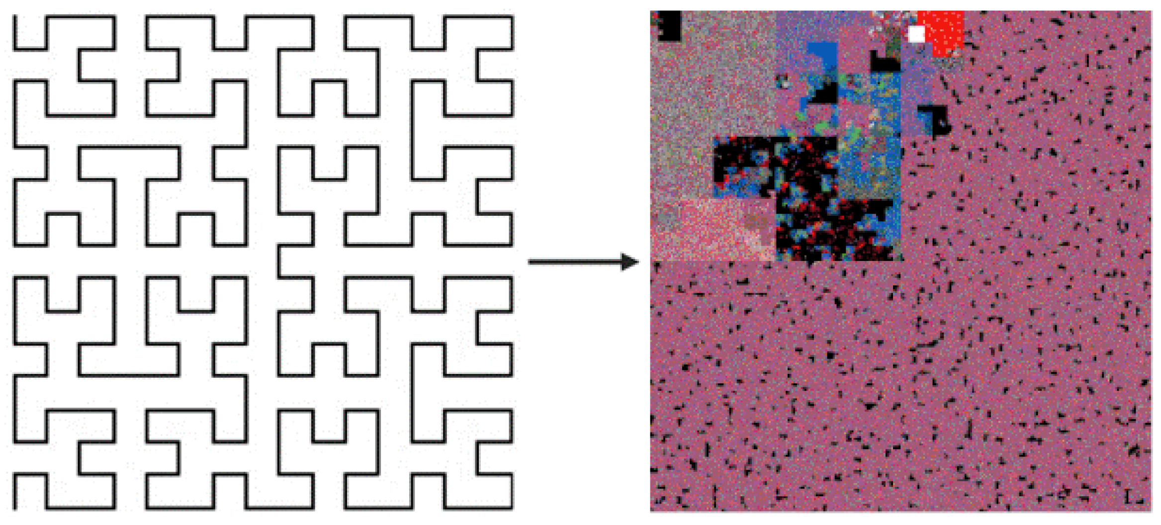
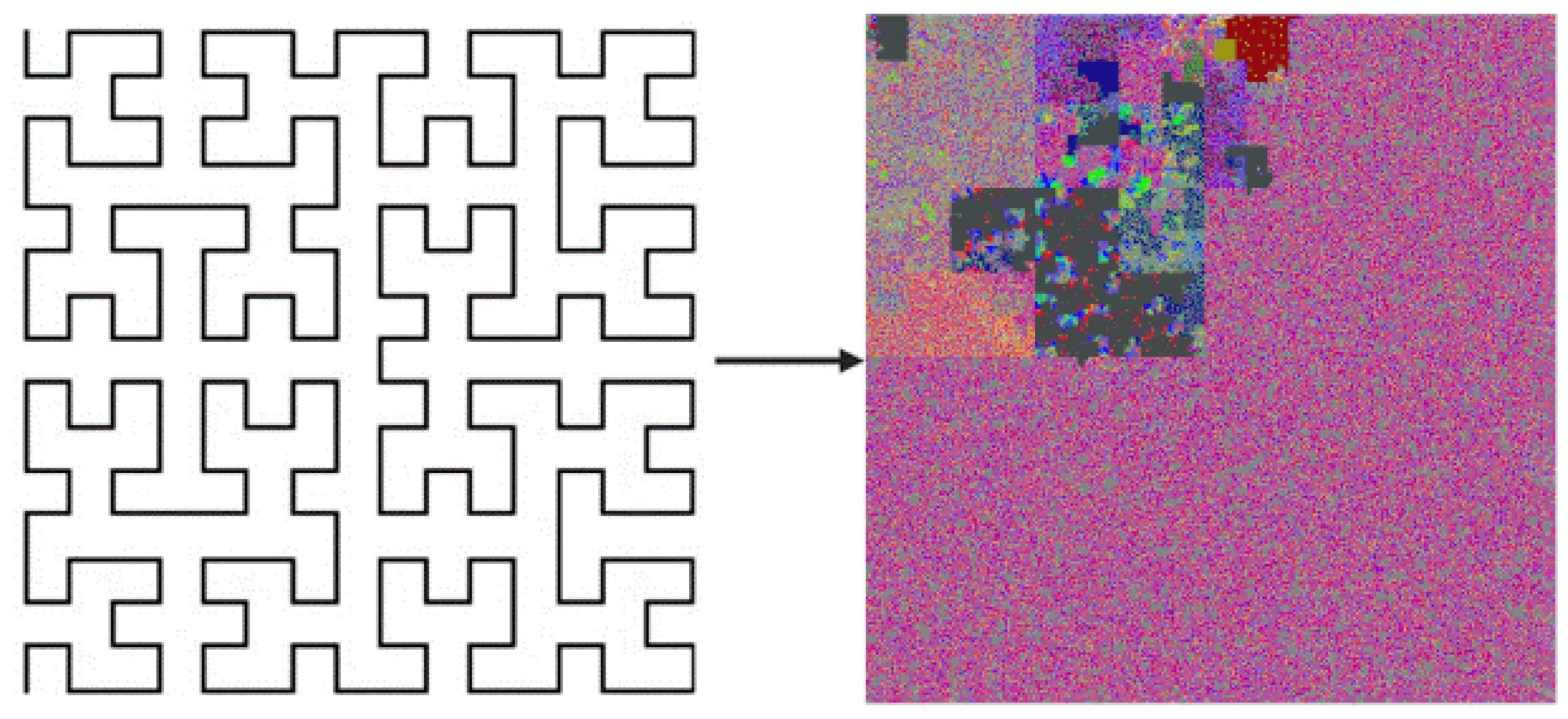
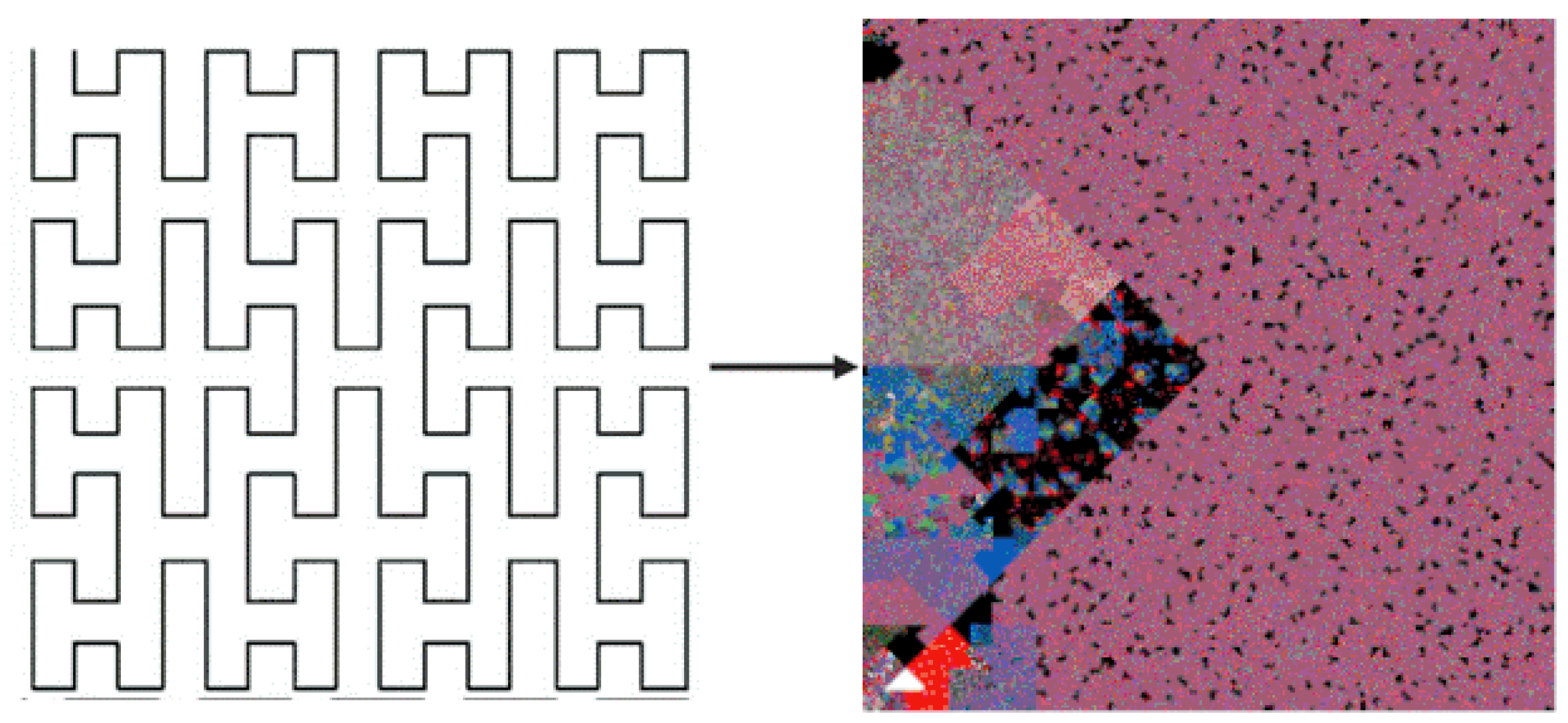
SAGMAD is a novel method based on the code provided by BinVis, that tries to intelligently capture byte sequence patterns through different tones of colour values. This is achieved by introducing the concept of colour tone to the already used colour value-as-per-class assignment.

According to our method, the colour tone of each byte is determined by the class types of its adjacent bytes. As previously discussed, BinVis assigns a colour value to each byte based on its ASCII value representation. In the case of SAGMAD, the colour assignment process remains the same, except that the algorithm is now evaluating a particular number of bytes that lay before and after the newly coloured pixel. It is worth noting that the algorithm sees the set of bytes arriving before the current byte and the set of bytes coming after it as two separate sets. It then continues by measuring the similarity of each collection to the current byte, with each similarity value contributing to its colour tone using fuzzy-based rules. In each case, the comparison of adjacent bytes is presented through the positioning of the array and before the space-filling clustering procedure is applied.

Essentially, SAGMAD adjusts the colour tone for each byte concerning whether n bytes located on either side of it belong to the same class, and assigns this value as a colour tint or shade. While BinVis tries to reveal patterns in code by visualising the byte class, the goal of SAGMAD is to make those areas stand out and facilitate image processing models. This is concerned with the fact that benign files appear to have a homogeneous distribution of printable (blue) and extended (red) ASCII characters, whereas malicious files present clustered areas of null (black) and orange (green) characters. In this way, broad homogeneous areas have their colour standards toned down, while “islands” of the malicious areas become more visible by becoming darker. With SAGMAD, each byte is currently affected by both its type and its environment.

To equate the set of bytes placed next (left or right-separate) to the byte to which we are assigning colour value and tone, we add the concept of similarity. We define the similarity as the ratio of the number of bytes within this set (left or right) that belong to the same class as the byte that we are currently interested in, over the total number of n bytes in the set.

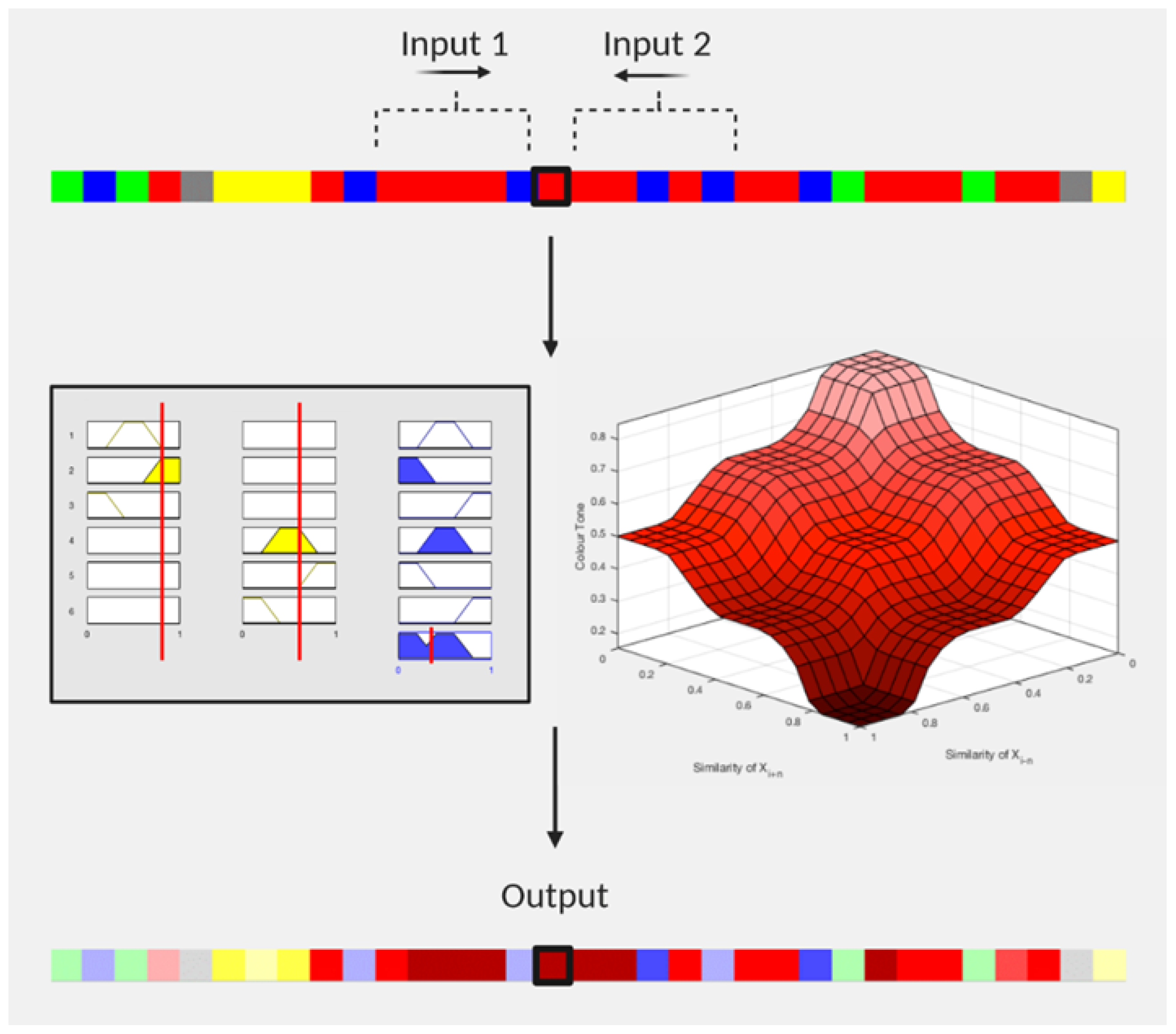
As illustrated in Figure 2, let us assume that we are involved in assigning colour value and tone to byte $x_i$, which is an extended ASCII character, and for which we consider five adjacent bytes per side, i.e., $n=5$. The byte is first given the red colour value and we begin to analyse the five bytes on each side to have its colour tone adjusted. On the left side, we find that four bytes out of the five are extended ASCII characters too, or, in other words, they belong in the “red” byte class as well, and calculate the similarity as $4/5=0.8$ (left similarity). In the same sense, we move on to the right side, counting once again the number of bytes that belong to the same class, and we find that three out of the five bytes are also in the red category. Hence, we measure a similarity of $3/5=0.6$ (right similarity). The two similarities are then given as inputs into a fuzzy inference system (FIS) where the colour tone is given as an output value of 0.35. As a result, the red (extended) character darkens because it resembles its environment. We should note that in the case of zero bytes belonging in the same byte class, the similarity would be 0. Accordingly, if all five bytes were in the “red” byte sequence, the similarity would be 1. It is a given that the colour adjustment of a red character will be within the red colour spectrum. The 3D shape in Figure 2 represents the whole spectrum of the potential red colour tones, ranging from 1 (the most pale) to 0 (the darkest) according to the membership functions of the FIS (we define this FIS later). The same reasoning follows the bytes of the example that had their colours toned down. As we observed in our example, we consider two sides per byte so that the tone is influenced by two measures of similarity. The number n, which specifies the number of objects we consider per collection, is always the same; in other words, we count the same number of bytes on the left and the same number of bytes on the right side of the byte $x_i$. Throughout the process, we keep $n=5$.

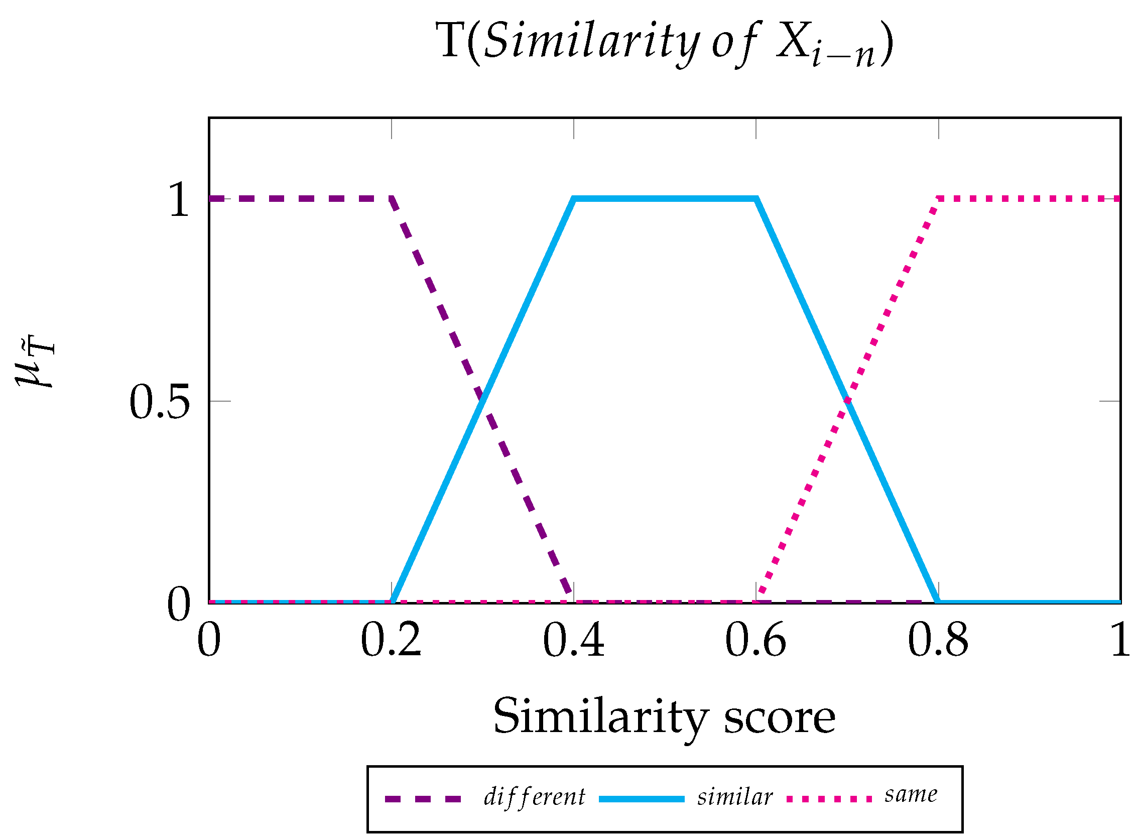
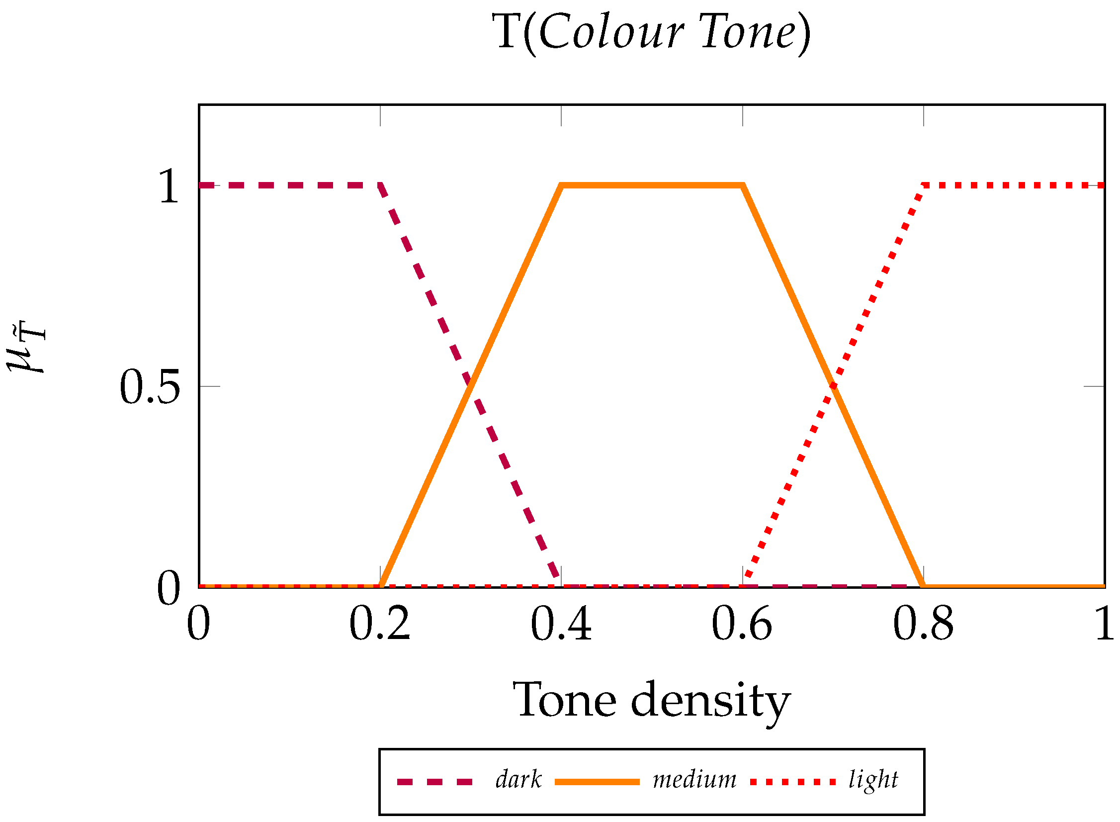
We now define the fuzzy inference system that determines the colour tone of the byte $x_i$, based on the two similarities that relate to it. For our process, we call $X_{i-n}$ the set of bytes on the left and $X_{i+n}$ the set of bytes on the right. To create the FIS, we use two input variables and one output variable, which are the linguistic variables of the scheme. We describe a set of values for each linguistic element, the Fuzzy Sets.

According to the above and the theory presented in Section 3.3, we define the linguistic variables and provide the visual representation in Figure 3, Figure 4 and Figure 5.

• Similarity of${\mathit{X}}_{\mathit{i}-\mathit{n}}$(left similarity):

Input variable. Linguistic variable values: Different, Similar, and Same.

• Similarity of${\mathit{X}}_{\mathit{i}+\mathit{n}}$(right similarity):

Input variable. Linguistic variable values: Different, Similar, and Same.

• Colour Tone:

Output variable. Linguistic variable values: Dark, Medium, and Light.

We also define the set of rules, which will constitute the machinery for the FIS.

  Fuzzy rules for $X_{i-n}$:

• IF Similarity of $X_{i-n}$ IS Different THEN Tone is Light.
• IF Similarity of $X_{i-n}$ IS Similar THEN Tone is Medium.
• IF Similarity of $X_{i-n}$ IS Same THEN Tone is Dark.

Fuzzy rules for $X_{i+n}$:

• IF Similarity of $X_{i+n}$ IS Different THEN Tone is Light.
• IF Similarity of $X_{i+n}$ IS Similar THEN Tone is Medium.
• IF Similarity of $X_{i+n}$ IS Same THEN Tone is Dark.

Essentially, by employing an FIS, we measure how much each similarity contributes to the tone of byte $x_i$. For instance, by examining how red byte $x_i$ should be, we ask what the degrees of truth are that byte $x_i$ belongs to the fuzzy sets Light, Medium, and Dark. As it was demonstrated in our example, the more a byte is surrounded by red class bytes, the darker it becomes. Similarly, bytes that find their surroundings dissimilar to them adopt pale tones.

To achieve the colour tone modification numerically, we pair the HSL (or Hue, Saturation, Lightness) colour model, firstly introduced in [80], along with the RGB model; we first keep the assigned RGB values intact as described in Section 3.2 to represent colors in their purest form. We then use HSL’s Lightness $L\in [0,1]$ to express the output FIS variable Colour Tone, without modifying Hue or Saturation. Shifting Lightness values towards 0 or 1, shifts a colour towards fully black or fully white, respectively.

Finally, for the formulation of the input/output mappings, we choose to apply the more intuitive Type-1 Mamdani FIS with the $min$ implication and $max$ aggregation methods. Then, to compute the output crisp value $z^{*}$ we use the centroid defuzzification method, given by:

$$z^{*}=\frac{{\sum }_i\mu \left(x_i\right)x_i}{{\sum }_i{x}_i}$$

(4)

where $\mu \left(x_i\right)$ is the membership value for point $x_i$ in the universe of discourse U.

3.5. The H-Curve Mapping

Preserving the locality for mesh indexing is of paramount importance to the efficiency of our data structure. This is also an especially crucial point for the next steps in our work, as more attempts will be made to achieve higher precision in the AI dimension of the IDS architecture.

To overcome this problem, we employed the H-curve algorithm, a 2D indexing scheme which was proposed by [81] and was first presented under the name “H-indexing”. The H-curve algorithm is made available in scurve [39] as one of the mapping layouts. By converting a file to an image based on this method, we achieve better locality preservation of our data than the widely used Hilbert curve indexing. This also holds truth for the Euclidean distance, as well as the maximum and the Manhattan metrics.

In general, in space-filling curves, the locality property is defined by a small constant c. For Hilbert, $c=\sqrt{6}$, while for the H-curve $c=2$. According to the H-curve method, the maximal distance between two mesh nodes, indexed i and j, is a slow-growing function of $|i-j|$. More specifically, the H-indexings form a Hamiltonian cycle that exhibits optimal locality-preserving among all cyclic indexings, as they provide tight lower bounds without any restriction. For a compact review of space-filling curves, the reader is invited to refer to [82]. Mappings of the Hilbert and the H-curve method paired with the traditional and the proposed colouring scheme can be seen in Figure 6, Figure 7, Figure 8 and Figure 9.

3.6. The Data Set

To accurately test the image generation limitations and constraints for each variation of the BinVis techniques outlined in this paper, we first required a collation of numerous file formats. For the construction of our data set, we acquired files from the Contagio dataset provided in [83], theZoo repository [84], the MalwareBazaar database in [85], as well as clean EXE files that were extracted from the base Windows Operating System. The final data set numbered a total of 5000 files that was averaged out in respect to their file sizes ranging from a few bytes to several megabytes in size. Its distribution can be seen in Figure 10. An enriched version of it has been uploaded and become available at the IEEE DataPort under DOI:10.21227/vs0r-8s26, along with the complete set of images that been created according to the described methodology.

3.7. Programming Language Selection for Image Generation

For performance purposes, we have opted to modify the programming language of the original method. As discussed earlier, the BinVis package was written in the Python programming language. To obtain quicker computational times, the paradigm has been translated to the Rust language [86]. Rust is a low-level language, best suited for low-level operating system interaction, embedded systems, and other improvements to memory management and code execution [87].

3.8. Image Generation in High Performance Computing & Desktop Environment

As discussed earlier, the original revisions to the BinVis [39] program showed significant flaws in the time of execution of the Hilbert image. This was evident for many phases of the algorithm, from raw data processing, to image creation and pixel positioning. As a result, this will cause a bottleneck when it comes to processing and generating vast volumes of real-time data.

To address this problem, we have implemented different hardware specifications to validate our methods by running our image conversion methods directly via the GPU. This was done by modifying the SAGMAD prototype to run parallel CUDA computing in Python (PyCUDA) [88] through the use of the GRNET High-Performance Computing Services [89]. GRNET HPC access permitted the allocation of batch jobs and allocated hardware access to 5000 GPU CUDA cores, allowing a significant reduction in computational load.

At the same time, the limitation of currently accessible data types in PyCUDA, such as the ability to transfer dictionaries and lists to the kernel for computing, did not enable certain functions to be completely configured for GPU processing. As a result, we used Just-in-Time Compilation (JIT) [90] in cases where CUDA optimization in GPU performance was not feasible.

For comparative purposes, we have also used a desktop environment to test the output of each process with the following hardware specifications:

• 16 GB RAM
• 4 Core CPU
• Intel integrated GPU

3.9. Machine Learning Metrics

To evaluate the contribution of SAGMAD towards accurate predictions of malicious patterns in unknown files, we will run the same machine learning algorithms that have been used in BinVis applications. The details of these experiments are discussed in Section 3.10.

As in all mathematical learning methodologies, some output indicators help to determine the robustness of the model. At the same time, when we want to assess SAGMAD using the best-performing machine learning techniques of previous research projects, we can also evaluate the findings using the same criteria to allow for a similar comparison.

For this purpose, we employ the accuracy, precision, recall, and F-score functions. To explain what these terms stand for, we first need to describe the individual values that make them, namely the True Positive ($TP$), True Negative ($TN$), False Positive ($FP$), and False Negative ($FN$) measures:

• TP is equivalent to all elements of a class that the algorithm correctly predicted to belong in that class. In other words, it is the number of malicious files correctly identified as malicious.
• TN is equivalent to all elements outside of a class that the algorithm correctly predicted to belong in a different class. In other words, it is the number of benign files correctly identified as benign.
• FP is equivalent to all elements outside of a class that the algorithm has incorrectly predicted to belong in that class. In other words, it is the number of benign files incorrectly identified as malicious.
• FN is equivalent to all elements of a class that the algorithm has incorrectly predicted to belong in a different class. In other words, it is the number of malicious files incorrectly identified as benign.

Next, we define the $Accuracy$, $Precision$, $Recall$, and $F\text{-}score$ metrics:

• Accuracy is the ratio of instances that were correctly predicted, or the ratio of the total hits (malicious and benign) of the algorithm. We provide the formula as:

  $$Accuracy=\frac{TP+TN}{TP+TN+FP+FN}$$

  (5)
• Precision is the proportion of correct predictions of malicious cases over the total amount of predicted malicious cases, or the ratio of actual malicious cases from all cases predicted as malicious. We provide the formula as:

  $$Precision=\frac{TP}{TP+FP}$$

  (6)
• Recall is the proportion of correct predictions of malicious cases over the total amount of malicious cases, or the percentage of malicious cases detected. We provide the formula as:

  $$Recall=\frac{TP}{TP+FN}$$

  (7)
• F-score is the harmonic mean between precision and recall, and is indicative of the accuracy and robustness of the model. We provide the formula as:

  $$F\text{-}score=\frac{2TP}{2TP+FP+FN}$$

  (8)

3.10. Comparison with Previous Applications Based on BinVis

To properly analyse the efficiency of SAGMAD over the original BinVis tool, we need to do a comparative analysis against current BinVis methods. These experiments were originally mentioned in Section 2. In their approach, the authors [40,41,43,44] used the BinVis algorithm to generate images which are used as input to the objective of feature classification. Their aim was to conduct either malware/benign filetype classification [40], malware family classification [41], or malware/benign IoT traffic classification [43,44].

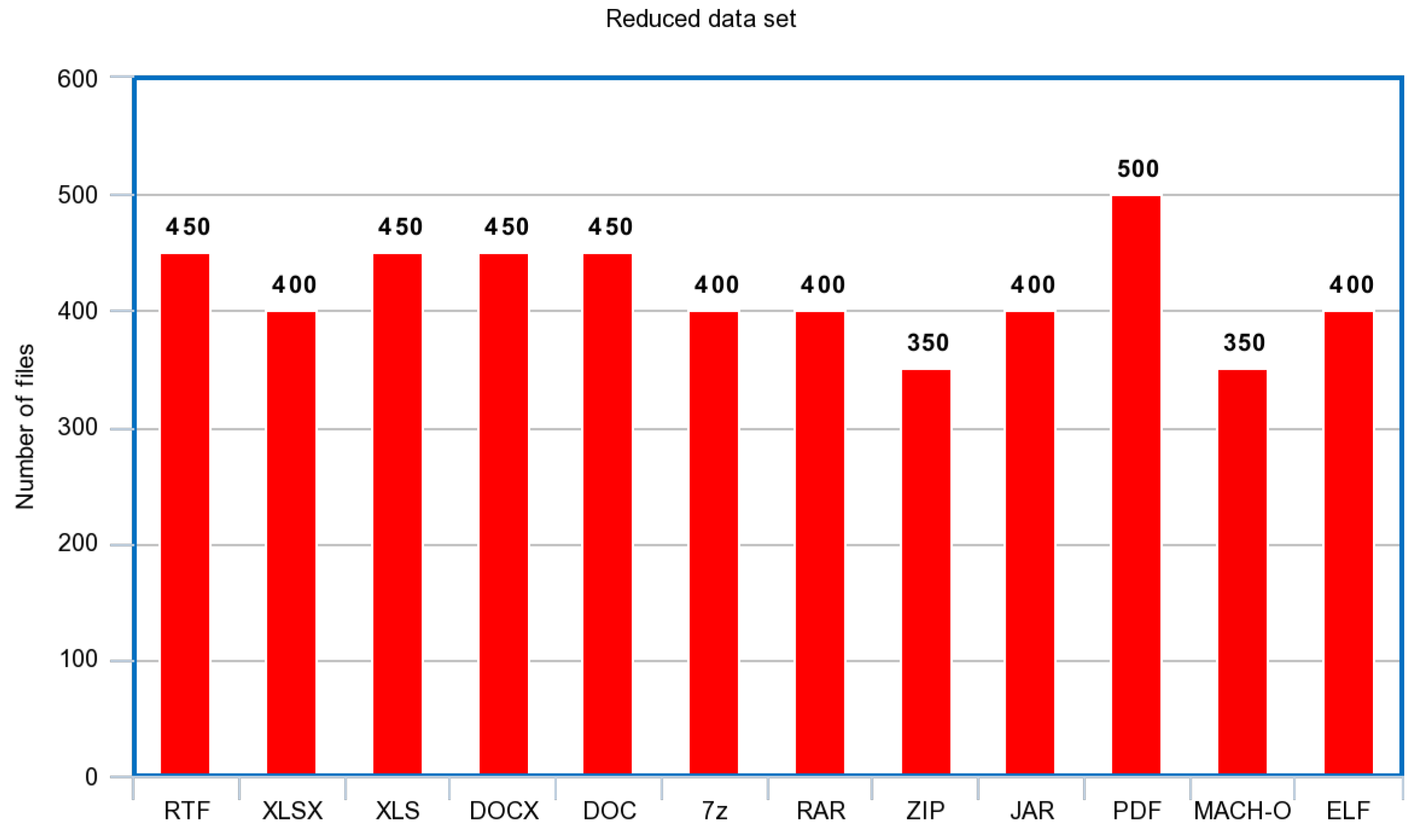
In the next paragraphs, we will briefly present their top-performing solutions and explain the technical aspects of their approaches. This research will serve as the basic model requirements when comparing the classification output of the images provided by BinVis and SAGMAD.

3.10.1. Baptista et al.’s Experiment

Image classification through machine learning methods is a powerful technique for computers to recognize patterns, especially when paired with neural networks. To perform detection of malicious activity among various file types, Ref. [40] employed a self organising incremental neural network (SOINN), a sophisticated neural network that uses only two layers. SOINN, which was initially proposed in [91], adopts a minimalist approach that keeps computational costs at a minimum without undermining its ability to perform successful pattern recognition. The two layers focus on mapping a topological structure of the input data competitively while taking on different tasks. The first layer estimates the density distribution of the input vector by selecting a first and a second winner, and builds an undirected graph representation that is continuously being improved. The second layer can detect the different clusters by looking at the low-density areas between them. Many improved methods of SOINN have been proposed since its conception.

Regarding the construction of the feature vector, Ref. [40] recognised the spatial distribution of malicious patterns in specific parts of the binary representation of a file, particularly on the top and the bottom of the image, and divided the clustered image into four parts; top, bottom, upper and lower middle. This was particularly important since they included multiple malware types within the infected files of their data set. In the feature vector, each of these areas was represented by a vector of length 256 to denote the histogram of the RGB colour space. Regional feature vectors were then put together following the corresponding order of the regions in the image, resulting in a feature vector of length 1024. It should be noted that while SOINN is a robust algorithm for unsupervised learning, parameterisation should be handled with care. Ref. [40] was able to achieve an accuracy of 73.7% with 12% false positives and 14% false negatives for the overall malicious/benign file detection, with parameters lambda $\lambda$ = 290 (number of iterations) and max. age A = 170 (age of communicating nodes). For this experiment, the rectangle-shaped image of the scurve module was used.

3.10.2. O’Shaughnessy’s Experiment

Ref. [41] recognized the need for AV programs to perform malware family classification, and employed computer vision techniques to provide a scalable solution. For this reason, he performed data conversion while experimenting with three factors of the image conversion and classification process: a variety of space-filling curves, different feature extraction techniques, and various statistical learning models. Ref. [41] was the only one to try multiple space-filling curves offered by the scurve module, other than the more widely used Hilbert curve; namely the Z-order, Gray-code, and the Hilbert curve mappings were employed, offering different representations for the same malicious file contents. Images were then given as input to models using the local binary patterns (LBP), Gabor filters and histogram of gradients (HOG). After malware family names were paired with the appropriate feature vector, Ref. [41] tested three supervised machine learning algorithms, namely k-nearest neighbours (KNN), random forest (RF), and decision trees (DT).

Parameterisation has performed automatically for each model with the help of a Python module to evaluate the best parameter values. Out of all possible combinations, the best performing process proved to be the KNN-HOG Z-order model. The HOG method requires the tuning of various parameters, for which the author determined the best performance under orientation = 16, pixels-per-cell = 60 and cells-per-block = 1. To deal with changes in colour intensity, the L2-Hys normalisation was performed. Moving to KNN parameters, the number of neighbours was chosen to be k = 1, and the distance metric was the “cityblock” function. During the testing of the KNN-HOG Z-order method on unseen data, the model generalized well, with 82% precision, 80% recall, and 83% accuracy scores. It is important to note that for this experiment, the square-shaped image of the scurve module was used.

3.10.3. Shire et al.’s Experiment

IoT network traffic was monitored and cut in chunks by [43] in an attempt to identify potential malware traffic from smart devices. Network traffic was collected in the form of .pcap files, which were then converted into 2D binary visualisations. The overall idea of the experiment was to test the model on various malicious network traffic scenarios, such as DDoS, botnet, trojan horse traffic, alongside normal traffic, and test if binary visualization was a promising solution on the getaway level of connected devices.

In this problem, the researchers chose convolutional neural networks (CNN) as the primary detection algorithm. More specifically, they used Tensorflow’s MobileNet module, where the data were trained for 500 batches. The PCAP files were inserted into the CNN by dividing each image into smaller tiles.

In the test that used the largest number of samples, they were able to achieve the highest values for the following metrics: 91.32% accuracy, 91.67% precision, 91.03% recall, and 91.35% F-score. In this experiment, the researchers performed their method on the rectangular layout of the scurve module.

3.10.4. Bendiab at al.’s Experiment

Continuing the works of [40,43,44], the use of deep learning for classifying malicious/benign network traffic was proposed. Their best performing experiment employed the ResNet50 model, a CNN with 50 layers.

Their method tested 2D images of IoT traffic that represented a plethora of common attacks, such as DDoS, key loggers, back doors, and OS scans. For the training, the researchers iterated the model for 50 epochs with a batch size of six. They also incorporated the LRFinder function, a Python module that investigates the performance and finds the optimal parameters. According to this experimentation, they used a learning rate of 0.05.

Overall, deep learning outperformed previous efforts for classification; the experiment achieved 94.5% accuracy, 95.78% precision, 94.02% recall, and an F-score of 94.9%. Ref. [44] used the rectangular-shaped form to construct the image samples.

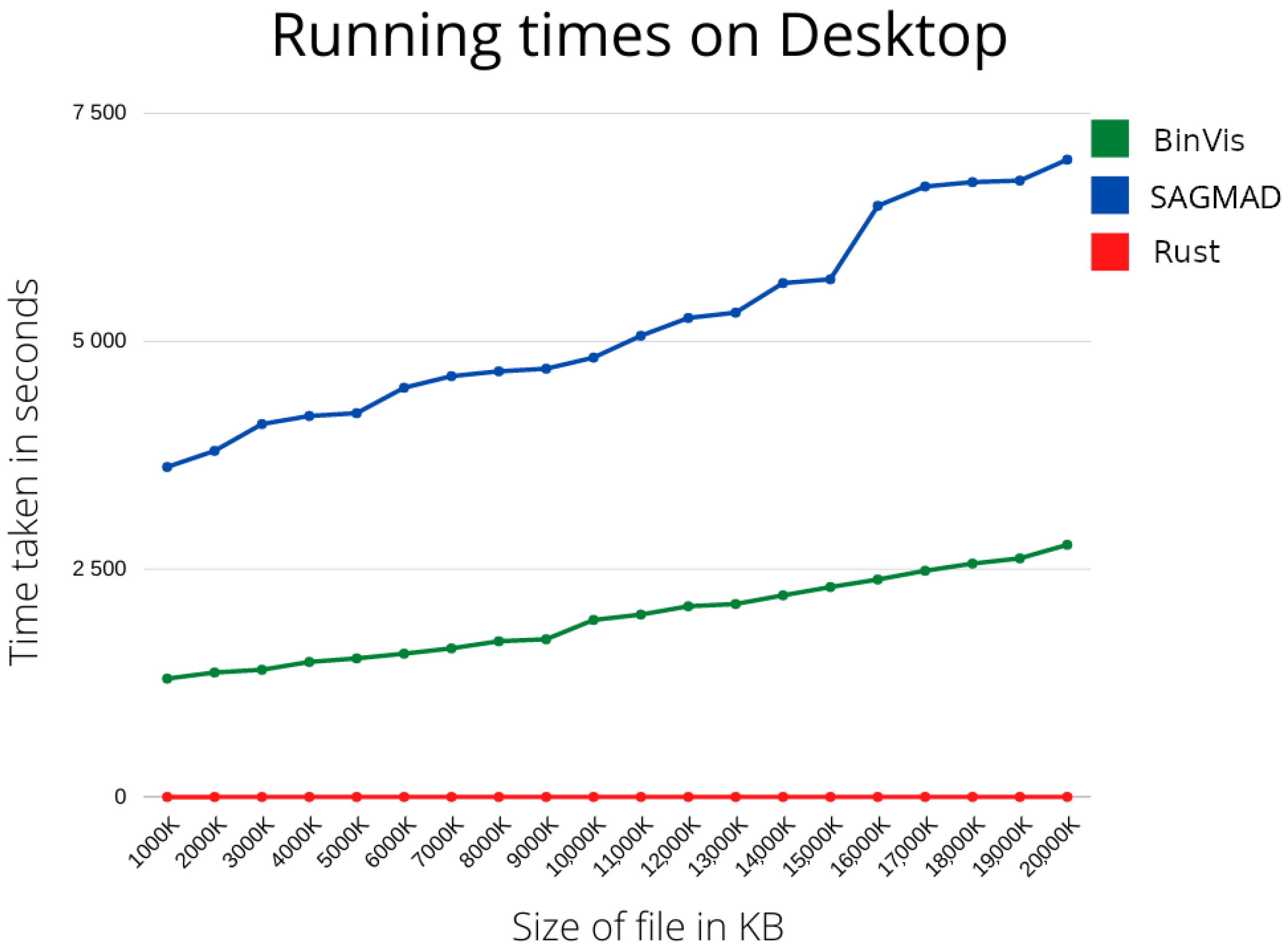
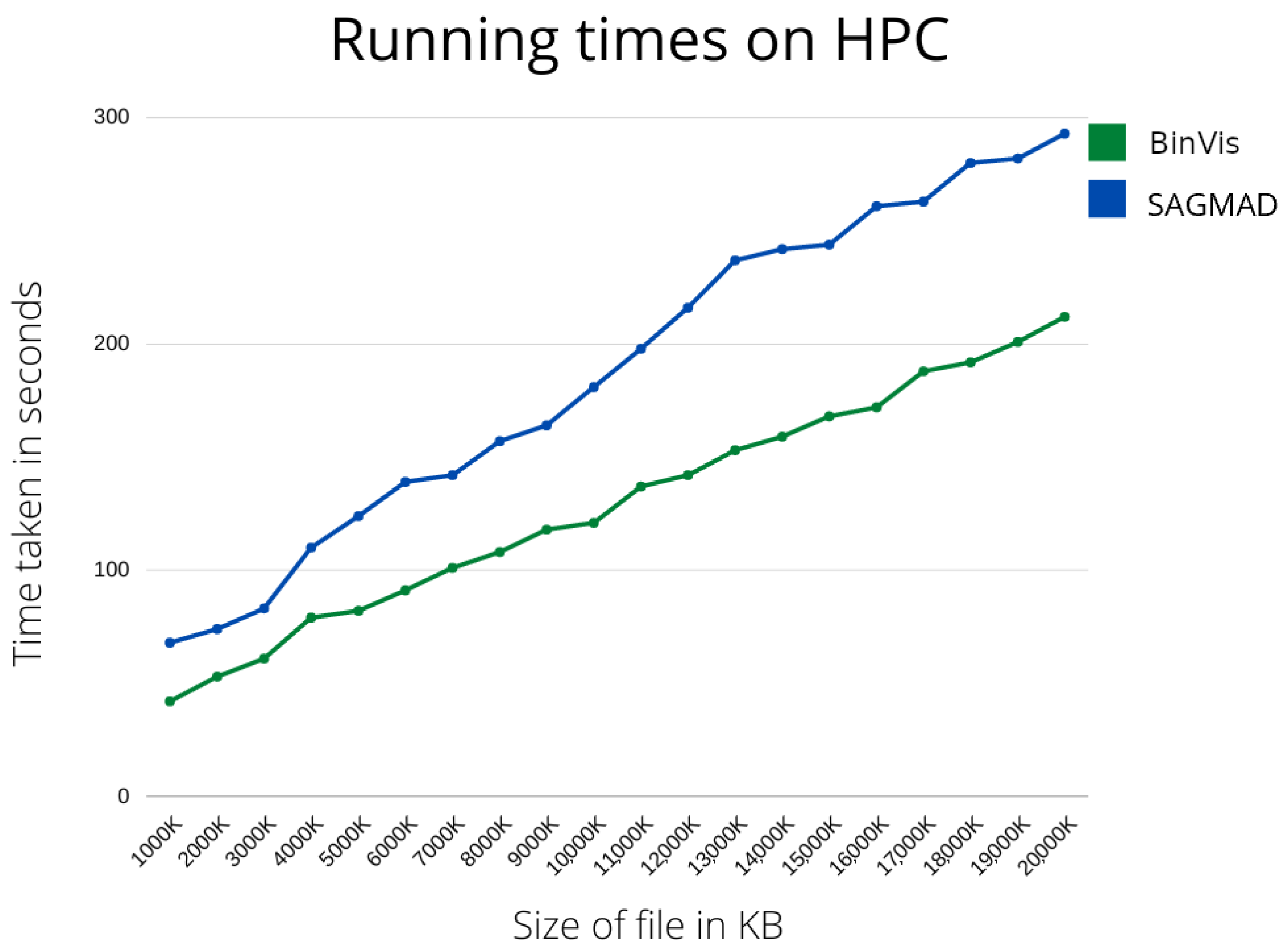
As previously stated, the main focus of our research has been the construction of a real-time malware detection system. In the next section, we are going to present the running times of our method and of the original package tested in different environments, as well as machine learning metrics to allow comparison with existing methods.

3.11. Programming Language Selection for Machine Learning Models

The Resnet50, SOINN, KNN-HOG and MobileNet learning algorithms were implemented using the open-source TensorFlow and Keras Python libraries in an Anaconda environment, utilizing NVIDIA driver 460, CUDA 10-1 and CuDNN 7.

3.12. Machine Learning Running Environment

The experiments were conducted on a physical machine, running on an AMD Ryzen 7 4800H 8 CPU Cores, 16 threads at 2.9 GHz with 64 GB memory running an Ubuntu 20.04 OS and an NVIDIA GTX 1660 Ti GPU with 6 GB memory was used as an accelerator.

4. Results

4.1. Image Generation Performance

In this section, we present the performance analysis results of our methodology that was implemented as described in Section 3. We first outline the results regarding the image generation part of our analysis, where we converted files into 2D representations based on a fuzzy logic color scheme of their ASCII characters. The specific methods and tools for this part were provided in Section 3.1, Section 3.2, Section 3.3, Section 3.4, Section 3.5, Section 3.6, Section 3.7 and Section 3.8.

To evaluate and compare the performance for the original BinVis algorithm and the proposed method, we measured the required length of time to generate images from the aforementioned data set in an increased file size arrangement. Initially, the file sizes in our compiled data set, which ranged from a couple of bytes to little over 20 MB in size, consisted of a large number of repeating common file sizes that would affect the evaluation of the methodologies. In order to clearly determine the efficiency in image generation, we decided to reduce the data set and focus on variation in computations instead. This was achieved by selecting a smaller set of files with exponential growth in their size.

As mentioned in previous Sections, the initial implementation steps and testing of our method proved to be a costly process, for which we needed to make use of an HPC infrastructure. Regarding the running times of the original BinVis algorithm on GRNET’s ARIS, incremental processing of file sizes ranging from 1000 KB to 20,000 KB was completed between the ranges of 52.356 s to 210.489 s. At the same time, when testing the performance of the Hilbert-curve SAGMAD method on ARIS, we achieved running times that ranged from 64.83 s to 284.63 s for the same range of file sizes. As it can be seen from these numbers, it is important to note that our access to high performing computers provided us great flexibility to test our methods regarding the colouring scheme and curve experimentation. By repeating the same experiment on a desktop computer, we acquired a range of 1299.9 to 2661.9 s for the BinVis implementation, and a range of 3623.99 to 7085.91 s of the Hilbert-curve SAGMAD method, an apparent limitation, not only for building and testing code, but for the construction of an IDS application running in real time.

Moving on to our final implementation, which employed the optimal locality-preserving H-curve written in Rust, the H-curve SAGMAD exhibited running times of 0.002 to 0.574 s on a desktop environment, again, for an incremental processing of file sizes from 1000 KB up to 20,000 KB. H-curve SAGMAD outperformed every binary visualisation technique, proving to be the best candidate for a real-time IDS traffic processing. For comparison reasons, we also run the original Hilbert-curve BinVis in Rust, which achieved running times of 0.001 to 0.512 s on a desktop environment, again, for an incremental processing of file sizes from 1000 KB up to 20,000 KB.

The full description of the running times per file size for desktop and HPC environments is shown in Figure 11 and Figure 12, respectively.

4.2. Performance of H-Curve SAGMAD within Machine Learning Algorithms

In this section, we present the performance of previously implemented binary visualisation applications when incorporated with SAGMAD images in their detection algorithm, the full description of which can be found in Section 3.9, Section 3.10, Section 3.11 and Section 3.12. More specifically, the detailed parametarisation and deliveries of these studies were presented in Section 3.10, while the notions of the various metrics for a machine learning based IDS were provided in Section 3.9. The methods described in these studies were recreated as faithfully as possible to match the original work of their researchers, while the goal was to replace the images implemented for detection with SAGMAD clustering.

Under this scope, we present the comparative performance between Hilbert BinVis and H-curve SAGMAD colouring schemes in

Table 2. Performance comparison with [41].

	KNN-HOG
	Accuracy	Precision	Recall	F-Score
Z-order BinVis	83.00%	82.00%	80.00%	80.99%
H-curve SAGMAD	91.83%	89.33%	94.32%	91.76%

,

Table 3. Performance comparison with [40].

	SOINN-RGB Histogram
	Accuracy	Precision	Recall	F-Score
Hilbert BinVis	73.70%	87.76%	86.00%	86.87%
H-curve SAGMAD	92.52%	87.90%	94.24%	90.96%

,

Table 4. Performance comparison with [43].

	MobileNet
	Accuracy	Precision	Recall	F-Score
Hilbert BinVis	91.32%	91.67%	91.03%	91.35%
H-curve SAGMAD	90.71%	91.33%	90.24%	90.78%

and

Table 5. Performance comparison with [44].

	ResNet 50
	Accuracy	Precision	Recall	F-Score
Hilbert BinVis	94.50%	95.78%	94.02%	94.90%
H-curve SAGMAD	92.68%	93.96%	91.98%	92.96%

when measured for accuracy, precision, recall and the F-score. We should note that for the replication of experiments run by [43,44], we rerun the their original methods (Hilbert BinVis with respective learning algorithms) using the malicious/benign file images produced by the data set in Section 3.6. This was an essential step to ensure that the comparison of metrics in Table 4 and Table 5 would concern images created from the same data type. Hilbert BinVis metrics in Table 2 and Table 3 on the other hand, were left the same.

The planned comparisons showed that SAGMAD outperformed the visualisation methods in KNN-HOG [41] and SOINN-RGB Histogram [40]. More specifically, SAGMAD delivered 91.83% accuracy, 89.33% precision, 94.32% recall, and an F-score of 91.76% when used with the KNN-HOG learning algorithm, and 92.52% accuracy, 87.90% precision, 94.24% recall, and an F-score of 90.96% when used with the SOINN-RGB Histogram model. Additionally, it exhibited similar performance when paired with MobileNet [43], achieving 90.71% accuracy, 91.33% precision, 90.24% recall and 90.78% for the F-score. At the same time, it exhibited slightly poorer results when incorporated in ResNet 50 [44], reaching 92.68% accuracy, 93.96% precision, 91.98% recall, and an F-score of 92.96%.

In

Table 6. Confusion matrix for the KNN-HOG experiment.

	Predicted
	Malicious	Benign
Actual
Malicious	2358 (TP)	142 (FN)
Benign	282 (FP)	2218 (TN)

,

Table 7. Confusion matrix for the SOINN-RGB Histogram experiment.

	Predicted
	Malicious	Benign
Actual
Malicious	2356 (TP)	144 (FN)
Benign	324 (FP)	2176 (TN)

,

Table 8. Confusion matrix for the MobileNet experiment.

	Predicted
	Malicious	Benign
Actual
Malicious	2256 (TP)	244 (FN)
Benign	214 (FP)	2286 (TN)

and

Table 9. Confusion matrix for the ResNet 50 experiment.

	Predicted
	Malicious	Benign
Actual
Malicious	2300 (TP)	200 (FN)
Benign	148 (FP)	2352 (TN)

, we also present the confusion matrices of our experiments as a performance measurement of the four different combinations of predicted and actual malicious/benign files.

5. Discussion

The results demonstrated in Section 4 represent the first efforts of our research towards the construction of signature-free IDS architecture. For this reason, measuring running time performance was one of the most important aspects of our method, given the interest in analysing excessive amounts of data in real-time. At the same time, our efforts focused specifically on optimal image construction and malware detection, with no effort being made towards optimising the machine learning part of the framework.

As is demonstrated in Figure 11, the performance analysis of the BinVis model in a desktop environment exhibited high running times even for small files, rendering it an unsuitable foundation algorithm for a real-time detection mechanism. On the other hand, even though computational functions were handled with great care within the first SAGMAD implementation, fuzzy-based operations heavily affected the running costs; the Hilbert SAGMAD method running times were about 2.7 times higher than the traditional BinVis. This limitation is also reflected on the lack of experimentation regarding the number n. Initial attempts to insert a larger number of adjacent bytes proved to be prohibitive during the early phases of the experiment and we eventually kept n as a constant to focus on code execution and malicious detection performance.

Further adaptation of the Hilbert curve SAGMAD on HPC (Figure 12) provided flexibility and experimentation with the method as computation times dropped 55 times for the smallest files, and 24 times for the largest ones compared to the Desktop application. Given the low running times from working on HPC, we were able to perform further improvements to optimisation, and proceeded with the implementation of the H-curve clustering method, as well as the conversion to Rust. The obtained results indicated the success of the method by dramatically decreasing running times, as shown in Figure 11. Due to these improvements in computation times, we were able to maintain high performance, with the largest file sizes converting in roughly 0.5 s. This is particularly important as it was achieved without trading off the time taken for image generation, even when working from a desktop CPU.

Given the results of the first part of our experiment, we can safely claim that we have eliminated the need for GPU assistance in generating binary visualisation images. These findings confirm our initial hypothesis and suggest that our method is able to perform file-to-image conversion and colour value computations for real-time data streams.

Moving on to the results produced for the second part of our methodology, and presented in Table 2, Table 3, Table 4, Table 5, Table 6, Table 7, Table 8 and Table 9, SAGMAD exhibited a consistent behavior in detecting malicious content when inserted in machine learning systems. It is important to note that these results were yielded when using the fuzzy-generated images within algorithms and parameters that were not tuned for the model’s optimal performance. By contrast, the execution of the experiment followed the feature extraction and the best-performing parameters that were investigated from the previous machine learning applications (see experiments in Section 3.10). Moreover, those applications incorporated training and testing data sets that exhibited quantifiable differences in affecting learning rates.

It is also important to emphasise the performance of the experiments given the small size of our dataset. One of the main goals of our paper was a ML framework where the training is performed fast. For this reason, we chose to employ a relatively small number of files with a diverse range of file sizes. This helped us to achieve a good performance and show that the learning rate could keep increasing, which is something that we will explore in our future work to increase detection rates. Another interesting find was that the BinVis-based models that performed better than our method dealt with network intrusion data; SAGMAD on the other hand, delivered comparatively better results for malware file detection.

Given the results of the second part of our experiment, it is worth noting that, without any customisation of the various learning algorithms, SAGMAD substantially proved its applicability in malware pattern detection. This is particularly important when considering the lack of experimentation on this prototype, such as fuzzy aspects of the colour coding scheme, the shape of the fuzzy membership values, the number of the fuzzy rules, fuzzy implication models, or the magnitude of the fuzzy sets.

The recent rise of visualisation analytics in the security domain comes with many challenges, especially when paired with machine learning and AI. One expert argued that when employing a ML/AI algorithm for detection, the methodology should revolve around “capturing expert knowledge” rather than using it to simply look for anomalies [92]. Authors in [93] also cite several reasons that have contributed to the construction of a plethora of cyber security visualisation tools that are classified as too simplistic to help them gain a more widespread adoption. At the same time, we witness an effort towards more computational approaches to this problem, such as STAMINA, a collaborative project between Microsoft and Intel, which bears strong resemblance to our own methodology. According to them, malicious executable files are converted to 2D grey scale images, resized, and then fed into a pre-trained Deep Neural Network (DNN) for detection [94]. Resizing the image according to the initial size of the pixel file size was, for them, the way to deal with high dimensionality data in order to maintain computational costs at a lower level. In our approach, colour (and different shades of it) is viewed as an essential medium to convey information, thus computational costs were handled differently. In general, fuzzy logic adds major computational costs in applications, regardless of the number of fuzzy sets and fuzzy rules we choose to incorporate. Regarding the results of existing applications, as mentioned earlier, Ref. [16] proposed a similar approach, with images of similarity matrices that proved efficient, achieving almost 99% accuracy in the case of the SMO-Normalised Polynomial Kernel. Nevertheless, there was not enough information regarding running times, since they too were interested in preventing zero-day attacks. We believe that more research on 2D image construction for malware detection is going to follow in the future and we suggest that running time performance should be a crucial component of the experimentation. We would like to also note that according to our best knowledge, this is the first application where fuzzy logic is used to assign different colour tones in pattern recognition.

At the same time, we acknowledge that there are a number of limitations in our study. These include a lack of experimentation on the fuzzy elements of the method, such as the number n, or experimentation with different shapes of membership functions, which could result in more interesting colour patterns. Furthermore, as previously mentioned, the AI part of the framework was completely untreated for optimal parameterisation for the fuzzy-based image data set, and we chose to adopt the optimal tuning of previous research methods instead. Even though this seemed to impair the detection rates of SAGMAD, it was considered to be essential for the evaluation of our method, as we did not want to associate successful detection rates with optimal NN tuning. It is notable, however, that the overall results were either superior or comparable to the models that used tailored parameters. Therefore, SAGMAD can be regarded as a promising methodology for malware detection. Another limitation of our methodology is potential vulnerability to adversarial machine learning. While SAGMAD may present benefits, we did not employ any technique that could introduce robustness to our NN towards adversarial attacks. Thus, SAGMAD can be considered vulnerable to wild patterns that will try to manipulate colour and pattern representation.

6. Conclusions

In this paper, we implemented a new method of binary visualisation of files, based on fuzzy logic and the H-curve mapping. The performance of our model was measured in multiple environments in order to capture the running times of different file sizes. In addition, it was inserted into previous machine learning-based applications to compare the accuracy metrics of malicious activity. The present findings prove that colour tone assignment as a way to carry information on surrounding patterns seems to improve the detection of malicious code areas in suspicious files. Collectively, the results of our work will aim to contribute to the construction of a fast binary visualisation tool that performs real-time intelligent pattern recognition. According to our findings, our proposed methodology provides a promising mechanism towards this direction.

7. Future Work

In the future, we intend to proceed with the implementation of an IDS architecture where the core mechanism will rely on the H-curve SAGMAD algorithm. In terms of model selection, it was demonstrated that our framework vastly improved the detection rates of the KNN-HOG [41] and the SOINN-RGB Histogram [40] methods, while it yielded similar results to the more expensive MobileNet [43] and ResNet 50 [44] models. As computational costs are a concern for our future work, we plan to further improve the detection rates of the first two methods in order to exceed those of the DL-based ones. Our motivation behind this approach is to have our method incorporated on economical devices such as the Raspberry Pi, or low-end devices such as a home gateway where resources are crucial.

Future research should also explore the potential effects of the number of n adjacent bytes that is used as an input to the FIS. In addition, further analysis to create more intelligent rules and useful bytes classes might shed light onto the performance of the IDS. Accordingly, we will need to investigate how the selected membership functions contribute to the accuracy of predicting models. Finally, it is possible that multiple geometries of surrounding bytes need to be tested; for instance, using all adjacent byte pixels as inputs to let them influence the colour value of a central byte, instead of the array-wise technique which receives inputs from left and right directions only.

References

1. Hajj, S.; El Sibai, R.; Bou Abdo, J.; Demerjian, J.; Makhoul, A.; Guyeux, C. Anomaly-based intrusion detection systems: The requirements, methods, measurements, and datasets. Trans. Emerg. Telecommun. Technol. 2021, 32, e4240. [Google Scholar] [CrossRef]
2. Ozkan-Okay, M.; Samet, R.; Aslan, Ö.; Gupta, D. A Comprehensive Systematic Literature Review on Intrusion Detection Systems. IEEE Access 2021, 9, 157727–157760. [Google Scholar] [CrossRef]
3. Spadaccino, P.; Cuomo, F. Intrusion detection systems for iot: Opportunities and challenges offered by edge computing. arXiv 2020, arXiv:2012.01174. [Google Scholar]
4. Muna, A.H.; Moustafa, N.; Sitnikova, E. Identification of malicious activities in industrial internet of things based on deep learning models. J. Inf. Secur. Appl. 2018, 41, 1–11. [Google Scholar]
5. Eskandari, M.; Janjua, Z.H.; Vecchio, M.; Antonelli, F. Passban IDS: An intelligent anomaly-based intrusion detection system for IoT edge devices. IEEE Internet Things J. 2020, 7, 6882–6897. [Google Scholar] [CrossRef]
6. Khan, I.A.; Pi, D.; Khan, Z.U.; Hussain, Y.; Nawaz, A. HML-IDS: A hybrid-multilevel anomaly prediction approach for intrusion detection in SCADA systems. IEEE Access 2019, 7, 89507–89521. [Google Scholar] [CrossRef]
7. Nataraj, L.; Yegneswaran, V.; Porras, P.; Zhang, J. A comparative assessment of malware classification using binary texture analysis and dynamic analysis. In Proceedings of the 4th ACM Workshop on Security and Artificial Intelligence, Chicago, IL, USA, 21 October 2011; pp. 21–30. [Google Scholar]
8. Goodall, J.R. Introduction to visualization for computer security. In VizSEC 2007; Springer: Berlin/Heidelberg, Germany, 2008; pp. 1–17. [Google Scholar]
9. corte.si. Visualizing Binaries with Space-Filling Curves. Available online: https://corte.si/posts/visualisation/binvis/index.html (accessed on 16 September 2021).
10. Kancherla, K.; Mukkamala, S. Image visualization based malware detection. In Proceedings of the 2013 IEEE Symposium on Computational Intelligence in Cyber Security (CICS), Singapore, 16–19 April 2013; pp. 40–44. [Google Scholar]
11. Kosmidis, K.; Kalloniatis, C. Machine learning and images for malware detection and classification. In Proceedings of the 21st Pan-Hellenic Conference on Informatics, Larissa, Greece, 28–30 September 2017; pp. 1–6. [Google Scholar]
12. binvis.io. Available online: http://binvis.io/#/ (accessed on 13 March 2022).
13. Balakrishnan, B. Security Data Visualization; SANS Institute InfoSec Reading Room. 2015. Available online: https://www.sans.org/white-papers/36387/ (accessed on 13 March 2022).
14. Donahue, J.; Paturi, A.; Mukkamala, S. Visualization techniques for efficient malware detection. In Proceedings of the 2013 IEEE International Conference on Intelligence and Security Informatics, San Antonio, TX, USA, 2–3 November 2013; pp. 289–291. [Google Scholar]
15. Cappers, B.C.; Meessen, P.N.; Etalle, S.; Van Wijk, J.J. Eventpad: Rapid malware analysis and reverse engineering using visual analytics. In Proceedings of the 2018 IEEE Symposium on Visualization for Cyber Security (VizSec), Berlin, Germany, 22 October 2018; pp. 1–8. [Google Scholar]
16. Venkatraman, S.; Alazab, M. Use of data visualisation for zero-day malware detection. Secur. Commun. Netw. 2018, 2018, 1728303. [Google Scholar] [CrossRef]
17. Grégio, A.R.; Santos, R.D. Visualization techniques for malware behavior analysis. In Sensors, and Command, Control, Communications, and Intelligence (C3I) Technologies for Homeland Security and Homeland Defense X; International Society for Optics and Photonics: London, UK, 2011; Volume 8019, p. 801905. [Google Scholar]
18. Damaševičius, R.; Toldinas, J.; Venčkauskas, A.; Grigaliūnas, Š.; Morkevičius, N.; Jukavičius, V. Visual analytics for cyber security domain: State-of-the-art and challenges. In International Conference on Information and Software Technologies; Springer: Berlin/Heidelberg, Germany, 2019; pp. 256–270. [Google Scholar]
19. Ahmet, E.; Hussin, S.H.S. Malware Visualization Techniques. Int. J. Appl. Math. Electron. Comput. 2020, 8, 7–20. [Google Scholar]
20. Attipoe, A.E.; Yan, J.; Turner, C.; Richards, D. Visualization tools for network security. Electron. Imaging 2016, 2016, 1–8. [Google Scholar] [CrossRef]
21. Kabil, A.; Duval, T.; Cuppens, N.; Le Comte, G.; Halgand, Y.; Ponchel, C. Why should we use 3d collaborative virtual environments for cyber security? In Proceedings of the 2018 IEEE Fourth VR International Workshop on Collaborative Virtual Environments (3DCVE), Reutlingen, Germany, 19 March 2018; pp. 1–2. [Google Scholar]
22. Brosset, D.; Cavelier, C.; Costé, B.; Kermarrec, Y.; Lartigaud, J.; Laso, P.M. Cr@ck3n: A cyber alerts visualization object. In Proceedings of the 2017 International Conference On Cyber Situational Awareness, Data Analytics And Assessment (Cyber SA), London, UK, 19–20 June 2017; pp. 1–2. [Google Scholar]
23. Conti, G. Security Data Visualization: Graphical Techniques for Network Analysis; No Starch Press: San Francisco, CA, USA, 2007. [Google Scholar]
24. Conti, G.; Dean, E.; Sinda, M.; Sangster, B. Visual reverse engineering of binary and data files. In International Workshop on Visualization for Computer Security; Springer: Berlin/Heidelberg, Germany, 2008; pp. 1–17. [Google Scholar]
25. Conti, G.; Bratus, S.; Shubina, A.; Lichtenberg, A.; Ragsdale, R.; Perez-Alemany, R.; Sangster, B.; Supan, M. A Visual Study of Primitive Binary Fragment Types. In Proceedings of the White Paper, Black Hat USA, Las Vegas, NV, USA, 24–29 July 2010. [Google Scholar]
26. Conti, G.; Bratus, S.; Shubina, A.; Sangster, B.; Ragsdale, R.; Supan, M.; Lichtenberg, A.; Perez-Alemany, R. Automated mapping of large binary objects using primitive fragment type classification. Digit. Investig. 2010, 7, S3–S12. [Google Scholar] [CrossRef]
27. cantor.dust. Available online: https://sites.google.com/site/xxcantorxdustxx/home (accessed on 8 September 2021).
28. Biteye & Vix. Available online: http://actinid.org/vix/ (accessed on 8 September 2021).
29. Hemel, A. Armijnhemel/Binaryanalysis. Original-Date: 2016-09-17T18:49:12Z. Available online: https://github.com/armijnhemel/binaryanalysis (accessed on 25 February 2022).
30. Google Code Archive—Long-term storage for Google Code Project Hosting. Available online: https://code.google.com/archive/p/binvis/ (accessed on 15 September 2021).
31. Battelle Publishes Open Source Binary Visualization Tool. Available online: https://inside.battelle.org/blog-details/battelle-publishes-open-source-binary-visualization-tool (accessed on 15 September 2021).
32. Binwalk. Original-Date: 2013-11-15T20:45:40Z. Available online: https://github.com/ReFirmLabs/binwalk (accessed on 25 February 2021).
33. Microsoft’s New Security Tool Will Discover Firmware Vulnerabilities, and More, in PCs and IoT Devices. Available online: https://www.techrepublic.com/article/microsofts-new-security-tool-will-discover-firmware-vulnerabilities-and-more-in-pcs-and-iot-devices/ (accessed on 25 February 2021).
34. corte.si. Available online: https://corte.si/ (accessed on 13 March 2021).
35. Savage, J. Joesavage/Binspect. Original-Date: 2014-11-13T15:28:41Z. Available online: https://github.com/joesavage/binspect (accessed on 16 September 2021).
36. Rombouts, W. Wapiflapi/Binglide. Original-Date: 2014-08-25T16:38:59Z. Available online: https://github.com/wapiflapi/binglide (accessed on 15 September 2021).
37. Veles—Binary Analysis Tool. Available online: https://codisec.com/veles/ (accessed on 15 September 2021).
38. Hahn, K. PortEx. Available online: https://github.com/struppigel/PortEx (accessed on 15 September 2021).
39. Cortesi, A. Cortesi/Scurve. Original-Date: 2010-01-01T08:25:49Z. Available online: https://github.com/cortesi/scurve (accessed on 16 September 2021).
40. Baptista, I.; Shiaeles, S.; Kolokotronis, N. A Novel Malware Detection System Based on Machine Learning and Binary Visualization. In Proceedings of the 2019 IEEE International Conference on Communications Workshops (ICC Workshops), Shanghai, China, 22–24 May 2019; pp. 1–6, ISSN 2474-9133. [Google Scholar] [CrossRef] [Green Version]
41. O’Shaughnessy, S. Image-based Malware Classification: A Space Filling Curve Approach. In Proceedings of the 2019 IEEE Symposium on Visualization for Cyber Security (VizSec), Vancouver, BC, Canada, 23 October 2019; pp. 1–10, ISSN 2639-4332. [Google Scholar] [CrossRef]
42. Nataraj, L.; Karthikeyan, S.; Jacob, G.; Manjunath, B.S. Malware images: Visualization and automatic classification. In Proceedings of the 8th International Symposium on Visualization for Cyber Security, Pittsburgh, PA, USA, 20 July 2011; Association for Computing Machinery: Pittsburgh, PA, USA, 2011. VizSec’11. pp. 1–7. [Google Scholar] [CrossRef]
43. Shire, R.; Shiaeles, S.; Bendiab, K.; Ghita, B.; Kolokotronis, N. Malware Squid: A Novel IoT Malware Traffic Analysis Framework Using Convolutional Neural Network and Binary Visualisation. In Internet of Things, Smart Spaces, and Next Generation Networks and Systems; Galinina, O., Andreev, S., Balandin, S., Koucheryavy, Y., Eds.; Lecture Notes in Computer Science; Springer International Publishing: Cham, Switzerland, 2019; pp. 65–76. [Google Scholar] [CrossRef] [Green Version]
44. Bendiab, G.; Shiaeles, S.; Alruban, A.; Kolokotronis, N. IoT Malware Network Traffic Classification using Visual Representation and Deep Learning. In Proceedings of the 2020 6th IEEE Conference on Network Softwarization (NetSoft), Ghent, Belgium, 29 June–3 July 2020; pp. 444–449. [Google Scholar] [CrossRef]
45. Yadav, P.; Menon, N.; Ravi, V.; Vishvanathan, S.; Pham, T.D. EfficientNet Convolutional Neural Networks-based Android Malware Detection. Comput. Secur. 2022, 115, 102622. [Google Scholar] [CrossRef]
46. Naeem, H.; Ullah, F.; Naeem, M.R.; Khalid, S.; Vasan, D.; Jabbar, S.; Saeed, S. Malware detection in industrial internet of things based on hybrid image visualization and deep learning model. Ad Hoc Netw. 2020, 105, 102154. [Google Scholar] [CrossRef]
47. Bozkir, A.S.; Tahillioglu, E.; Aydos, M.; Kara, I. Catch them alive: A malware detection approach through memory forensics, manifold learning and computer vision. Comput. Secur. 2021, 103, 102166. [Google Scholar] [CrossRef]
48. Mercaldo, F.; Santone, A. Deep learning for image-based mobile malware detection. J. Comput. Virol. Hacking Tech. 2020, 16, 157–171. [Google Scholar] [CrossRef]
49. Jeon, J.; Park, J.H.; Jeong, Y.S. Dynamic analysis for IoT malware detection with convolution neural network model. IEEE Access 2020, 8, 96899–96911. [Google Scholar] [CrossRef]
50. Awan, M.J.; Masood, O.A.; Mohammed, M.A.; Yasin, A.; Zain, A.M.; Damaševičius, R.; Abdulkareem, K.H. Image-Based Malware Classification Using VGG19 Network and Spatial Convolutional Attention. Electronics 2021, 10, 2444. [Google Scholar] [CrossRef]
51. Hemalatha, J.; Roseline, S.A.; Geetha, S.; Kadry, S.; Damaševičius, R. An efficient densenet-based deep learning model for malware detection. Entropy 2021, 23, 344. [Google Scholar] [CrossRef]
52. Bensaoud, A.; Kalita, J. Deep multi-task learning for malware image classification. J. Inf. Secur. Appl. 2022, 64, 103057. [Google Scholar] [CrossRef]
53. Kim, J.Y.; Cho, S.B. Obfuscated Malware Detection Using Deep Generative Model based on Global/Local Features. Comput. Secur. 2022, 112, 102501. [Google Scholar] [CrossRef]
54. Vasan, D.; Alazab, M.; Wassan, S.; Safaei, B.; Zheng, Q. Image-Based malware classification using ensemble of CNN architectures (IMCEC). Comput. Secur. 2020, 92, 101748. [Google Scholar] [CrossRef]
55. Vasan, D.; Alazab, M.; Wassan, S.; Naeem, H.; Safaei, B.; Zheng, Q. IMCFN: Image-based malware classification using fine-tuned convolutional neural network architecture. Comput. Netw. 2020, 171, 107138. [Google Scholar] [CrossRef]
56. Vu, D.L.; Nguyen, T.K.; Nguyen, T.V.; Nguyen, T.N.; Massacci, F.; Phung, P.H. HIT4Mal: Hybrid image transformation for malware classification. Trans. Emerg. Telecommun. Technol. 2020, 31, e3789. [Google Scholar] [CrossRef]
57. Ong, B.L.; Kiat Yeo, C. Smart Cross-Platform Binary Visualisation Tool. In Proceedings of the 2018 9th IEEE Annual Ubiquitous Computing, Electronics Mobile Communication Conference (UEMCON), New York City, NY, USA, 8–10 November 2018; pp. 412–417. [Google Scholar] [CrossRef]
58. Wagner, M.; Fischer, F.; Luh, R.; Haberson, A.; Rind, A.; Keim, D.A.; Aigner, W. A survey of visualization systems for malware analysis. In Proceedings of the Eurographics Conference on Visualization (EuroVis), Cagliari, Sardinia, Italy, 25–29 May 2015; pp. 105–125. [Google Scholar]
59. Bijitha, C.; Nath, H.V. On the Effectiveness of Image Processing Based Malware Detection Techniques. Cybern. Syst. 2021, 1–26. [Google Scholar] [CrossRef]
60. Ren, Z.; Wu, H.; Ning, Q.; Hussain, I.; Chen, B. End-to-end malware detection for android IoT devices using deep learning. Ad Hoc Netw. 2020, 101, 102098. [Google Scholar] [CrossRef]
61. Nisa, M.; Shah, J.H.; Kanwal, S.; Raza, M.; Khan, M.A.; Damaševičius, R.; Blažauskas, T. Hybrid malware classification method using segmentation-based fractal texture analysis and deep convolution neural network features. Appl. Sci. 2020, 10, 4966. [Google Scholar] [CrossRef]
62. Catak, F.O.; Ahmed, J.; Sahinbas, K.; Khand, Z.H. Data augmentation based malware detection using convolutional neural networks. PeerJ Comput. Sci. 2021, 7, e346. [Google Scholar] [CrossRef] [PubMed]
63. Huang, X.; Ma, L.; Yang, W.; Zhong, Y. A method for windows malware detection based on deep learning. J. Signal Process. Syst. 2021, 93, 265–273. [Google Scholar] [CrossRef]
64. Iadarola, G.; Martinelli, F.; Mercaldo, F.; Santone, A. Towards an interpretable deep learning model for mobile malware detection and family identification. Comput. Secur. 2021, 105, 102198. [Google Scholar] [CrossRef]
65. Peano, G. Sur une courbe, qui remplit toute une aire plane. Math. Ann. 1890, 36, 157–160. [Google Scholar] [CrossRef]
66. Hilbert, D. Ueber die reellen Züge algebraischer Curven. Math. Ann. 1891, 38, 115–138. [Google Scholar] [CrossRef] [Green Version]
67. Moon, B.; Jagadish, H.V.; Faloutsos, C.; Saltz, J.H. Analysis of the clustering properties of the Hilbert space-filling curve. IEEE Trans. Knowl. Data Eng. 2001, 13, 124–141. [Google Scholar] [CrossRef] [Green Version]
68. Zadeh, L.A. Knowledge representation in fuzzy logic. In An Introduction to Fuzzy Logic Applications in Intelligent Systems; Springer: Berlin/Heidelberg, Germany, 1992; pp. 1–25. [Google Scholar]
69. Zadeh, L.A. Fuzzy set theory. Inf. Control 1965, 8, 338–353. [Google Scholar] [CrossRef] [Green Version]
70. Zadeh, L.A. The concept of a linguistic variable and its application to approximate reasoning—I. Inf. Sci. 1975, 8, 199–249. [Google Scholar] [CrossRef]
71. Zadeh, L.A. The concept of a linguistic variable and its application to approximate reasoning—II. Inf. Sci. 1975, 8, 301–357. [Google Scholar] [CrossRef]
72. Zadeh, L.A. The concept of a linguistic variable and its application to approximate reasoning-III. Inf. Sci. 1975, 9, 43–80. [Google Scholar] [CrossRef]
73. Zadeh, L.A. A Fuzzy-Set-Theoretic Interpretation of Linguistic Hedges; Taylor & Francis: Abingdon, UK, 1972. [Google Scholar]
74. Zadeh, L.A. Outline of a new approach to the analysis of complex systems and decision processes. IEEE Trans. Syst. Man Cybern. 1973, SMC-3, 28–44. [Google Scholar] [CrossRef] [Green Version]
75. Mamdani, E.H.; Assilian, S. An experiment in linguistic synthesis with a fuzzy logic controller. Int. J. Man-Mach. Stud. 1975, 7, 1–13. [Google Scholar] [CrossRef]
76. Mamdani, E.H. Advances in the linguistic synthesis of fuzzy controllers. Int. J. Man-Mach. Stud. 1976, 8, 669–678. [Google Scholar] [CrossRef]
77. Takagi, T.; Sugeno, M. Fuzzy identification of systems and its applications to modeling and control. IEEE Trans. Syst. Man Cybern. 1985, SMC-15, 116–132. [Google Scholar] [CrossRef]
78. Sugeno, M.; Kang, G. Structure identification of fuzzy model. Fuzzy Sets Syst. 1988, 28, 15–33. [Google Scholar] [CrossRef]
79. Tsukamoto, Y. An Approach to Fuzzy Reasoning Method; North-Holland Publishing Company: North Holland, The Netherlands, 1979. [Google Scholar]
80. Joblove, G.H.; Greenberg, D. Color spaces for computer graphics. In Proceedings of the 5th annual conference on Computer graphics and interactive techniques, Atlanta, GA, USA, 23–25 August 1978; pp. 20–25. [Google Scholar]
81. Niedermeier, R.; Reinhardt, K.; Sanders, P. Towards optimal locality in mesh-indexings. Discret. Appl. Math. 2002, 117, 211–237. [Google Scholar] [CrossRef] [Green Version]
82. Wattenberg, M. A note on space-filling visualizations and space-filling curves. In Proceedings of the IEEE Symposium on Information Visualization, INFOVIS 2005, Minneapolis, MN, USA, 23–25 October 2005; pp. 181–186. [Google Scholar]
83. Parkour, M. 16,800 Clean and 11,960 Malicious Files for Signature Testing and Research. Available online: https://contagiodump.blogspot.com/2013/03/16800-clean-and-11960-malicious-files.html (accessed on 6 October 2021).
84. theZoo—A Live Malware Repository. Available online: https://thezoo.morirt.com/ (accessed on 6 October 2021).
85. MalwareBazaar | Malware Sample Exchange. Available online: https://bazaar.abuse.ch/ (accessed on 6 October 2021).
86. Lunnikivi, H.; Jylkkä, K.; Hämäläinen, T. Transpiling Python to Rust for Optimized Performance. In International Conference on Embedded Computer Systems; Springer: Berlin/Heidelberg, Germany, 2020; pp. 127–138. [Google Scholar]
87. Rust Programming Language. Available online: https://www.rust-lang.org/ (accessed on 4 March 2021).
88. PyCUDA. Available online: https://developer.nvidia.com/pycuda (accessed on 6 October 2021).
89. HPC|National HPC Infrastructure. Available online: https://hpc.grnet.gr/en/ (accessed on 6 October 2020).
90. Aycock, J. A brief history of just-in-time. ACM Comput. Surv. (CSUR) 2003, 35, 97–113. [Google Scholar] [CrossRef]
91. Furao, S.; Hasegawa, O. An incremental network for on-line unsupervised classification and topology learning. Neural Netw. 2006, 19, 90–106. [Google Scholar] [CrossRef] [PubMed]
92. Marty, R. Machine Learning and AI—What’s the Scoop for Security Monitoring?—Cyber Security—Strategy and Innovation. Available online: https://raffy.ch/blog/2017/10/13/machine-learning-and-ai-whats-the-scoop-for-security-monitoring/ (accessed on 10 August 2021).
93. Best, D.M.; Endert, A.; Kidwell, D. 7 key challenges for visualization in cyber network defense. In Proceedings of the Eleventh Workshop on Visualization for Cyber Security, Paris, France, 10 November 2014; pp. 33–40. [Google Scholar]
94. Chen, L.; Sahita, R.; Parikh, J.; Marino, M. STAMINA: Scalable Deep Learning Approach for Malware Classification. Intel Labs Whitepaper. 2020. Available online: https://www.intel.com/content/www/us/en/artificial-intelligence/documents/stamina-deep-learningfor-malware-protection-whitepaper.html (accessed on 10 August 2021).
Figure 1. The architecture of our signature-free IDS engine.
Electronics 11 01044 g001
Figure 2. An example of colour tone adjustment applied to a sequence of bytes.
Electronics 11 01044 g002
Figure 3. Linguistic variable values of the first input variable.
Electronics 11 01044 g003
Figure 4. Linguistic variable values of the second input variable.
Electronics 11 01044 g004
Figure 5. Linguistic variable values of the output variable.
Electronics 11 01044 g005
Figure 6. The Hilbert curve paired with the BinVis colouring scheme.
Electronics 11 01044 g006
Figure 7. The Hilbert curve paired with the SAGMAD colouring scheme.
Electronics 11 01044 g007
Figure 8. The H-curve paired with the BinVis colouring scheme.
Electronics 11 01044 g008
Figure 9. The H-curve paired with the SAGMAD colouring scheme.
Electronics 11 01044 g009
Figure 10. Overview of the reduced files compiled from multiple sources.
Electronics 11 01044 g010
Figure 11. Running times of different binary visualisation methods for various files sizes on a desktop environment.
Electronics 11 01044 g011
Figure 12. Running times of different binary visualisation methods for various files sizes on ARIS.
Electronics 11 01044 g012