
Dynamics Modeling of Bearing with Defect in Modelica and Application in Direct Transfer Learning from Simulation to Test Bench for Bearing Fault Diagnosis


Abstract
:1. Introduction
2. Dynamics Modeling of Bearing with Defects
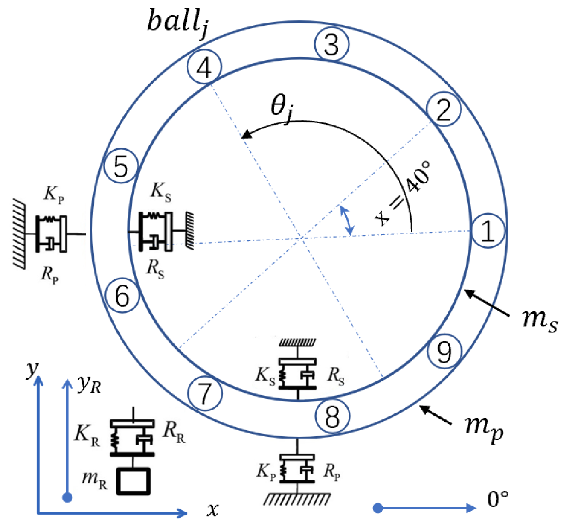
2.1. The Nonlinear 5-DoF Model
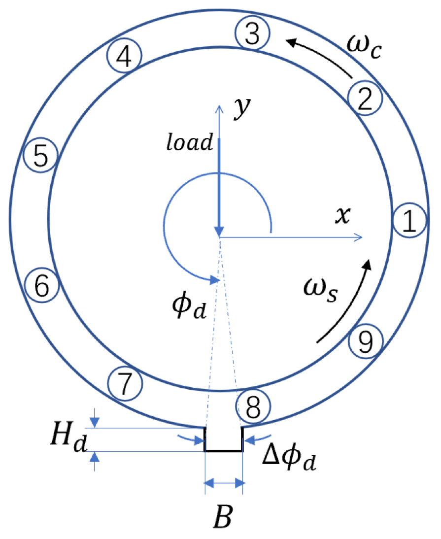
2.2. Bearing Defect Model
3. Model Implementation in Modelica and Model Calling in Python
3.1. Overview of the Virtual Bearing Test Bench in Modelica
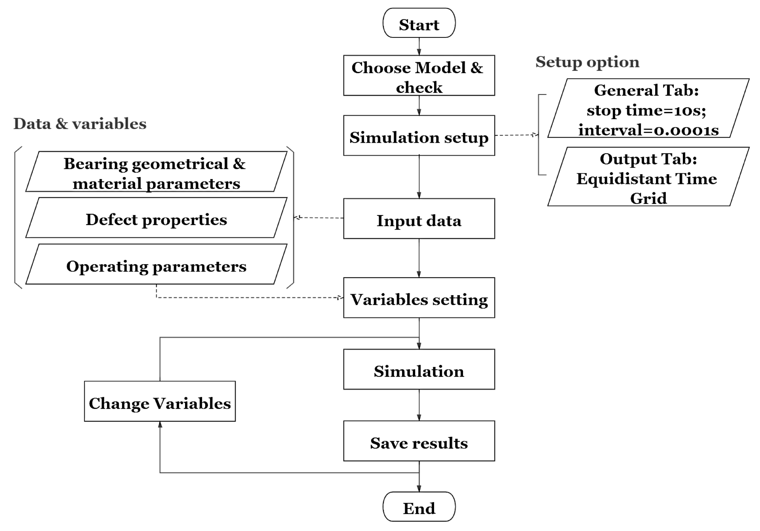
3.2. Procedure of Simulation with Virtual Bearing Test Bench in Modelica
3.3. Calling Modelica Model in Python with OMPython
3.4. Bearing Dynamics Model Validation
4. Bearing Fault Diagnosis Based on CNN
4.1. Cnn Structure and Hyperparameters
4.2. Feature Extraction from Time and Frequency Domains
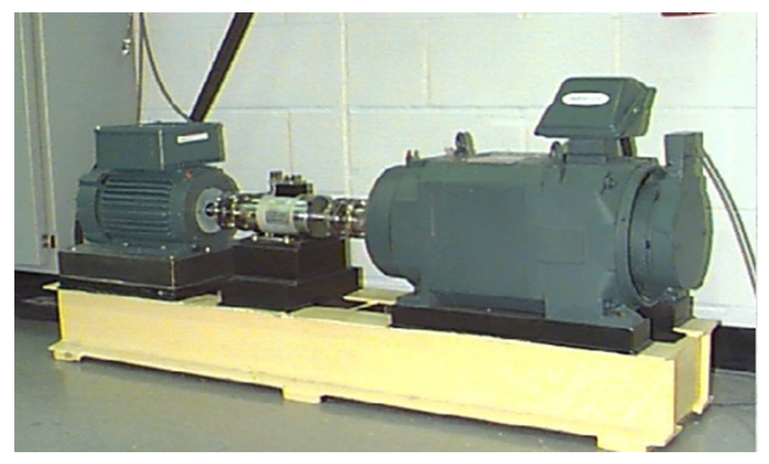
4.3. Experimental Set Up and Data Preprocessing
5. Direct Transfer Learning from Simulation Model to Bearing Test Bench
5.1. Procedure Overview of Direct Transfer Learning
5.2. Validation Case Design
5.3. Results of Direct Transfer Learning on Fault Diagnosis
5.3.1. Case A
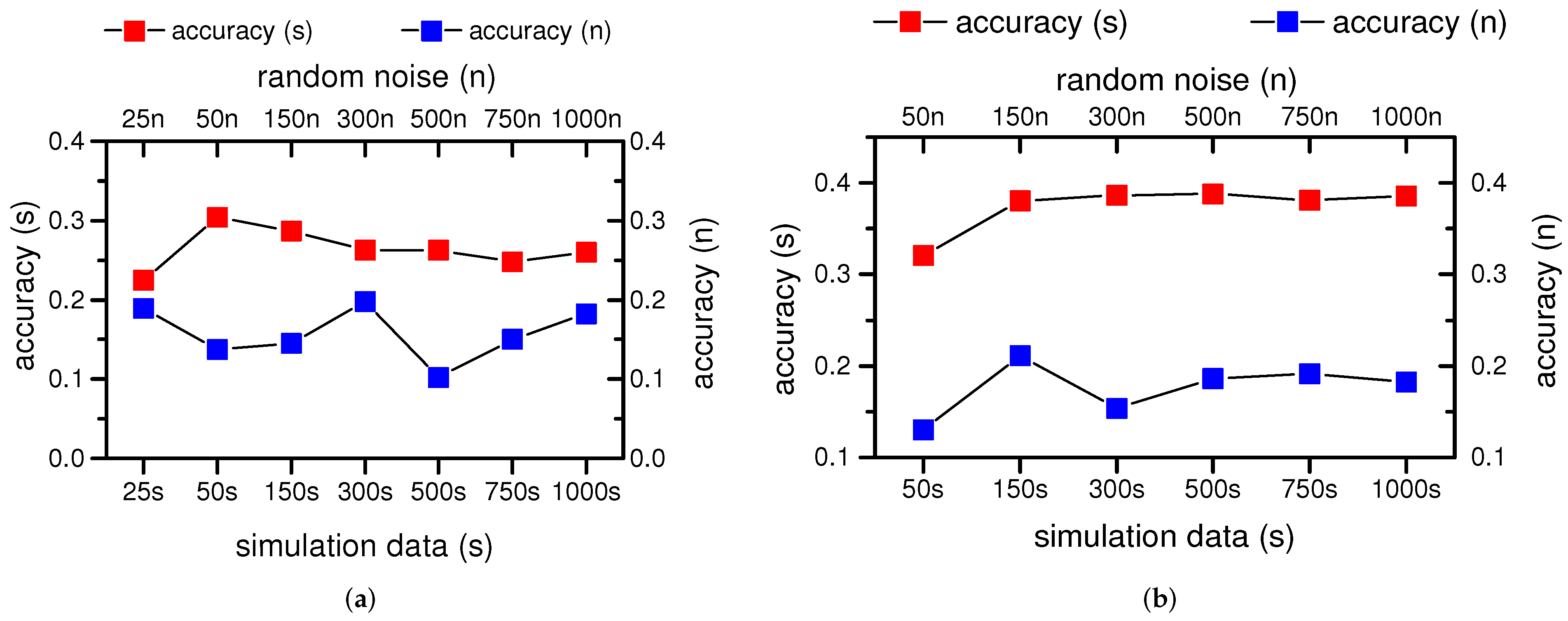
5.3.2. Case B
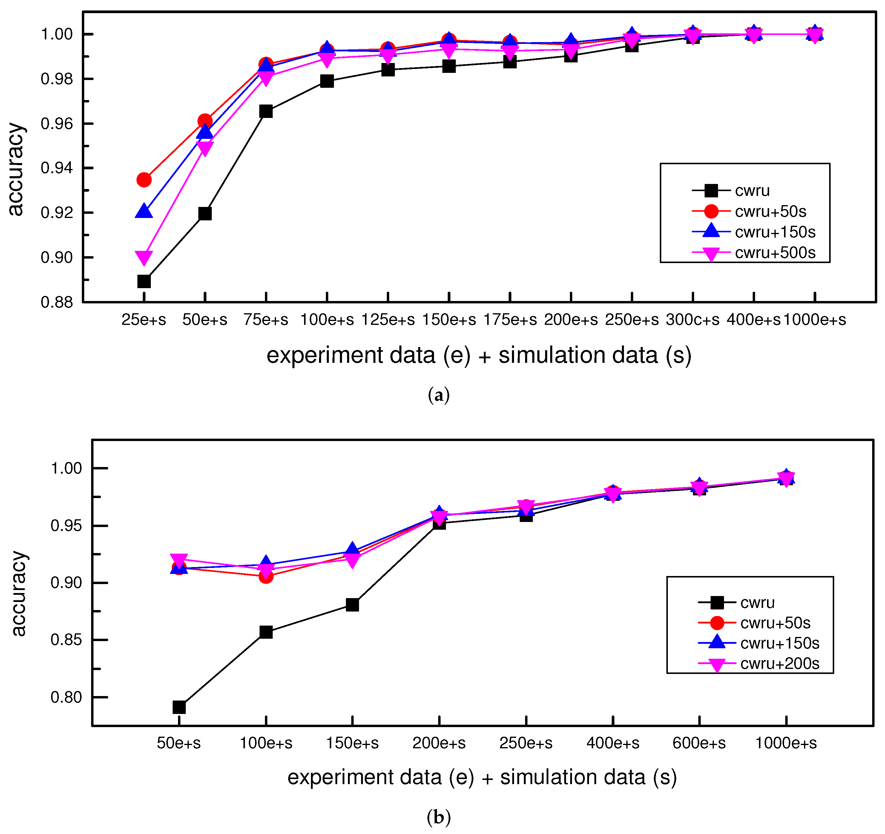
5.3.3. Case C
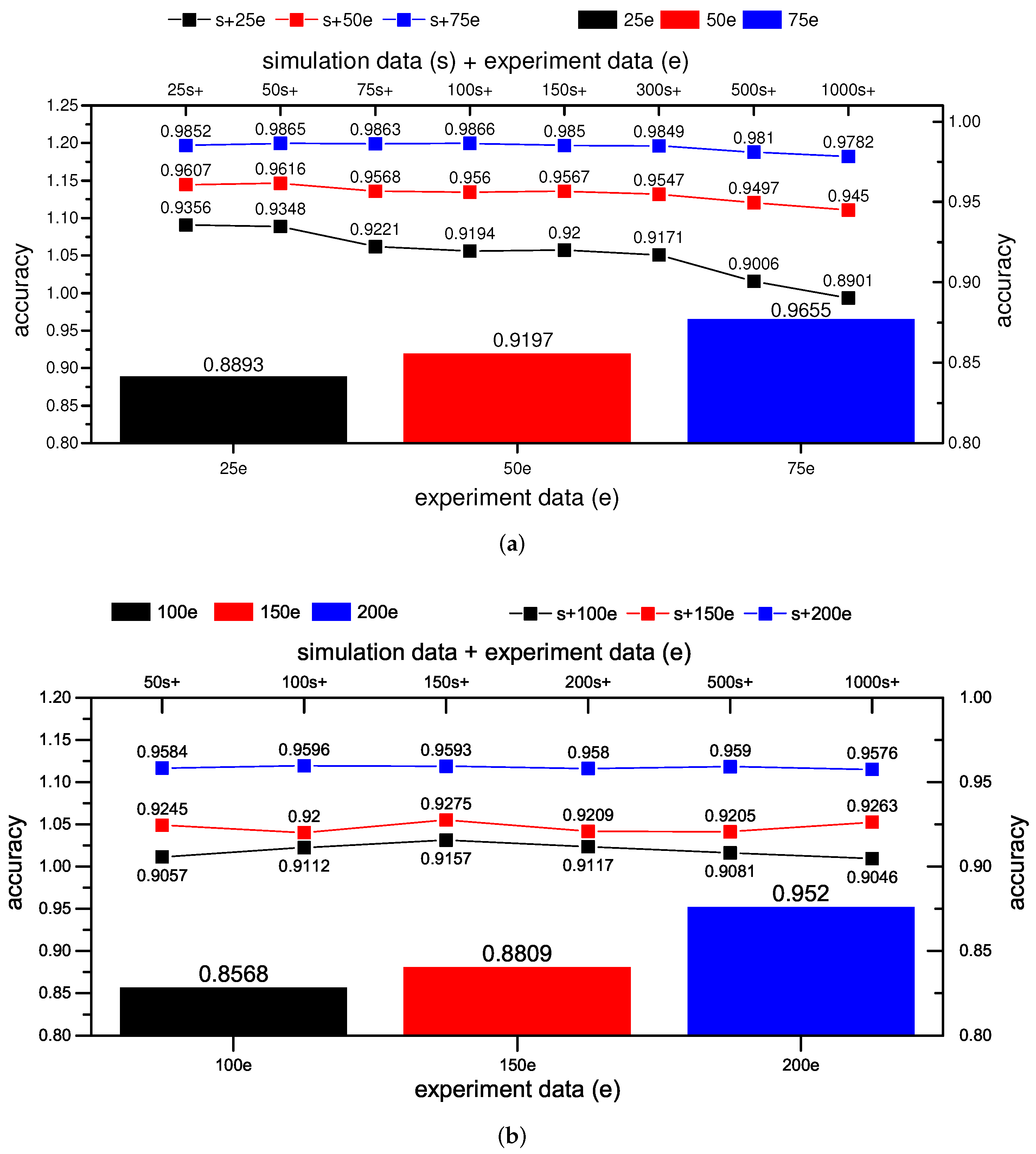
5.3.4. Case D
6. Conclusions
- A virtual bearing test bench has been developed in OpenModelica, with test bearing, driving motor, hydraulic loading and connecting shaft considered. As to the test bearing, besides normal dynamics modeling with the 5-DoF model, the modeling of fault position, shape and size, multiple faults are also addressed.
- The OpenModelica-based virtual bearing test bench is called in Python environment with OMPython and a developed GUI, which serves as a general study platform for data-driven bearing fault diagnosis.
- The simulation data generated from the dynamics model are used to train CNN after feature extraction. The trained-CNN is transferred directly to achieve fault diagnosis under the experimental dataset. Four different validation cases are designed to confirm the simulation data’s positive effect in the CNN’s direct transfer learning for bearing fault diagnosis.
Author Contributions
Funding
Data Availability Statement
Acknowledgments
Conflicts of Interest
Abbreviations
| PHM | Prognostics and Health Management |
| CNN | Convolutional Neural Networks |
| GAN | Generative Adversarial Network |
| DoF | Degree of Freedom |
| PSO | Particle Swarm Optimization |
| BPFO | Ball Passing Frequency on Outer race |
| BPFI | Ball Passing Frequency on Inner race |
| BSF | Ball Spin Frequency |
| CWRU | Case Western Reserve University |
| GUI | Graphical User Interface |
References
- Janssens, O.; Slavkovikj, V.; Vervisch, B.; Stockman, K.; Loccufier, M.; Verstockt, S.; Van de Walle, R.; Van Hoecke, S. Convolutional neural network based fault detection for rotating machinery. J. Sound Vib. 2016, 377, 331–345. [Google Scholar] [CrossRef]
- Eren, L.; Ince, T.; Kiranyaz, S. A generic intelligent bearing fault diagnosis system using compact adaptive 1D CNN classifier. J. Signal Process. Syst. 2019, 91, 179–189. [Google Scholar] [CrossRef]
- Zhang, W.; Peng, G.; Li, C. Bearings Fault Diagnosis Based on Convolutional Neural Networks with 2-D Representation of Vibration Signals as Input. MATEC Web of Conferences. EDP Sci. 2017, 95, 13001. Available online: https://www.matec-conferences.org/articles/matecconf/abs/2017/09/matecconf_icmme2017_13001/matecconf_icmme2017_13001.html (accessed on 29 January 2022).
- Guo, X.; Chen, L.; Shen, C. Hierarchical adaptive deep convolution neural network and its application to bearing fault diagnosis. Measurement 2016, 93, 490–502. [Google Scholar] [CrossRef]
- Wang, D.; Guo, Q.; Song, Y.; Gao, S.; Li, Y. Application of multiscale learning neural network based on CNN in bearing fault diagnosis. J. Signal Process. Syst. 2019, 91, 1205–1217. [Google Scholar] [CrossRef]
- Cordón, I.; García, S.; Fernández, A.; Herrera, F. Imbalance: Oversampling algorithms for imbalanced classification in R. Knowl.-Based Syst. 2018, 161, 329–341. [Google Scholar] [CrossRef]
- Ren, S.; Zhu, W.; Liao, B.; Li, Z.; Wang, P.; Li, K.; Chen, M.; Li, Z. Selection-based resampling ensemble algorithm for nonstationary imbalanced stream data learning. Knowl.-Based Syst. 2019, 163, 705–722. [Google Scholar] [CrossRef]
- Shao, S.; Wang, P.; Yan, R. Generative adversarial networks for data augmentation in machine fault diagnosis. Comput. Ind. 2019, 106, 85–93. [Google Scholar] [CrossRef]
- Zhang, W.; Li, X.; Jia, X.D.; Ma, H.; Luo, Z.; Li, X. Machinery fault diagnosis with imbalanced data using deep generative adversarial networks. Measurement 2020, 152, 107377. [Google Scholar] [CrossRef]
- Cui, L.; Chen, X.; Chen, S. Dynamics modeling and analysis of local fault of rolling element bearing. Adv. Mech. Eng. 2015, 7, 262351. [Google Scholar] [CrossRef] [Green Version]
- Liu, J.; Shao, Y.; Lim, T.C. Vibration analysis of ball bearings with a localized defect applying piecewise response function. Mech. Mach. Theory 2012, 56, 156–169. [Google Scholar] [CrossRef]
- McFadden, P.; Smith, J. The vibration produced by multiple point defects in a rolling element bearing. J. Sound Vib. 1985, 98, 263–273. [Google Scholar] [CrossRef]
- Ho, D.; Randall, R. Optimisation of bearing diagnostic techniques using simulated and actual bearing fault signals. Mech. Syst. Signal Process. 2000, 14, 763–788. [Google Scholar] [CrossRef]
- Cong, F.; Chen, J.; Dong, G.; Pecht, M. Vibration model of rolling element bearings in a rotor-bearing system for fault diagnosis. J. Sound Vib. 2013, 332, 2081–2097. [Google Scholar] [CrossRef]
- Ruan, D.; Li, Z.; Gühmann, C. Modeling of A Bearing Test Bench and Analysis of Defect Bearing Dynamics in Modelica. In Proceedings of the 14th International Modelica Conference, Linköping, Sweden, 20–24 September 2021; Sjölund, M., Buffoni, L., Pop, A., Ochel, L., Eds.; Number 181 in Linköping Electronic Conference Proceedings. Modelica Association and Linköping University Electronic Press: Linköping, Sweden, 2021; pp. 373–382. [Google Scholar] [CrossRef]
- Mishra, C.; Samantaray, A.; Chakraborty, G. Ball bearing defect models: A study of simulated and experimental fault signatures. J. Sound Vib. 2017, 400, 86–112. [Google Scholar] [CrossRef]
- Lie, B.; Bajrachary, S.; Mengist, A.; Buffoni, L.; Kumar, A.; Sjölund, M.; Asghar, A.; Pop, A.; Fritzson, P. API for accessing OpenModelica models from Python. In Proceedings of the 9th EUROSIM Congress on Modelling and Simulation, Oulu, Finland, 12–16 September 2016; pp. 707–714. [Google Scholar]
- Randall, R.B.; Antoni, J. Rolling element bearing diagnostics—A tutorial. Mech. Syst. Signal Process. 2011, 25, 485–520. [Google Scholar] [CrossRef]
- Ruan, D.; Zhang, F.; Gühmann, C. Exploration and Effect Analysis of Improvement in Convolution Neural Network for Bearing Fault Diagnosis. In Proceedings of the 2021 IEEE International Conference on Prognostics and Health Management (ICPHM), Detroit, MI, USA, 7–9 June 2021; pp. 1–8. [Google Scholar]
- Saruhan, H.; Saridemir, S.; Qicek, A.; Uygur, I. Vibration analysis of rolling element bearings defects. J. Appl. Res. Technol. 2014, 12, 384–395. [Google Scholar] [CrossRef]
- Lei, Y.; Yang, B.; Jiang, X.; Jia, F.; Li, N.; Nandi, A.K. Applications of machine learning to machine fault diagnosis: A review and roadmap. Mech. Syst. Signal Process. 2020, 138, 106587. [Google Scholar] [CrossRef]
- Chen, C.; Li, Z.; Yang, J.; Liang, B. A cross domain feature extraction method based on transfer component analysis for rolling bearing fault diagnosis. In Proceedings of the 2017 29th Chinese Control and Decision Conference (CCDC), Chongqing, China, 28–30 May 2017; pp. 5622–5626. [Google Scholar]
- Tong, Z.; Li, W.; Zhang, B.; Jiang, F.; Zhou, G. Bearing fault diagnosis under variable working conditions based on domain adaptation using feature transfer learning. IEEE Access 2018, 6, 76187–76197. [Google Scholar] [CrossRef]
- Li, X.; Zhang, W.; Ding, Q. Cross-domain fault diagnosis of rolling element bearings using deep generative neural networks. IEEE Trans. Ind. Electron. 2018, 66, 5525–5534. [Google Scholar] [CrossRef]
- Han, T.; Liu, C.; Yang, W.; Jiang, D. A novel adversarial learning framework in deep convolutional neural network for intelligent diagnosis of mechanical faults. Knowl.-Based Syst. 2019, 165, 474–487. [Google Scholar] [CrossRef]
- Shen, F.; Chen, C.; Yan, R.; Gao, R.X. Bearing fault diagnosis based on SVD feature extraction and transfer learning classification. In Proceedings of the 2015 Prognostics and System Health Management Conference (PHM), Beijing, China, 21–23 October 2015; pp. 1–6. [Google Scholar]
- Zhang, R.; Tao, H.; Wu, L.; Guan, Y. Transfer learning with neural networks for bearing fault diagnosis in changing working conditions. IEEE Access 2017, 5, 14347–14357. [Google Scholar] [CrossRef]


| Hyperparameter | Value |
|---|---|
| Drop rate | 0.55 |
| Learning rate | 0.0006 |
| Kernel size of the 1st layer | 5 × 5 |
| Kernel size of the 2nd layer | 3 × 3 |
| Number of filters in the 1st layer | 128 |
| Number of filters in the 2nd layer | 256 |
| Batch size | 110 |
| Density layer (flatten) | 512 |
| Number | Feature |
|---|---|
| 1 | Mean |
| 2 | Standard deviation |
| 3 | Skewness |
| 4 | Kurtosis |
| 5 | Max |
| 6 | Min |
| 7 | Range |
| 8 | Median |
| 9 | Variance |
| 10 | Root mean square |
| 11 | Impulse factor |
| 12 | Crest factor |
| 13 | Shape factor |
| Number | Feature | Number | Feature |
|---|---|---|---|
| 14–21 | 1st BPFI | 110–117 | 5th BPFOI |
| 22–29 | 1st BPFO | 118–125 | 5th BPFO |
| 30–37 | 1st BSF | 126–133 | 5th BSF |
| 38–45 | 2nd BPFI | 134–141 | 6th BPFI |
| 46–53 | 2nd BPFO | 142–149 | 6th BPFO |
| 54–61 | 2nd BSF | 150–157 | 6th BSF |
| 62–69 | 3rd BPFI | ||
| 70–77 | 3rd BPFO | ||
| 78–85 | 3rd BSF | ||
| 86–93 | 4th BPFI | ||
| 94–101 | 4th BPFO | ||
| 102–109 | 4th BSF |
| Fault Type | Fault Diameter (unit: inches) | Sample Size of Training Set | Sample Size of Test Set | Labels |
|---|---|---|---|---|
| Ball failure | 0.021 | 197 | 197 | 1 |
| Inner race failure | 0.021 | 197 | 197 | 2 |
| Outer race failure | 0.021 | 197 | 197 | 3 |
| Health | 0.021 | 409 | 409 | 0 |
| Sum | / | 1000 | 1000 | / |
| Case | 0.014/0.021 inches | |
|---|---|---|
| Train Set | Test Set | |
| Case A | Exp. data (increasing) | Exp data (1000 sets) |
| Case B | Sim. data (increasing) | |
| Case C | Exp. data (increasing) + Sim. data (fixed) | |
| Case D | Exp. data (fixed) + Sim. data (increasing) | |
Publisher’s Note: MDPI stays neutral with regard to jurisdictional claims in published maps and institutional affiliations. |
© 2022 by the authors. Licensee MDPI, Basel, Switzerland. This article is an open access article distributed under the terms and conditions of the Creative Commons Attribution (CC BY) license (https://creativecommons.org/licenses/by/4.0/).
Share and Cite
Ruan, D.; Chen, Y.; Gühmann, C.; Yan, J.; Li, Z. Dynamics Modeling of Bearing with Defect in Modelica and Application in Direct Transfer Learning from Simulation to Test Bench for Bearing Fault Diagnosis. Electronics 2022, 11, 622. https://doi.org/10.3390/electronics11040622
Ruan D, Chen Y, Gühmann C, Yan J, Li Z. Dynamics Modeling of Bearing with Defect in Modelica and Application in Direct Transfer Learning from Simulation to Test Bench for Bearing Fault Diagnosis. Electronics. 2022; 11(4):622. https://doi.org/10.3390/electronics11040622
Chicago/Turabian StyleRuan, Diwang, Yuxiang Chen, Clemens Gühmann, Jianping Yan, and Zhirou Li. 2022. "Dynamics Modeling of Bearing with Defect in Modelica and Application in Direct Transfer Learning from Simulation to Test Bench for Bearing Fault Diagnosis" Electronics 11, no. 4: 622. https://doi.org/10.3390/electronics11040622
APA StyleRuan, D., Chen, Y., Gühmann, C., Yan, J., & Li, Z. (2022). Dynamics Modeling of Bearing with Defect in Modelica and Application in Direct Transfer Learning from Simulation to Test Bench for Bearing Fault Diagnosis. Electronics, 11(4), 622. https://doi.org/10.3390/electronics11040622