Electricity Consumption Prediction in an Electronic System Using Artificial Neural Networks

Abstract

The tremendous rise of electrical energy demand worldwide has led to many problems related to efficient use of electrical energy, consequently posing difficult challenges to electricity consumers of all levels—from households to large companies’ facilities. Most of these challenges could be overcome by the accurate prediction of electricity demand. Additionally, balance responsibility includes the penalty-based financial mechanism causing extra expense for badly estimated consumption, above the allowed imbalance limits. In this paper, a method for electricity consumption prediction based on artificial neural networks is proposed. The electricity consumption dataset is obtained from a cold storage facility, which generates data in hourly intervals. The data obtained are measured for a period of over 2 years and then separated to four seasons, so different models are developed for each season. Five different network structures (ordinary RNN, LSTM, GRU, bidirectional LSTM, bidirectional GRU) for five different values of horizon, i.e., input data (one day, two days, four days, one week, two weeks) are examined. Performance indices, such as mean absolute percentage error (MAPE), root mean square error (RMSE), mean absolute error (MAE) and mean square error (MSE), are used in order to obtain qualitative and quantitative comparisons among the obtained models. The results show that the modifications of recurrent neural networks perform much better than ordinary recurrent neural networks. GRU and LSTMB structures with horizons of 168h and 336h are found to have the best performances.

1. Introduction

In the last two decades, the liberalization of the electric power sector has affected much in all industries, leading to very dynamic wholesale markets, where traders are focused on price dynamics trends. On the other hand, retail markets are fairly deregulated, so in the phase of supplying electricity to final consumers, the prediction of consumption can play a great role in fostering cost-efficiency [1]. Industry efficiency investment is heavily affected by the enabling efficiency policies, such as energy performance standards and incentive mechanisms for energy savings and emissions reductions [2].

The prediction of energy consumption is possible in the short-term, mid-term and long-term. Which of these is used depends on many factors but all of them can be essential in the phase of defining strategies for production planning and the expansion of infrastructure capacities for electric power systems. Tools for strategic planning are more certain and precise when proper models for determining the patterns of individual consumers are available. In that case, the consumption prediction of each individual consumer can be valuable on the aggregated level. In this paper, we performed short-term forecasting.

An overview of short-term electrical load forecasting (STLF) methodologies, which included different linear and non-linear parametric methodologies, was given in [3]. In that paper, the electrical load data and meteorological data of one city in Pakistan were used in order to obtain the most efficient model that predicts the electrical load. Based on extensive research presented in the paper, the most accurate model is proposed. One more example where STLF was proven to be valuable for electrical load prediction and scheduling in power systems was given in [4], where a novel two-stage encoder–decoder was used. A hybrid model was proposed, integrating convolutional neural networks and bidirectional LSTM. However, both short- and medium-term electrical load forecasting were presented in [5] using a genetic algorithm-based non-linear auto-regressive neural network model.

Balance responsibility [6] refers to the penalty-based financial mechanism developed to force market participants to properly anticipate their energy needs on a short-term basis. This mechanism functions in a way that electric power suppliers inform transmission system operator (TSO) as to what amount of electric power is to be provided on hourly level for all his consumers for the day ahead. This information is of crucial importance, because the TSO needs to maintain a real-time balance between production and consumption for the entire system, based on the data, which are gathered from all active balancing parties. Of course, there is always a certain tolerance given to balancing parties. However, if predicted consumptions do not match actual consumed energy and the tolerance for imbalance is above certain limits, the balancing party is penalized. These penalty prices are defined for each hour retroactively, based on pre-established methodology issued by the regulatory body, so the responsible market participant pays for each hour proportionally to the imbalance created in the system. That means that if the electric power supplier does not have an adequate forecasting tool and gives poor forecasting regarding how much electricity is needed in each hour in its balancing group, extra expense occurs for each bad estimation above the allowed imbalance limits for measured consumption. Electricity balancing market design is quite a challenge [7], and balancing responsibility is one of the variables that need to be planned in this process. Balancing responsibility is presented for different countries and markets in executive summaries of TSOs, within ENTSO-E Balancing report 2022 [8]. In liberalized power markets, balance responsibility and imbalance settlements are two closely related elements constituting the essential part of a balancing market [6].

The importance of electricity consumption prediction on one hand and its complexity on the other hand has motivated many researchers in this area. In the literature, there are numerous studies on electricity consumption and demand estimation. Electricity demand is heading for its fastest growth in more than 10 years. Global energy demand is set to increase by 4.6% in 2021, surpassing pre-COVID-19 levels [9]. In these studies, research on electrical energy consumption forecasting has evolved into many methods that can be roughly categorized [10] into artificial intelligence (AI)-based methods [11,12] and conventional methods [13,14,15]. Conventional models most commonly use ARMA models (autoregressive–moving-average models), such as in [13] for modeling electricity loads or ARIMA models (autoregressive integrated moving average models) in [14] for energy consumption forecasting. Additionally, some of the commonly used methods are stationary time series models [16], regression models [17,18,19] and econometric models [20]. In [21], a review of all these techniques is given and implemented to electric energy forecasting in Chile.

However, most of time series models are linear predictors, while electricity consumption is an inherently a nonlinear function. So, the behavior of electricity consumption series may not be completely captured by the time series techniques. To solve this problem, other research papers have proposed Artificial Neural Networks (ANN) and genetic algorithms for electricity consumption forecasting [22,23].

The main purpose of the study presented in this paper is to develop adequate seasonal model for predicting electricity consumption for an individual electronic system using measured hourly-based consumption data. These models are then supposed to be used to properly estimate energy needs on an hourly level, meaning that they can be an appropriate tool for the electric power supplier to avoid unnecessary imbalance costs. After modeling, the evaluation is performed to estimate the accuracy of the forecasting model using key performance indicators, such as mean absolute percentage error (MAPE), root mean square error (RMSE), mean absolute error (MAE), mean square error (MSE). The results show that the GRU and LSTMB structures with horizons of 168 h and 336 h perform the best.

For the purpose of this study, United Green Energy Ltd. [24], a consulting company for the energy market from Serbia, has provided data of an individual consumer, a cold storage facility in this specific case. Data were strategically chosen so irregular intermittent consumption profile was able to be used as the input data set. Autocorrelation analysis is implemented in order to select the inputs to different network structures. The proposed methodology is only presented using this specific example, but it can be applied to different electronic systems that consume energy.

Considering the above-stated, the main contributions of this research paper are as follows:

• Seasonal models are developed to predict amount of consumed energy based on measured hourly-based consumption data provided for this purpose from a cold storage facility in Serbia;
• Data analysis is performed in order to select the inputs to different network structures;
• Several performance indicators are used to estimate performances of the proposed models. Based on these criteria, the best models are chosen.

2. Data and Methods

In order to solve prediction problems, a quantity is usually represented as a time series and then the values from a number of consecutive time steps in series are taken as an input to a mathematical model, which generates predicted value(s) for the next timestep(s). Traditionally, mathematical models used on forecasting time series employ statistical methods, such as ARIMA, exponential smoothing, etc., but using these methods requires some of the statistical properties of data to be predicted and to fulfil some conditions, i.e., the data must be stationary in order to gain reasonable prediction results. Recently, deep learning models [25,26] have been recognized as an important tool for solving prediction problems due to the simplicity of implementation and availability of software, which allows neural network models to be easily created and machine learning algorithms to be flexibly implemented. Another reason is that unlike statistical models, neural networks can perform well even without examining the statistical properties of data.

Along with statistical methods, various machine learning algorithms have been extensively used for time series prediction and have shown good results in performing such tasks [27]. ML algorithms are also known to be able to perform well on larger datasets when compared to statistical methods [28]. Examples of such algorithms include:

K-nearest neighbor (k-NN)—based on a given set of input–output vector pairs, a prediction for each new input query is made considering the outputs of K most similar input vectors in the set. Most commonly used metrics for representing the similarity between two vectors are the Euclidean distance, the Manhattan distance or the Minkowski distance, which is a generalized version of the previous two [29]. The outputs of K vectors with the smallest distance from the input query can be averaged or interpolated to create a new prediction [30]. The advantages of this algorithm is its simplicity, the absence of training period and that it only depends on one parameter, but some of its flaws are that the calculations and sorting of distances must be performed every time a new input is presented and that it is very sensitive to outliers [31].

Support vector machine (SVM) regression—in this algorithm, the predictor function is optimized in such a way that none of its values differ from any of the outputs from the test set by a predefined parameter ε and so that it is as linear as possible [32]. Advantages of this method are high accuracy, a good generalization of test data and computational complexity being independent of the input data dimension [33].

Random forest—random forest models are based on a technique commonly known as bagging (bootstrapping and aggregation). The model consists of multiple decision trees where each tree is trained on a distinct subset of the training set called the bootstrap set. Outputs at the leaves of each tree are averaged (aggregated) to produce the prediction for the corresponding input. The key advantage is its structure, as multiple decision trees trained on different data have shown to give better accuracy and are less prone to overfitting [34].

The most popular type of neural network models used in time series prediction problems [35] is the recurrent neural network (RNN) structure [36]. Unlike traditional feed-forward networks where the weights, connecting hidden layers, are directed from the input to the output, RNNs introduce temporal feedback connections in such way that the outputs of an RNN depend not only on the current input data but also on the data presented to the network in previous timesteps. In this way, RNNs are capable of capturing temporal dependence and patterns within data, which makes them suitable for time series prediction.

As a concept, RNNs originated in the 1980s and have undergone numerous improvements in terms of performance and complexity since then. Many new versions of RNN structures have emerged lately, most popular of which are long short-term memory (LSTM) [37] and gated recurrent unit (GRU) [38]. These models have found their use in many fields of science and technology ranging from internet search engines to speech recognition.

In this paper, the structure of the LSTM and GRU models, but also of bidirectional LSTM and GRU, are discussed and applied to solve the problem of electricity consumption prediction, comparing their capabilities with classical RNN structures. At the end, the model of the best network structure is presented.

Electrical consumption is often influenced by different climatic factors, such as temperature and humidity [2]. Therefore, the short-term prediction models often include meteorological and temporal parameters [5], [39], temperature and wind speed [40], humidity and total precipitable liquid water [41]. Additionally, there is a distinction between working days and weekends or holidays because they show different electrical load-consuming profiles. This feature is taken into account in [42] where “Working Day feature” is a parameter. In the work presented in this paper, meteorological data are not used as network inputs but only amount of consumed energy. This led us to research what is an adequate prediction horizon and whether these data are enough for good prediction. Obtained results will be discussed in subsequent sections.

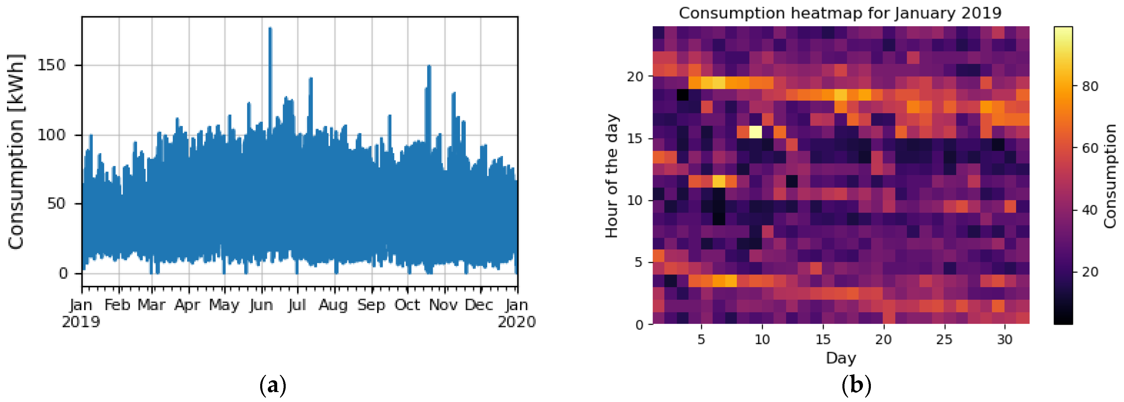
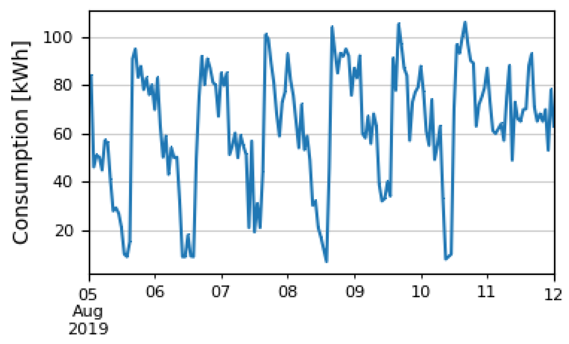
2.1. Consumption Dataset

The electricity consumption dataset is obtained from a cold storage facility, which uses a consumption measurement system that generates data in hourly intervals. The data obtained are measured in kWh (kilowatt-hour), and measurements are taken for the period from 1 January 2019 to 28 February 2021, containing a total of 18,960 data points for a period of over 2 years. Figure 1a presents the raw values of consumption recorded during the year 2019. Measured consumption values are quantized with a quantization step of 0.128 kWh. In Figure 1b, we present the consumption heatmap for January 2019. From the figure it is obvious that consumption is lowest at noon and highest during the early evening.

It is expected for such types of data to indicate seasonality. By exploring the dataset in more detail, we can see that the consumption values change periodically, i.e., the consumption time series shows a seasonal pattern. An example of this pattern for one week is shown in Figure 2.

First, it is obvious that the consumption is higher in the period between midnight and early morning hours (60–110 kWh), then it drops to its lowest level around noon and then reaches peak value in the early afternoon. After that, it is again in the 60–110 kWh range in the afternoon. Such behavior is typical for every day during the week, except on Sunday, when there is no drop around noon. This obvious week seasonality is very well captured, so it is expected that the neural network model could easily find this pattern.

The electricity consumption dataset is separated into four seasons: December, January and February comprise the winter season; March, April and May comprise the spring season; June, July and August comprise the summer season; and September, October and November comprise the autumn season. A separate model is developed for each season. The winter dataset is the biggest, since in our measured set there are data for three Januaries and three Februaries (2019, 2020, 2021), and for other months we have data for 2 years (2019, 2020).

The width of the input horizon is determined by autocorrelation coefficient analysis. Autocorrelation function shows to what extent a time series is in correlation with its copy shifted in time by a number of time intervals (lags). Autocorrelation coefficients are values between −1 and 1, which show the amount of autocorrelation for a given lag. Values close to 1 or −1 show that there is a strong positive/negative autocorrelation, while values close to 0 show that the autocorrelation is weak. Figure 3 shows the autocorrelation plot for the consumption time series over 168 lags, which corresponds to a period of one week. From the plot, it can be seen that the correlation is very strong between each two consecutive time steps and that it reaches its peaks at lags that are multiples of 24. Autocorrelation peaks are lower for lags which correspond to periods of about four days (96 h) but are somewhat larger for a lag of one week. Considering this information, input data horizons are chosen to be multiples of 24, more precisely: 24, 48, 96, 168 and 336.

2.2. Anomalies in Dataset

It can be seen from the Figure 1a that there are values that jump out from the others, i.e., slight anomalies occur. Consumption usually ranges from 5 to 120 kWh, but at some points it reaches values of over 150 kWh. The cause of the appearance of such minor anomalies could be the malfunctioning of devices that in some rare cases consume more energy than usual, the malfunctioning of the system for measuring consumption or the improper entry of data. Therefore, there are several possible causes of anomalies where some of them may be unpredictable events. In addition to these anomalies, it also happens that for some dates consumption values are not given at all but that space in the data is filled with zeros.

Any kind of larger anomaly will negatively affect the prediction accuracy of the neural network. With the appearance of the wrong data or lack of data, the network stops learning the correct patterns and learns new ones, in which zero or excessive values appear in many places. Such problems are often solved by replacing absurd or non-existent values with new estimated values that are determined to fit the properties of the time series being analyzed, i.e., the new value should not disturb the trend and seasonality (if any) or the values of the autocorrelation coefficients. Smaller anomalies do not need usually to be discarded, since there is a chance that they were not caused by incorrect data entries but due to some other circumstances, and their influence on the accuracy of the prediction is much smaller. There are various methods for inserting valid values into a time series that vary in complexity and the shape of the time series or the data in general. Depending on the used method, the estimation of the new values can be rougher or more accurate.

Anomalies can be seen as values that appear infrequently in a data set and deviate significantly from the average. They are most easily removed by setting some upper and lower bounds and in this way any elements that do not fall within that range are deleted from the array. It is clear that anomalies can be detected visually. From the graph, the places where the time series takes values that are not valid can be seen. Moreover, from the graph it is not possible to clearly read the range moves of these values. For example, by searching for a set of consumption data, one can come to the conclusion that its value rarely exceeds 110 kWh, so that value can be set as a limit.

Another procedure for detecting anomalies that is often used in statistics is the calculation of the zscore, i.e., the z-value, which is based on the standard deviation. To remove anomalies, it is enough to calculate the zscore for each datum and if a value outside this range is obtained, the data are considered an anomaly and can be deleted from the set.

Additionally, there are various methods for inserting valid data where consumption values are not given at all. Some of them are very simple to implement, but they give very rough estimates. Other methods are more complex but give more than satisfactory results. For missing data in this research an interpolation technique is applied.

2.3. Preparation of Data for Training and Testing

Since the dataset is repaired before starting the training process, it is necessary to adapt the dataset to the implementation of the neural network model. As previously stated, a many-to-one configuration is used with the number of inputs equal to the prediction horizon (h), and one output. Therefore, for each prediction, a vector of h data representing the input sequence of consecutive observations is provided. The output is expected to be the estimated value of the next observation in the sequence. Data are organized into input–output pairs (X-Y) according to the so-called sliding window technique, as shown in the

Table 1. Preparation of the dataset.

No.	i	X							Y
		xi−h+1	xi−h+2	xi−h+3	xi−h+4	xi−h+5	…	xi	xi+1
1	h	36.992	52.096	48	23.936	49.024	…	64	17.024
2	h + 1	52.096	48	23.936	49.024	64	…	20.992	23.936
3	h + 2	48	23.936	49.024	64	20.992	…	29.952	32
4	h + 3	23.936	49.024	64	20.992	29.952	…	24.064	25.984
5	h + 4	49.024	64	20.992	29.952	24.064	…	29.952	12.032
…	…	…	…	…	…	…	…	…	…
n − h + 1	n	38.912	26.112	38.912	35.072	51.968	…	36.096	43.008

.

A total of n − h + 1 input–output pairs is created from the time series of total n input data. The first pair contains the input vector of observations indexed in the series from 1 to h and the expected output is the observation at time h + 1. The second pair contains observations from 2 to h + 1, and the output is an observation at time h + 2, etc. The input and output vectors organized in this way are further divided into a training and a test set. A certain percentage (usually 30%) of the total n − h + 1 data is taken and saved for testing the network, and the rest is used for training. Finally, it should be noted that all data from the series are scaled so that their values fall into the range between 0 and 1. It is important the data to be in the smallest possible range since LSTM and GRU structures have a larger number of units that work with sigmoid and tanh functions.

3. Choosing an Optimal ANN Structure

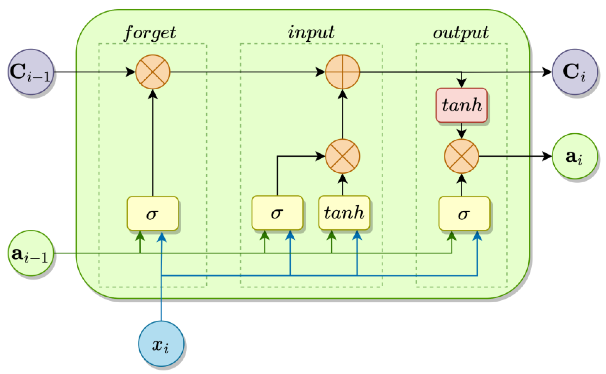
Neural networks consist of several layers of connected neurons and are characterized by different architectures, which predetermine certain properties [43,44]. In processing, data are propagated through the network, moving from input to output via connections between neurons. The way neurons are connected has a significant impact on the result of data processing. According to the flow of data through the layers of the neural network, two types of networks are distinguished—feedforward, i.e., with forward propagation (FF), and recurrent (Recurrent Neural Network—RNN).

The FF structure is simple to implement and generally has good performance, so it is very often encountered in solving various machine learning problems, such as linear regression and classification problems. However, this structure does not provide a good basis for problems in which it is necessary to analyze series of data, where the influence of previously entered data on the output of the network as well as the sequence of appearance of data at the input is of key importance, so it cannot be expected that the FF structure will give good results when predicting time series. The reason for this is that when new data appears at the input, all activations within the network receive completely new values, which means that all information regarding the previously entered data are lost. In other words, the FF structure has no memory.

The main difference between FF and RNN structures is that recurrent neural networks contain feedback connections between neurons, so introducing RNN solves the memory problems [45,46].

A neural network is recurrent if there are connections within it that the bind neurons of one layer with neurons from the previous layer or with neurons within the same layer. Activations generated in neurons by the current input are stored in the neuron until the next input is ready. Then, activations are transmitted via feedback loops to neurons from previous layers, where they arrive together with new inputs and activations.

In this way, a memory effect is achieved, since information generated at previous inputs is to some extent retained and circulated through the network, having an impact on the output of the network. Due to such connections, the activation of one neuron does not only depend on the input of the network or the activation of the neurons from the previous layer but also on the activations generated by the same neuron at the previously supplied inputs of the network. Thus, the order of getting the input data has an effect on the output of the network—an input at one time can affect the output even after specifying a number of new inputs after it. Then, the network can establish regularities between the multiple consecutive members of a series fed to its input, which is suitable for predicting time series, especially if there is a strong correlation between series members several time points apart.

For the purposes of the time series analysis of consumption, the many to one configuration is suitable (Figure 4), because a sequence of observations in the length of one horizon can be led to the inputs, while the expected value of the first next observation is obtained at the output. For example, if the data are taken every hour and the forecast horizon is 12 h, then for the input data representing the consumption during one day between 9:00 a.m. and 8:00 p.m., the output represents the consumption estimate at 9:00 p.m. on the same day. After that, the predicted value is compared with the actual value in order to estimate the error, the actual value is added to the sequence of observations, and the oldest value is deleted. This moves the horizon forward one hour. Based on data taken between 10:00 a.m. and 9:00 p.m., the consumption at 10:00 p.m. is predicted and the whole process is repeated for each new observation.

3.1. LSTM Structure

LSTM [47] represents an advanced modification of the RNN unit that was created with the idea of solving the problem of vanishing gradients, and today this architecture is widely used for solving a wide variety of problems [48,49,50]. In addition to the standard recurrent neuron layer of the RNN unit, LSTM has four more neuron layers and each of them has a special function. Additionally, as well as containing the internal state that is transferred from unit to unit, in LSTM there is another channel that spans the data string and represents the main part of the LSTM unit. It is called the common state or cell state, marked with C_i in Figure 5. The cell state serves as long-term shared memory for multiple concurrent LSTM units and is used to store and update general information relevant to multiple units in the chain. Different units can add new or delete old information from the cell state, regardless of their distance from each other. The cell state is modified by applying several different activation functions to the inputs of the unit and the activation from the previous unit, and also according to the previous values that the cell state had. Neuron layers are arranged in a specific structure, which modifies the cell state so that the LSTM is resistant to the problem of vanishing gradients, which makes it very useful for applications where longer sequences need to be analyzed.

The update of the cell state is carried out through three blocks consisting of layers of neurons and their inputs are supplied with the current input and the internal state of the previous unit:

(1)

The forget gate is formed from a layer of neurons with a sigmoid activation function, so the activations of these neurons can have values between 0 and 1. The activations of the neurons are multiplied by the corresponding data in the array of cell states. If the activation is approximately 0, then the corresponding data from the cell state will be deleted, and if it is approximately 1, then the data will be kept.

(2)

The input gate examines whether some new information can be obtained from the current input and then whether this information is important for the state of the cells, i.e., if it should be added or ignored. The input gate consists of one sigmoid layer and one layer, activation function of which is the hyperbolic tangent. The hyperbolic tangent layer generates the information, and the σ layer decides which parts of the information should be passed to the cell state.

(3)

The output gate generates the output of the unit as well as the new internal state using the modified cell state. It consists of a σ layer that is applied to the input and the previous internal state and a layer, the activation of which is chosen as needed, generating the output data.

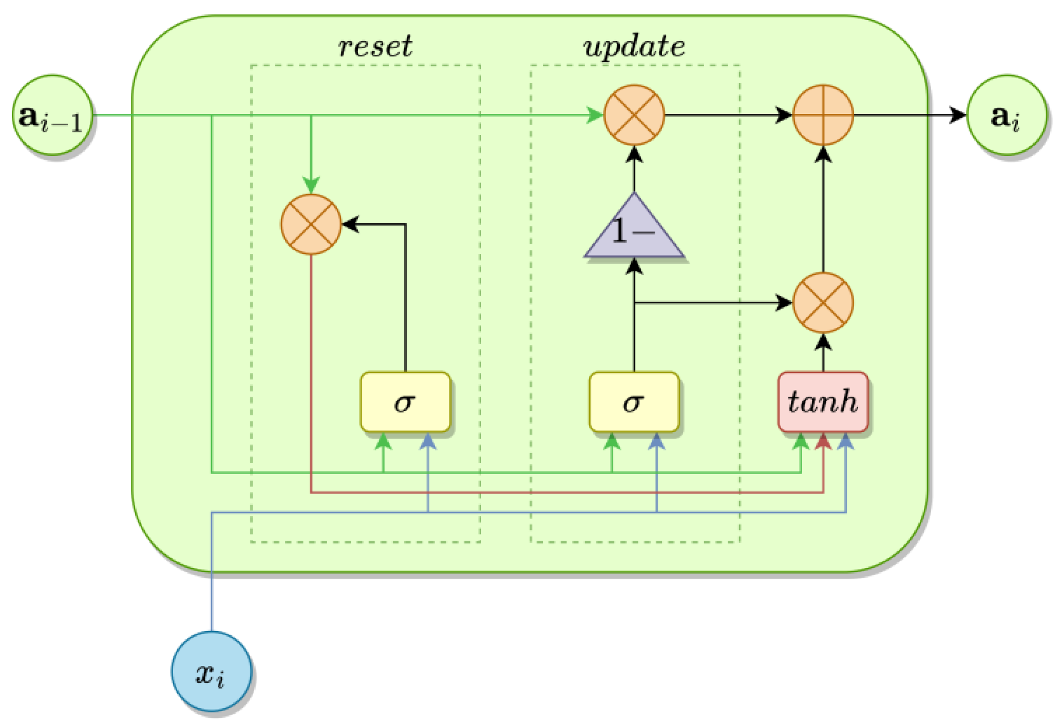
The LSTM structure has been shown to give very good results in solving sequence prediction problems and today is considered the most popular type of recurrent neural network. However, compared to a simple RNN structure, LSTM has a much larger number of neurons—approximately five times more neurons than in an RNN network of the same length. The number of weights is much higher than that, and networks with too many weights are memory intensive and in the case of a large input string length, memory overload may occur.

3.2. GRU Structure

There are various modifications of the LSTM structure that reduce the complexity of the network by removing or modifying individual blocks. One such configuration is the gated recurrent unit—GRU [51]. This configuration, shown on Figure 6, treats the previous internal states as a common state, so it contains only one channel for information transfer. Additionally, it consists of only two blocks—the reset block, which decides how much information from the previous state should be deleted, and the update block, which decides which information should be kept.

A smaller number of blocks and channels of information results in a smaller number of connections and therefore smaller memory requirements.

Table 2. Number of neurons for different configurations.

Network Configuration	Number of Neurons
RNN	n2 + 2n
LSTM	4·(n2 + 2n)
GRU	3·(n2 + 2n)

shows a comparison of different configurations according to the number of weight connections in hidden layers (including connections with activation thresholds), where it is assumed that all layers have the same number of neurons and that the input layer receives only one datum.

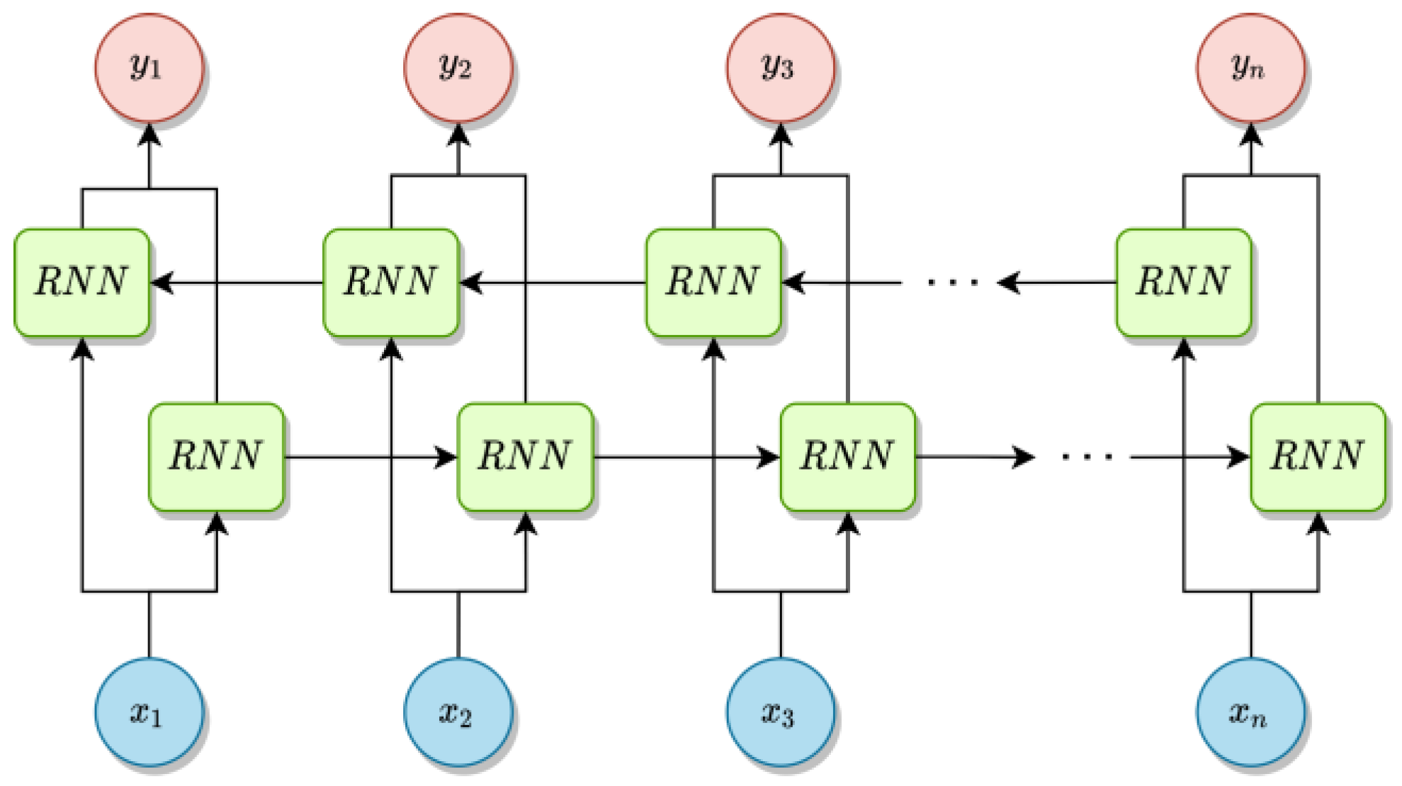
3.3. Bidirectional Recurrent Networks

Sometimes it is important to look at the input sequence in reverse chronological order. In this way, there is an opportunity for the network to learn new regularities and patterns according to which the observations change. This means practically that one should train the network with two sets of data—one consisting of the sequences in the correct order and one with the sequences reversed. Instead, a bidirectional configuration of recurrent networks can be used [47,51], which consists of two parallel chains of units, the information propagation directions of which are opposite (Figure 7). The activations of each two corresponding units in the chain are added and then sent to the output neuron. Due to the doubled number of units, this configuration is very memory intensive, especially if LSTM or GRU units are used.

3.4. Network Hyperparameters

The weight coefficients of a neural network model are also called network parameters, because they represent variables as their values are constantly adjusted in order to achieve optimal performance of the model. It is also said that they are internal parameters, since their values cannot be directly influenced from the outside but are automatically adjusted by the optimization algorithm. On the other hand, there are hyperparameters—these are external variables that affect the structure of the model, and it is possible to explicitly change their values.

A hyperparameter shapes the structure of the network and affects the final results. Along with optimizing the network parameters, hyperparameter values can likewise be optimized in order to obtain an optimal structure. Many different hyperparameters can be defined for each network, but a large number of hyperparameters makes the optimization process more demanding, so before optimization, only a set of hyperparameters that are important for the model are taken. Hyperparameter optimization is carried out separately for each of the five network types, then an optimal structure for each type is determined. Optimal structures are then compared to determine which network type gives the best results.

The following hyperparameters are defined for the model, which is used to predict the consumption time series:

(1)

Prediction horizon affects the structure of the network by determining the number of inputs. Different values of the horizon can affect the prediction results in several ways, e.g., it is intuitively felt that the prediction results could be better if the length of the input is 168 h (7 days) than e.g., a horizon of 48 h, since in that case the input data are more varied and there is more information in the memory (e.g., how consumption behaves on weekends);

(2)

Number of neurons in all hidden layers;

(3)

Number of network training iterations;

(4)

Batch size—the number of input vectors that are entered into the network at each iteration;

(5)

Method of initialization of the weight coefficients—it is also known that the initial values of the coefficients have a great influence on the optimization of the network, and that in most cases it is not convenient to simply set them to zero. Often, these initial values are randomly determined, for which different probability distribution functions can be used. Different functions can give different results, so several of them can be taken as hyperparameters;

(6)

Dropout factor—dropout is a technique that is often used in FF structures, but it can also be successfully applied in recurrent ones. During each training phase of the network, the influence of some neurons is completely ignored—a number of randomly selected neurons are excluded from the network during a training phase, so their weights are not updated. This technique is applied to prevent the problem of overfitting [52].

4. Results

4.1. Hyperparameter Optimization and Cross-Validation

The first step of optimization is to create a list of all the values or configurations that each hyperparameter can take:

(1)

Prediction horizon can be 24 h, 48 h, 96 h, 168 h and 336 h, i.e., one day, two days, four days, one week and two weeks (five values in total);

(2)

The number of neurons in the hidden layers is from the set: 80, 120, 160 or 200 (four in total);

(3)

Number of training iterations: 100, 150, 200, 250 and 300 (5 in total);

(4)

Batch size: 20 (fixed value);

(5)

Probability distribution for initialization: uniform, normal, glorot_uniform, lecun_uniform (four in total);

(6)

Dropout factor: 0.2 (fixed value).

The next step is cross-validation: the network is trained a large number of times, and with each new training a different combination of hyperparameters is tried. The main goal is to find the combination leading to the selection of the network configuration that gives the most accurate results according to the criterion of the accuracy of the optimization algorithm.

Two cross-validation techniques are most commonly used:

(1)

Full grid search—examines all possible combinations of parameter values. This type of cross-validation is usually performed when there are fewer hyperparameters or simpler networks. However, as the total number of possible combinations for a given case is 400, this technique is not suitable.

(2)

Randomized grid search—a fixed number of random combinations are selected, and the best result among them is then selected and good results are given when a large set of hyperparameters is included. For the given case, a randomized grid search was carried out with 8-fold cross-validation for each network type.

4.2. Performance Indices

After training and random cross-validation conducting, different models are obtained, the accuracy of which is tested on test examples. For each test case, the network generates a prediction that is then compared to the actual value from the test case. The accuracy of the network is evaluated by the error function applied over the entire set of predictions and test examples. Four error functions are used, where p_i is predicted value, x_i is measured value and n is the number of records in the dataset:

(1) Mean Absolute Error (MAE):

$$MAE=\frac{1}{n}{\displaystyle \sum _{i=1}^n\left|x_i-p_i\right|};$$

(1)

(2) Mean Square Error (MSE):

$$MSE=\frac{1}{n}{\displaystyle \sum _{i=1}^n{\left(x_i-p_i\right)}^2};$$

(2)

(3) Root Mean Square Error (RMSE):

$$RMSE=\sqrt{\frac{{\displaystyle \sum _{i=1}^n{\left(x_i-p_i\right)}^2}}{n}};$$

(3)

(4) Mean Absolute Percentage Error (MAPE):

$$MAPE=\frac{1}{n}{\displaystyle \sum _{i=1}^n\left|\frac{x_i-p_i}{x_i}\right|}\times 100\%.$$

(4)

Multiple different error measuring criteria are used, because using only one cannot fully give insight to the nature of emerged errors. Each error adds different information to the error space, and it is possible that the estimates of different error functions will not all agree on a single optimal network type, thus they should be compared with each other.

Network accuracies, according to multiple criteria for all network configurations and all horizons, are presented in

Table 3. Errors for different network structures and different horizons (winter season).

Type of Network	Type of Error	24	48	96	168	336
GRU	MAE	6.844952	6.841905	3.703619	1.929905	0.540190
	MAPE	21.119003	20.980362	11.788948	6.265632	1.642816
	MSE	85.212794	99.907096	42.190848	5.377365	0.523995
	RMSE	9.231078	9.995354	6.495448	2.318915	0.723875
GRUB	MAE	7.053714	6.287238	3.299810	1.033905	0.710095
	MAPE	20.879806	19.450597	10.642182	3.435867	2.305570
	MSE	91.479869	93.981355	36.013885	1.587785	0.817835
	RMSE	9.564511	9.694398	6.001157	1.260073	0.904342
LSTM	MAE	7.051429	6.472381	3.657905	0.849524	1.075810
	MAPE	21.668491	19.099335	11.680444	2.920464	2.797340
	MSE	95.445480	105.017637	41.434453	1.098606	1.968030
	RMSE	9.769620	10.247811	6.436960	1.048144	1.402865
LSTMB	MAE	6.878476	6.359619	3.995429	0.486095	0.561524
	MAPE	20.545295	19.292223	13.531717	1.632134	1.615307
	MSE	89.904469	106.552856	41.896424	0.410185	0.485766
	RMSE	9.481797	10.322444	6.472745	0.640457	0.696969
RNN	MAE	7.216000	7.094857	7.650286	4.026667	3.045333
	MAPE	24.814516	22.877283	27.742101	13.739010	9.262036
	MSE	86.306914	84.897012	89.222290	27.050082	13.187267
	RMSE	9.290151	9.213957	9.445755	5.200969	3.631428

and

Table 4. Errors for different network structures and different horizons (spring season).

Type of Network	Type of Error	24	48	96	168	336
GRU	MAE	4.395429	2.355048	0.968381	0.787810	0.880000
	MAPE	14.086003	7.365128	3.077262	2.542950	2.868073
	MSE	33.303893	10.051096	1.451252	1.064960	1.181111
	RMSE	5.770953	3.170346	1.204679	1.031969	1.086789
GRUB	MAE	4.217905	1.866667	0.972190	0.954667	1.010286
	MAPE	12.935179	6.540375	3.187603	3.453561	3.176468
	MSE	29.726818	7.193746	1.555895	1.379669	1.822525
	RMSE	5.452231	2.682116	1.247355	1.174593	1.350009
LSTM	MAE	3.961905	1.907810	0.937905	1.087238	0.973714
	MAPE	12.855625	6.345050	2.983061	3.489797	3.326173
	MSE	26.979962	6.901955	1.440719	1.917806	1.518641
	RMSE	5.194224	2.627157	1.200300	1.384849	1.232331
LSTMB	MAE	3.278476	1.664000	0.826667	0.962286	1.334095
	MAPE	10.639239	5.633171	2.750414	3.478291	3.561142
	MSE	17.068520	5.215963	1.098801	1.451057	2.993688
	RMSE	4.131406	2.283848	1.048237	1.204598	1.730228
RNN	MAE	6.297143	5.829333	5.846857	5.356952	3.129905
	MAPE	21.225944	20.429040	18.677578	18.459808	10.688008
	MSE	74.995127	57.958302	58.096299	47.486391	16.588800
	RMSE	8.659973	7.613035	7.622093	6.891037	4.072935

. Results for the winter season are in the Table 3, and results for the spring season are in the Table 4. Results for summer and autumn are not given here, but they are obtained using the same methodology. Note that values for MAE and RMSE are expressed in kWh, values for MSE are given in kWh², while MAPE is related to percentage error (%).

5. Discussion

It can be seen from the Table 3 and Table 4 that the network accuracies do not vary much from case to case—the results are similar for all network types at the same horizon, except for ordinary RNN. This leads us to the first conclusion, that all advanced modifications of RNN have much better performances than ordinary RNN. For each type of network and for each type of error, network structure with minimum error is found and these cells are colored in gray, except for MAPE, for which the cells are colored in yellow, since we consider MAPE to be the main performance indicator.

In general, the networks produced the most accurate results for horizons of 168 h and 336 h, except for LSTM and LSTMB in the Table 4, where the best accuracy is achieved for the horizon of 96 h. In the Table 3, MAPE is the lowest for horizon of 336 h for all the networks, and it is obvious that it decreases as horizon increases. This could imply that we should raise the horizon even more, but that does not make much sense, since one season has 13 weeks, and if we take into account more than 2 previous weeks for each set of data, we would have fairly small training set (not to forget that we need to exclude some weeks out of these 13, as they will not be used for training but for testing).

At first glance, we can see from Table 3 and Table 4 that all performance indices are better in the Table 3, for the winter season. This was expected, because training dataset is bigger for the winter, as previously mentioned (three Januaries and three Februaries), and so we anticipated obtaining more accurate results. For the spring season, we have a smaller dataset, but this dataset also encompasses the period of the COVID-19 lockdown, where working mode was changed, so seasonality was disrupted.

When we consider results for the winter season (Table 3), we can see that MAPE has significantly the lowest values for the horizon of 336 h for all the structures. The smallest MAPE is for LSTMB network. However, other performance indices are also the best for the LSTMB network but with a smaller horizon—168 h. We can be certain that LSTMB performs the best in terms of all performance indices, and other hyperparameters for LSTMB 336 h are: 120 hidden neurons and 300 iterations.

Spring season gives much clearer results (Table 4). The GRU network with a horizon of 168 h has the best performance indices following all criteria. This network has 80 hidden neurons and the number of iterations was 300.

When we consider both Table 3 and Table 4, we can conclude that LSTMB and GRU show the best performances for both seasons. In the winter season, the least MAPE is 1.615% for LSTMB-336 h, but MAPE for GRU-336 h is only about 0.03% higher, which is not very significant. On the other hand, MAPE for GRUB-336 h and LSTM-336 h are around 0.7% and 1.2% higher, respectively, while the value of MAPE for RNN-336 h is 9.26%, which is dramatically higher.

For the spring season, the smallest MAPE is for GRU-168 h, and its value is 2.54%. Here we have good results for the horizon of 96 h—for LSTM and LSTMB, whose MAPE is higher for 0.2% and 0.45%, respectively. MAPE is not much greater for GRUB-336 h, but the situation is similar as in winter, i.e., MAPE has the greatest value for RNN. Other performance indices follow that trend.

In the Figure 8, we presented the predictions of the optimal network (GRU-168 h) for one week in April. In Figure 9, we presented two predictions for one day in winter and one day in spring, because in this way, we are able to gain better insight into differences between predicted and measured values.

From the figures, it can be seen that the models capture the trend and the daily and weekly seasonal patterns of consumption values very well. Larger errors occasionally happen when there are unexpected peaks/drops in consumption, what happens at few places in the test set.

In Figure 8, the weekend is in the middle of the figure (20 and 21 April), so we can demonstrate that the network has mastered seasonality well and it can make quite accurate predictions for both weekdays and weekends.

In the Figure 9, smaller errors are observed in a couple of places, mostly when there is a peak value or some unexpected change, as at the end of the day in Figure 9a.

6. Conclusions

With the tremendous rise of electrical energy demand worldwide and with numerous new electronic devices being produced every day, many problems related to the efficient use of electrical energy are posing difficult challenges to electricity consumers of all levels —from households to the facilities of large companies. Some of these challenges could be overcome if we properly predict energy consumption. Knowing how the consumption values vary in the near future could provide a support for supply management, thus simplifying the task of taking required actions to regulate the supply level. Additionally, market participants should properly anticipate their energy needs on a short-term basis in order to avoid penalty prices for imbalance between produced and consumed energy.

In this paper we presented results of our long-term research based on measured data provided by an individual consumer, collected over more than 2 years (26 months). The input dataset was divided into four seasons, so we generated separate models for each season. We tried to find an optimal model based on artificial neural networks, so we examined ordinary RNNs and their modifications. We obtained the best results with GRU and bidirectional LSTM networks. All the results show that the networks mastered seasonality well and can make accurate predictions for both weekdays and weekends. In the training process, we examined different horizons, i.e., different amounts of input data in order to find what gave the best results. This led us to the conclusion that the optimum horizons were 168 h and 336 h.

Since the process of dataset gathering is still ongoing, our future research will be then focused to networks with larger dataset, but based on results obtained in this paper, we will generate seasonal models using only the modifications of RNNs and prediction horizons of 96 h, 168 h and 336 h. Additionally, we will include meteorological data as inputs to our networks. As this new dataset will be much larger, better results will be achieved using hybrid deep learning algorithms, where the integration of long short-term memory (LSTM) networks and convolutional neural networks (CNN) can increase the accuracy of results.

References

1. Pepermans, G. European energy market liberalization: Experiences and challenges. IJEPS 2019, 13, 3–26. [Google Scholar] [CrossRef]
2. Rajbhandari, Y.; Marahatta, A.; Ghimire, B.; Shrestha, A.; Gachhadar, A.; Thapa, A.; Chapagain, K.; Korba, P. Impact study of temperature on the time series electricity demand of urban nepal for short-term load forecasting. Appl. Syst. Innov. 2021, 4, 43. [Google Scholar] [CrossRef]
3. Javed, U.; Ijaz, K.; Jawad, M.; Ansari, E.A.; Shabbir, N.; Kütt, L.; Husev, O. Exploratory Data Analysis Based Short-Term Electrical Load Forecasting: A Comprehensive Analysis. Energies 2021, 14, 5510. [Google Scholar] [CrossRef]
4. Javed, U.; Ijaz, K.; Jawad, M.; Khosa, I.; Ansari, E.A.; Zaidi, K.S.; Rafiq, M.N.; Shabbir, N. A novel short receptive field based dilated causal convolutional network integrated with Bidirectional LSTM for short-term load forecasting. Expert Syst. Appl. 2022, 205, 117689. [Google Scholar] [CrossRef]
5. Jawad, M.; Ali, S.M.; Khan, B.; Mehmood, C.A.; Farid, U.; Ullah, Z.; Usman, S.; Fayyaz, A.; Jadoon, J.; Tareen, N.; et al. Genetic algorithm-based non-linear auto-regressive with exogenous inputs neural network short-term and medium-term uncertainty modelling and prediction for electrical load and wind speed. J. Eng. 2018, 2018, 721–729. [Google Scholar] [CrossRef]
6. Van der Veen, R.A.C.; Hakvoort, R.A. Balance responsibility and imbalance settlement in Northern Europe—An evaluation. In Proceedings of the 6th International Conference on the European Energy Market, Leuven, Belgium, 27–29 May 2009; pp. 1–6. [Google Scholar]
7. van der Veen, R.A.C.; Hakvoort, R.A. The electricity balancing market: Exploring the design challenge. Util. Policy 2016, 43, 186–194. [Google Scholar] [CrossRef] [Green Version]
8. ENTSO-E Balancing Report. 2022. Available online: https://eepublicdownloads.blob.core.windows.net/strapi-test-assets/strapi-assets/2022_ENTSO_E_Balancing_Report_Web_2bddb9ad4f.pdf (accessed on 9 October 2022).
9. Global Energy Review. 2021. Available online: https://iea.blob.core.windows.net/assets/d0031107-401d-4a2f-a48b-9eed19457335/GlobalEnergyReview2021.pdf (accessed on 7 October 2022).
10. Daut, M.A.M.; Hassan, M.Y.; Abdullah, H.; Rahman, H.A.; Abdullah, P.; Hussin, F. Building electrical energy consumption forecasting analysis using conventional and artificial intelligence methods: A review. Renew. Sustain. Energy Rev. 2017, 70, 1108–1118. [Google Scholar] [CrossRef]
11. Escrivá-Escrivá, G.; Álvarez-Bel, C.; Roldán-Blay, C.; Alcázar-Ortega, M. New artificial neural network prediction method for electrical consumption forecasting based on building end-uses. Energy Build. 2011, 43, 3112–3119. [Google Scholar] [CrossRef]
12. Chen, S.X.; Gooi, H.B.; Wang, M.Q. Solar radiation forecast based on fuzzy logic and neural networks. Renew. Energy 2013, 60, 195–201. [Google Scholar] [CrossRef]
13. Nowicka-Zagrajek, J.; Weron, R. Modeling electricity loads in California: ARMA models with hyperbolic noise. Signal Process. 2002, 82, 1903–1915. [Google Scholar] [CrossRef]
14. Nichiforov, C.; Stamatescu, I.; Făgărăşan, I.; Stamatescu, G. Energy consumption forecasting using ARIMA and neural network models. In Proceedings of the 2017 5th International Symposium on Electrical and Electronics Engineering (ISEEE), Galati, Romania, 20–22 October 2017; pp. 1–4. [Google Scholar] [CrossRef]
15. Khashei, M.; Bijari, M.; Ardali, G.A.R. Improvement of auto-regressive integrated moving average models using fuzzy logic and artificial neural networks (ANNs). Neurocomputing 2009, 72, 956–967. [Google Scholar] [CrossRef]
16. Fosso, O.B.; Gjelsvik, A.; Haugstad, A.; Mo, B.; Wangensteen, I. Generation scheduling in a deregulated system. The Norwegian case. IEEE Trans. Power Syst. 1999, 14, 75–81. [Google Scholar] [CrossRef]
17. Bianco, V.; Manca, O.; Nardini, S. Electricity consumption forecasting in Italy using linear regression models. Energy 2009, 34, 1413–1421. [Google Scholar] [CrossRef]
18. Abdel-Aal, R.E.; Al-Garni, A.Z. Forecasting monthly electric energy consumption in eastern Saudi Arabia using univariate time-series analysis. Energy 1997, 22, 1059–1069. [Google Scholar] [CrossRef]
19. Akdi, Y.; Gölveren, E.; Okkaoğlu, Y. Daily electrical energy consumption: Periodicity, harmonic regression method and forecasting. Energy 2020, 191, 116524. [Google Scholar] [CrossRef]
20. Gori, F.; Takanen, C. Forecast of energy consumption of industry and household & services in Italy. Int. J. Heat Technol. 2004, 22, 115–121. [Google Scholar]
21. Verdejo, H.; Awerkin, A.; Becker, C.; Olguin, G. Statistic linear parametric techniques for residential electric energy demand forecasting. A review and an implementation to Chile. Renew. Sustain. Energy Rev. 2017, 74, 512–521. [Google Scholar] [CrossRef]
22. Azadeh, A.; Ghaderi, S.F.; Sohrabkhani, S. Annual electricity consumption forecasting by neural network in high energy consuming industrial sectors. Energy Convers. Manag. 2008, 49, 2272–2278. [Google Scholar] [CrossRef]
23. Amber, K.P.; Aslam, M.W.; Hussain, S.K. Electricity consumption forecasting models for administration buildings of the UK higher education sector. Energy Build. 2015, 90, 127–136. [Google Scholar] [CrossRef]
24. UGE DOO NIŠ. Available online: https://united-green-energy.ls.rs/rs/ (accessed on 11 September 2022).
25. Rahman, A.; Srikumar, V.; Smith, A.D. Predicting electricity consumption for commercial and residential buildings using deep recurrent neural networks. Appl. Energy 2018, 212, 372–385. [Google Scholar] [CrossRef]
26. Emmert-Streib, F.; Yang, Z.; Feng, H.; Tripathi, S.; Dehmer, M. An Introductory Review of Deep Learning for Prediction Models with Big Data. Front. Artif. Intell. 2020, 3, 4. [Google Scholar] [CrossRef] [PubMed] [Green Version]
27. Bontempi, G.; Taieb, S.B.; Le Borgne, Y.A. Machine Learning Strategies for Time Series Forecasting. In Business Intelligence. eBISS 2012. Lecture Notes in Business Information Processing; Aufaure, M.A., Zimányi, E., Eds.; Springer: Berlin/Heidelberg, Germany, 2013; Volume 138. [Google Scholar] [CrossRef]
28. Cerqueira, V.; Torgo, L.; Soares, C. Machine Learning vs Statistical Methods for Time Series Forecasting: Size Matters. arXiv 2019, arXiv:1909.13316. [Google Scholar]
29. Abu Alfeilat, H.; Hassanat, A.; Lasassmeh, O.; Tarawneh, A.; Alhasanat, M.; Eyal-Salman, H.; Prasath, S. Effects of Distance Measure Choice on K-Nearest Neighbor Classifier Performance: A Review. Big Data 2019, 7, 221–248. [Google Scholar] [CrossRef] [PubMed] [Green Version]
30. Tajmouati, S.; Bouazza, E.; Bedoui, A.; Abarda, A.; Dakkoun, M. Applying k-nearest neighbors to time series forecasting: Two new approaches. arXiv 2021, arXiv:2103.14200. [Google Scholar]
31. Boubrahimi, S.F.; Ma, R.; Aydin, B.; Hamdi, S.M.; Angryk, R. Scalable kNN Search Approximation for Time Series Data. In Proceedings of the 2018 24th International Conference on Pattern Recognition (ICPR), Beijing, China, 20–24 August 2018; pp. 970–975. [Google Scholar] [CrossRef]
32. Vrablecová, P.; Ezzeddine, A.B.; Rozinajová, V.; Šárik, S.; Sangaiah, A.K. Smart grid load forecasting using online support vector regression. Comput. Electr. Eng. 2018, 65, 102–117. [Google Scholar] [CrossRef]
33. Awad, M.; Khanna, R. Support Vector Regression. In Efficient Learning Machines; Apress: Berkeley, CA, USA, 2015. [Google Scholar] [CrossRef] [Green Version]
34. Breiman, L. Random Forests. Mach. Learn. 2001, 45, 5–32. [Google Scholar] [CrossRef] [Green Version]
35. Predić, B.; Radosavljević, N.; Stojčić, A. Time Series Analysis: Forecasting Sales Periods in Wholesale Systems. Facta Univ. Ser. Autom. Control Robot. 2019, 18, 177–188. [Google Scholar] [CrossRef]
36. Haykin, S. Neural Networks and Learning Machines; Pearson, Prentice Hall: Hoboken, NJ, USA, 2008. [Google Scholar]
37. Hochreiter, S.; Schmidhuber, J. Long Short-Term Memory. Neural Comput. 1997, 9, 1735–1780. [Google Scholar] [CrossRef] [PubMed]
38. Wang, J.; Guo, C.; Wu, L. Gated Recurrent Unit with RSSIs from Heterogeneous Network for Mobile Positioning. Mob. Inf. Syst. 2021, 2021, 6679398. [Google Scholar] [CrossRef]
39. Madrid, E.A.; Antonio, N. Short-Term Electricity Load Forecasting with Machine Learning. Information 2021, 12, 50. [Google Scholar] [CrossRef]
40. Burg, L.; Gürses-Tran, G.; Madlener, R.; Monti, A. Comparative Analysis of Load Forecasting Models for Varying Time Horizons and Load Aggregation Levels. Energies 2021, 14, 7128. [Google Scholar] [CrossRef]
41. Grzeszczyk, T.A.; Grzeszczyk, M.K. Justifying Short-Term Load Forecasts Obtained with the Use of Neural Models. Energies 2022, 15, 1852. [Google Scholar] [CrossRef]
42. Islam, B.U.; Ahmed, S.F. Short-Term Electrical Load Demand Forecasting Based on LSTM and RNN Deep Neural Networks. Math. Probl. Eng. 2022, 2022, 2316474. [Google Scholar] [CrossRef]
43. Aggarwal, C.C. Neural Networks and Deep Learning: A Textbook, 1st ed.; Springer: Cham, Switzerland, 2018; ISBN-13: 978-3319944623. [Google Scholar]
44. Mehlig, B. Machine Learning with Neural Networks. 2021. Available online: https://arxiv.org/pdf/1901.05639.pdf (accessed on 10 September 2022).
45. Zhou, J.; Cao, Y.; Wang, X.; Li, P.; Xu, W. Deep recurrent models with fast-forward connections for neural machine translation. Trans. Assoc. Comput. Linguist. 2016, 4, 371–383. [Google Scholar] [CrossRef]
46. Wang, Y. A new concept using LSTM Neural Networks for dynamic system identification. In Proceedings of the 2017 American Control Conference (ACC), Seattle, WA, USA, 24–26 May 2017; pp. 5324–5329. [Google Scholar] [CrossRef]
47. Schuster, M.; Paliwal, K.K. Bidirectional recurrent neural networks. IEEE Trans. Signal Process. 1997, 45, 2673–2681. [Google Scholar] [CrossRef] [Green Version]
48. Van Houdt, G.; Mosquera, C.; Nápoles, G. A review on the long short-term memory model. Artif. Intell. Rev. 2020, 53, 5929–5955. [Google Scholar] [CrossRef]
49. Le, X.-H.; Ho, H.V.; Lee, G.; Jung, S. Application of Long Short-Term Memory (LSTM) Neural Network for Flood Forecasting. Water 2019, 11, 1387. [Google Scholar] [CrossRef] [Green Version]
50. Domb Alon, M.M.; Leshem, G. Satellite to Ground Station, Attenuation Prediction for 2.4–72 GHz Using LTSM, an Artificial Recurrent Neural Network Technology. Electronics 2022, 11, 541. [Google Scholar] [CrossRef]
51. Liu, X.; Wang, Y.; Wang, X.; Xu, H.; Li, C.; Xin, X. Bi-directional gated recurrent unit neural network based nonlinear equalizer for coherent optical communication system. Opt. Express 2021, 29, 5923–5933. [Google Scholar] [CrossRef] [PubMed]
52. Masters, T. Practical Neural Network Recipes in C++; Morgan Kaufmann: Burlington, MA, USA, June 2014; ISBN 9780080514338. [Google Scholar]
Figure 1. (a) A part of the electricity consumption raw dataset, (b) consumption heatmap for one month.
Electronics 11 03506 g001
Figure 2. Single week seasonal pattern.
Electronics 11 03506 g002
Figure 3. Autocorrelation coefficients for lags up to one week.
Electronics 11 03506 g003
Figure 4. Many to one RNN.
Electronics 11 03506 g004
Figure 5. LSTM unit structure.
Electronics 11 03506 g005
Figure 6. GRU unit structure.
Electronics 11 03506 g006
Figure 7. Bidirectional recurrent network.
Electronics 11 03506 g007
Figure 8. Predictions for one week in April 2019 by GRU with a horizon of 168 h (red line is for predicted values, blue line is for measured values).
Electronics 11 03506 g008
Figure 9. Predictions for one day in: (a) winter by LSTMB-336 h; (b) spring by GRU-168 h (red line is for predicted values, blue line is for measured values).
Electronics 11 03506 g009