An Intelligent Near-Infrared Diffuse Reflectance Spectroscopy Scheme for the Non-Destructive Testing of the Sugar Content in Cherry Tomato Fruit

Abstract

As a new non-destructive testing technology, near-infrared spectroscopy has broad application prospects in agriculture, food, and other fields. In this paper, an intelligent near-infrared diffuse reflectance spectroscopy scheme (INIS) for the non-destructive testing of the sugar contents in vegetables and fruits was proposed. The cherry tomato were taken as the research object. The applicable objects and features of the three main methods of near-infrared detection were compared. According to the advantages and disadvantages of the three near infrared (NIR) detection methods, the experiment was carried out. This experiment involved the near-infrared diffuse reflection detection method, and the back propagation (BP) network model was established to research the sugar content of the cherry tomatoes. We used smoothing and a principal component analysis (PCA) to extract the final spectrum from the experimental spectrum. Taking the preprocessed spectral data as the input of the network and the measured sugar content of the cherry tomatoes as the output, the 80-12-1 network model structure was established. The cross-validation coefficient of determination was 0.8328 and the mean absolute deviation was 0.5711. The results indicate that the BP neural network can quickly and effectively detect the sugar content in cherry tomatoes. This intelligent near-infrared diffuse reflectance spectroscopy (INIS) scheme can be extended and optimized for almost all sugar-containing fruits and vegetables in the future.

1. Introduction

The fruit industry is an important part of agriculture [1]. Fruits are rich in more than a dozen trace elements and a lot of dietary fiber, which are very beneficial nutrients to our health [2]. The vitamins and dietary fiber in fruits not only provide nutrients, but also promote an increase in beneficial bacteria in the gut [3].

Wireless sensor networks, as a new kind of modem network, have been widely applied in the agricultural field. Farmers can place combination temperature and soil sensors in their fields so that the wireless sensors can calculate accurate irrigation and fertilization rates. Moreover, the sensor data required for this application are relatively small, and it is sufficient to equip an area of nearly tens of thousands of square meters with one sensor. Therefore, wireless sensor networks are playing an important role in the development of the fruit industry. However, there are many problems in sensor networks, such as those involving dynamic energy management and privacy protection. Many researchers have studied these issues. Ref. [4] proposed respective dynamic energy management methods. Other researchers have proposed methods to protect the privacy and safety of the transmitters. Ref. [5] proposed an index-based trust and reputation assessment system (ETRES). Ref. [6] proposed a malicious node detection trust management scheme based on Dempster–Shafer evidence theory. Ref. [7] proposed a malicious node detection trust management scheme based on Dempster–Shafer evidence theory. Ref. [8] proposed a privacy and security framework (PPSF) for IoT-driven smart cities. Refs. [9,10] proposed a new scheme for handling MAX/MIN queries in a two-layer sensor network to protect privacy. These all have had positive effects on the fruit industry.

The fruit yield and planting area data for the calendar year in China are shown in

Table 1. The annual fruit yield and planting area data for the calendar year in China.

Year	Total (10,000 Tons)	Sown Area (1000 ha)	Yield (t/ha)
2008	19,220.19	10,734.26	17.9
2009	20,395.51	11,139.51	18.3
2010	21,401.41	11,543.85	18.53
2011	22,768.18	11,830.55	19.24
2012	24,056.84	12,139.93	19.82
2013	25,093.04	12,371.35	20.28
2014	26,142.24	13,127.24	19.91
2015	27,375.03	12,816.67	21.36
2016	28,351.10	12,981.55	21.84

. As can be seen from the chart, the total output of fruit has been continuously increasing from 2008 to 2016, with the yield increasing from 17.9 tons/ha in 2008 to 21.84 tons/ha in 2016. Although the sown area has not changed much, it is also growing steadily. Fruit quality testing is one of the decisive factors in the development of the fruit trade, so the requirements for fruit quality testing are important. The annual import and export volumes and amounts of data for China are shown in

Table 2. The annual import and export volumes and data amounts in China.

Year	Import		Export
	(10,000 Tons)	($10,000)	(10,000 Tons)	($10,000)
2012	342.50	376,178.69	486.42	618,340.18
2013	328.98	415,736.45	483.75	632,370.65
2014	400.87	511,800.95	436.05	617,866.15
2015	448.46	587,233.53	450.28	688,861.78
2016	417.90	581,336.83	512.36	713,922.16

.

Based on Table 1 and Table 2, we can see that the export volume of fruits in China only accounted for 1.5% of the total output of fruits in 2016. Why did the export volume of fruits not increase significantly? One of the important reasons was that the quality testing of the fruits was not perfect enough to guarantee the high quality of the exported fruits. Therefore, if the quality of the fruits could be guaranteed, the export volume of the fruits would definitely be improved.

The rapid non-destructive testing of the intrinsic quality of fruits not only meets the increasingly diversified needs of Chinese consumers, but also meets the needs of China’s fruit exports. With the continuous improvements in living standards, consumers have not only put forward higher requirements for the shape, color, size, and other appearance factors of fruits, but have also paid greater attention to the taste, smell, quality, and other intrinsic qualities [11]. This also determines the need for the non-destructive and rapid testing of fruits [12].

The cherry tomato is one of the most important crops in the world, with a global production rate of 181 million tons of cherry tomatoes in 2019 [13]. The fruit has an excellent flavor, attractive color, and high lycopene content. It represents to the consumer advantages from nutritional and sensorial points of view [14]. According to the statistics from the FAO, the world’s total output of tomatoes in 2012 was 1.6179 × 108 t. The yield of tomatoes in China reached 5 × 107 t in 2012, accounting for 31% of the world’s total production [15]. With this important position in the agricultural field, the quality testing of the cherry tomato has also attracted great attention. The sugar content of cherry tomatoes determines the quality of their growth. However, the conventional detection methods destroy the samples in order to complete the detection. 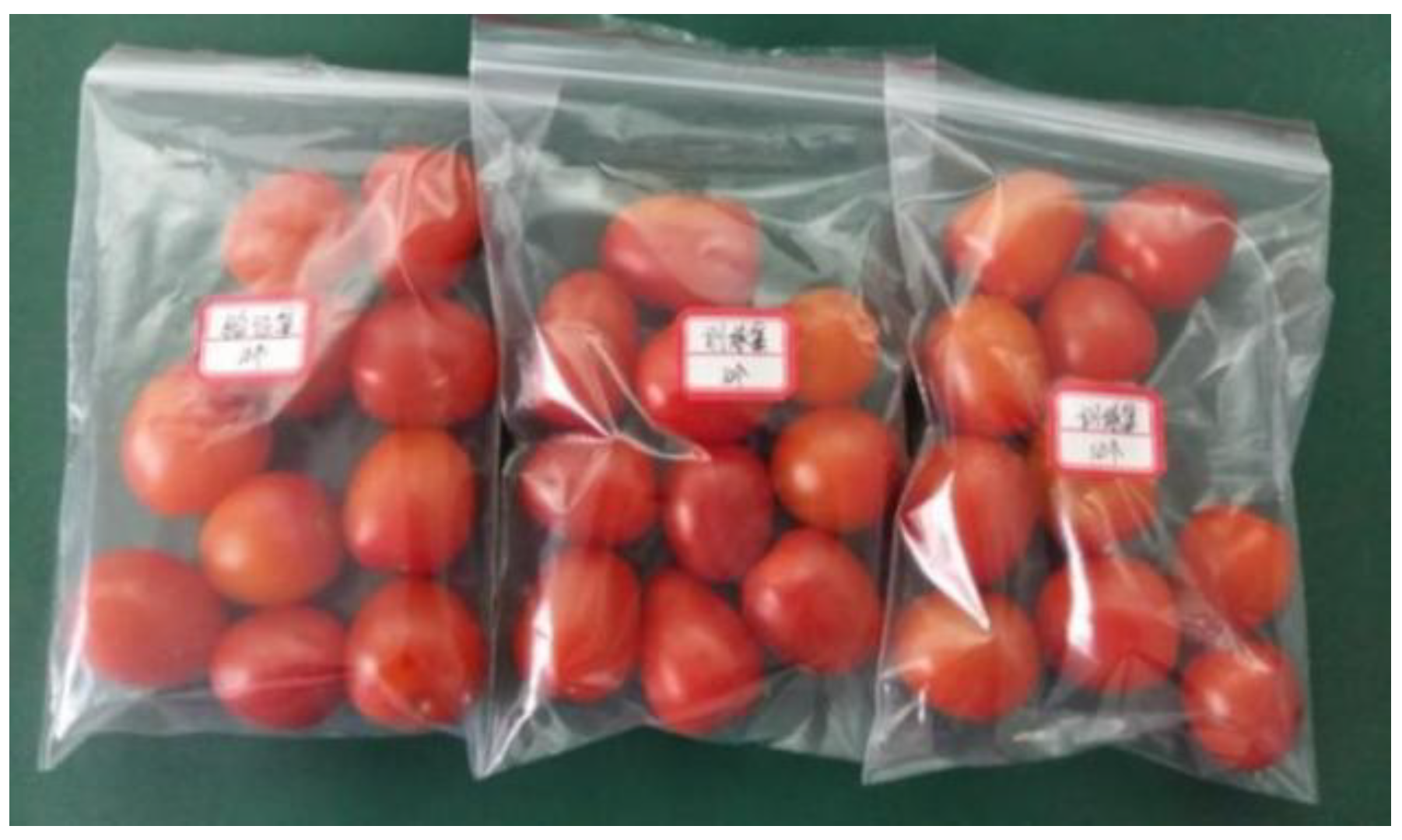Non-destructively determining the sugar content of cherry tomatoes is always a difficult problem [16]. As cherry tomatoes are rich in nutrition, this fruit is very popular. Therefore, this paper took cherry tomatoes as the samples to study the related sections.

As a new non-destructive testing technology, near-infrared spectroscopy has broad application prospects in agriculture, food, and other fields [17,18,19,20]. As a fast, non-destructive, and efficient detection method, near-infrared spectroscopy can be used to analyze the physicochemical properties of all samples related to hydrogen radicals. NIR spectroscopy also enables rapid qualitative or quantitative analyses of specific components. Therefore, near-infrared technology can be considered for the non-destructive testing and detection analyses of fruits [11,12].

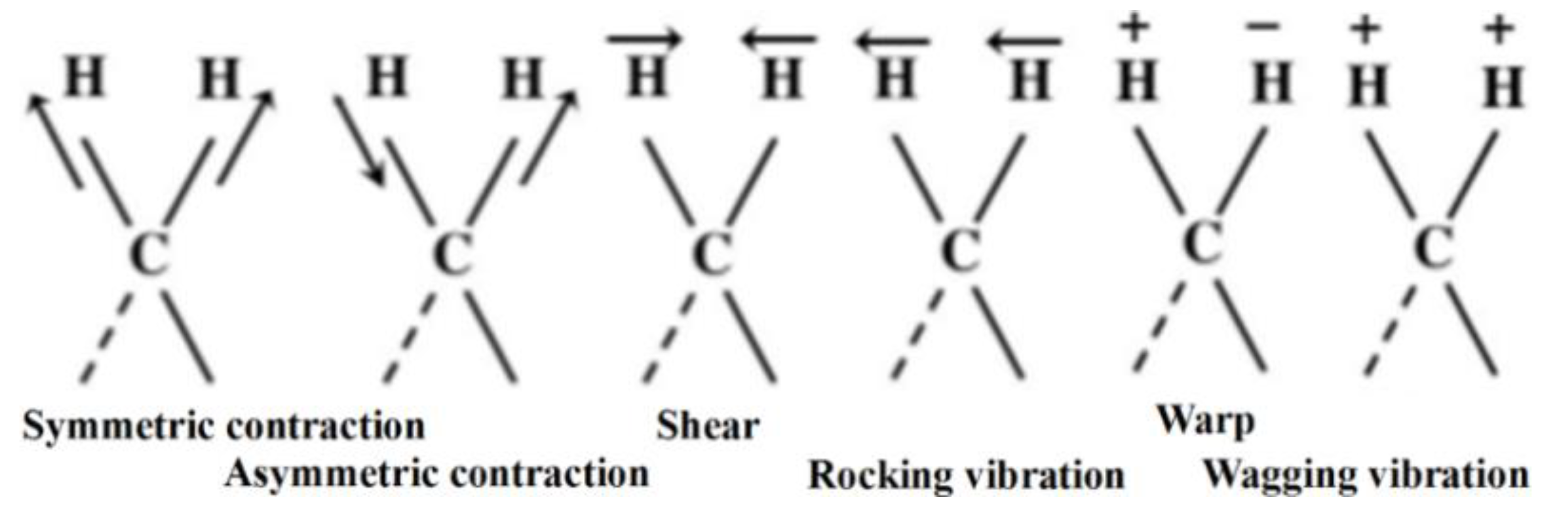
The NIR spectrum is mainly caused by the non-resonance of molecular vibrations. This leads to the oscillation of molecular vibrations from the ground state to a higher energy level. When molecules change from one excited state to another, they produce frequency-multiplying absorptions and combined frequency absorptions because of the absorptions at different fundamental frequencies [21]. Near-infrared spectroscopy mainly reflects the frequency-doubled and total-frequency absorption information for hydrogen-containing groups (O-H, C-H, N-H, S-H, P-H) [22]. When a molecule is exposed to infrared radiation, it is excited into resonance and the light’s energy is partially absorbed. We can measure the absorption of light and obtain an extremely complex spectrum that represents the properties of the substance [23]. Examples of stretching vibrations and deformation vibrations of the measured material molecules are shown in Figure 1. With the appropriate stoichiometry, the near-infrared absorption spectrum may be related to the substance’s composition or properties, and a corresponding model can be established.

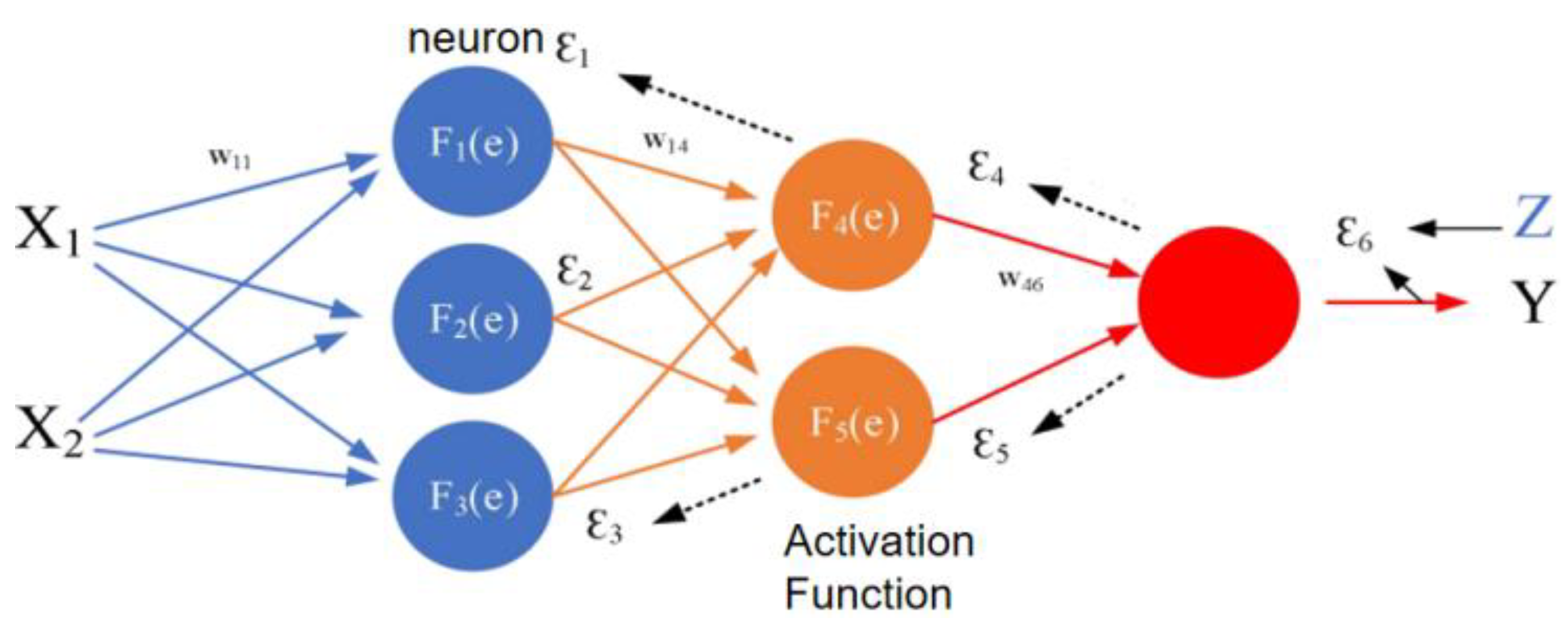
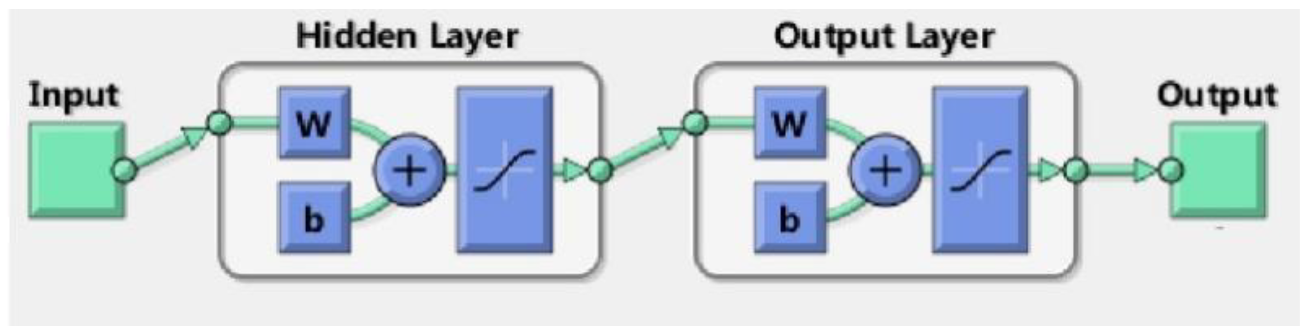
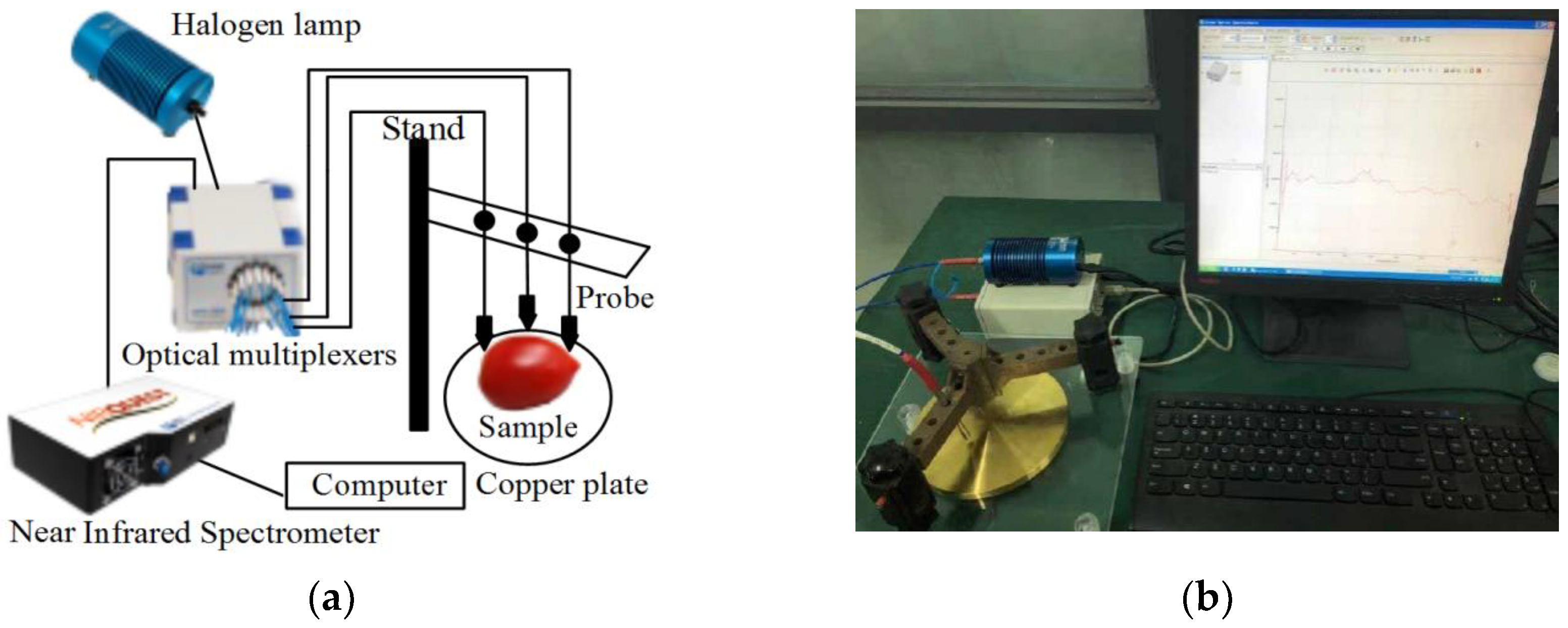
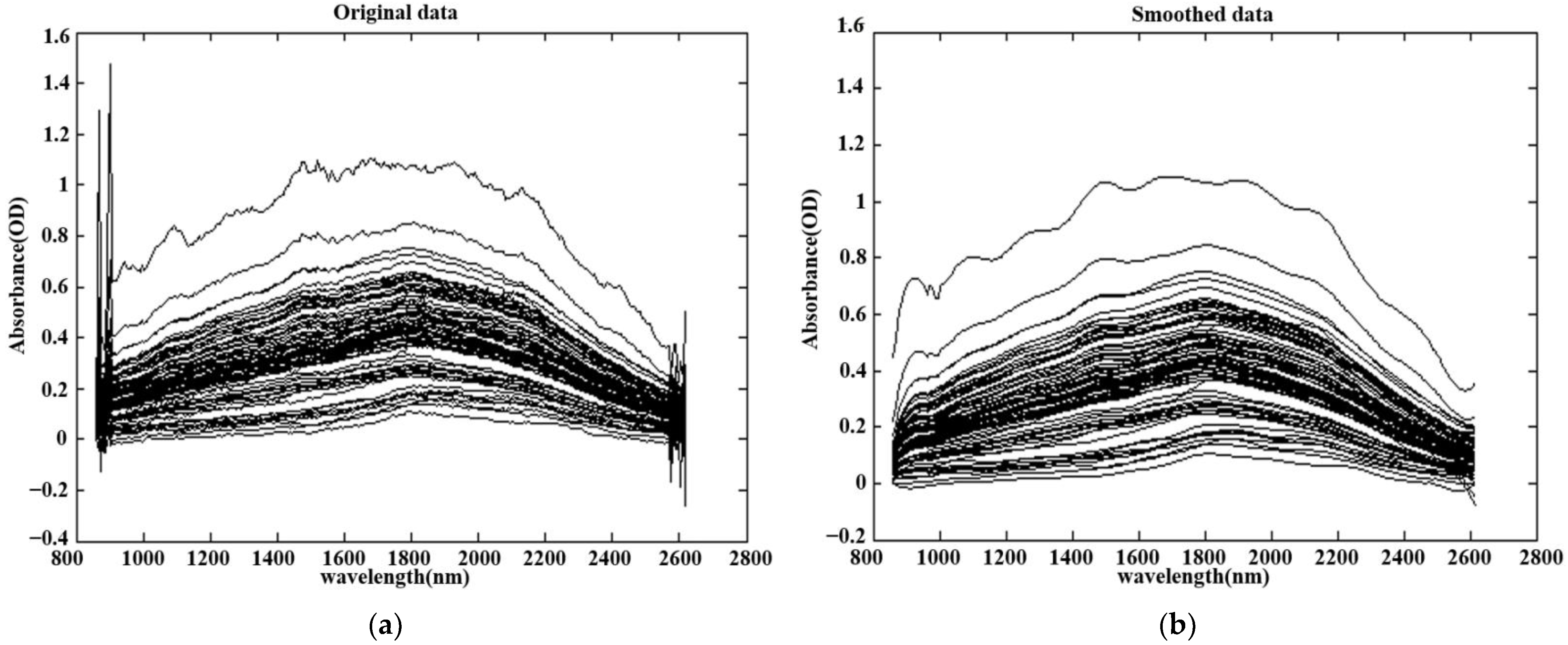
An intelligent near-infrared diffuse reflectance spectroscopy (INIS) method for the non-destructive testing of the sugar content in vegetables and fruits was designed on the basis of a near-infrared spectrum analysis technique. In the experimental part, cherry tomatoes were selected as the representative samples and a BP network model was established to study the sugar content. Spectral features were extracted from experimental the spectral data using smoothing and a principal component analysis (PCA). An intelligent near-infrared diffuse reflectance spectroscopy scheme (INIS) was the proposed for the non-destructive detection and prediction of the sugar content in the representative fruit.

The BP neural network technology has broad application prospects in near-infrared non-destructive testing, and the prediction results are more accurate. In fruit detection, qualitative and quantitative analyses can be carried out on the fruits, including to assess the fruit types, regional classifications, fruit sugar contents, and so on. However, there is room for improvement in the accuracy of the results, and many fruits remain to be studied. Therefore, this paper combines near-infrared spectroscopy and a BP neural network to study the sugar content of cherry tomatoes and to improve the accuracy of the results.

The remainder of this paper is organized as follows. Section 2 gives a brief introduction to the present situation regarding the domestic and foreign research. In Section 3, we introduce the near-infrared spectroscopy technology, BP neural network, and model evaluation criteria. In Section 4, the experimental materials and methods are presented. In Section 5, we analyze and discuss the data collected from the experiments. In Section 6, we draw conclusions and describe the future outlook.

2. The Related Work

As a new non-destructive testing technology, near-infrared spectroscopy has broad application prospects in agriculture, food, and other fields.

Ref. [24] used visible near-infrared spectroscopy to predict soluble solids in Fuji apples. Ref. [25] used near-infrared spectroscopy to calibrate models of soluble solids and moisture content in Cucurbitaceae. Ref. [26] determined the chemical and sensory properties of tomatoes based on near-infrared spectroscopy. Ref. [27] used near-infrared spectroscopy for the non-destructive prediction of the total soluble solids in strawberries. Ref. [28] used near-infrared spectroscopy to improve the prediction of pear fruit moisture and soluble solid contents. Ref. [29] conducted a non-contact assessment of intact mangoes using NIR spectroscopy. According to the existing research on non-destructive testing and detection testing, near-infrared spectroscopy technology could be used for the non-destructive testing of the sugar content of cherry tomatoes [30,31].

An artificial neural network (ANN) is a mathematical model that simulates animal neural networks and performs distributed parallel information processing. Such networks depend on the complexity of the system. The purpose of processing information is achieved by adjusting the mutual relationship between a large number of internal nodes. ANNs have the self-learning ability to adapt and have been connected with machine learning [32], big data [33], automatic processing [34], analytics [35], and algorithms [36].

Ref. [37] proposed a new method involving NIR-HSI combined with PLS. Ref. [38] examined the FOS content in sun-dried banana syrup using NIR measurements. The PLS results indicated that the optimized wavelength range is better than the full wavelength. Ref. [39] showed that VIS/NIR spectroscopy could be used to classify three varieties of tomatoes, as well as to determine their quality parameters, such as their SSC, TA, taste (SSC/TA), and firmness. Ref. [40] used a PLS regression and wavenumber selections to perform non-destructive FT-NIR measurements and prediction models of texture. The results were that the R² values ranged from 0.70 to 0.97 and the RPD values from 1.8 to 6.1. Ref. [41] used tropical papaya fruit as a raw material to produce pulp products. Based on a BP neural network, he predicted and verified the processing conditions for papaya pulp and meat products. The results showed that the products produced under certain conditions meet health and safety standards. Ref. [42] established a model through a BP neural network and then combined this with near-infrared spectroscopy technology to predict the sugar content of cherry tomatoes. The results showed that this method can reasonably predict the sugar content.

In order to achieve the fast and non-destructive detection of the internal quality of cherry tomatoes, Refs. [43,44] established a cherry tomato transmission detection system. The correlation analysis and normalization treatment were used to correct the diameter of the cherry tomatoes. A rapid and non-destructive study was carried out on the soluble solid content (SSC) of cherry tomatoes based on this system. The results showed that the visible/near-infrared transmission spectrum combined with the normalization of the fruit diameter can be used to effectively predict the internal quality of cherry tomatoes and eliminate the errors caused by different fruit diameters. According to the existing research on the non-destructive testing [30] of cherry tomatoes, artificial neural networks maybe good tools to resolve the problem.

Based on the previous research, we finished a literature review [30], basic theory study, near-infrared diffuse reflection experiment, integrated environment experiment [12], typical fruit selection experiment, typical fruit spectrum data collection study [45], and a spectral data analysis of typical fruits. Based on the neural network design, we designed an intelligent near-infrared diffuse reflectance spectroscopy (INIS) scheme for the non-destructive testing of the sugar contents in fruits [12].

Ref. [46] proposed a weighting mechanism to connect samples with dictionary atoms. At the same time, traditional dictionary learning methods are prone to overfitting for patient classification with limited training datasets. Ref. [45] introduced artificial neural networks based on a 1-D CNN (one-dimensional convolutional neural network) and Bi-LSTM (bidirectional long and short-term memory). Abstract features of different properties are obtained through preprocessed sensory data. Ref. [47] proposed a new deep learning architecture called the recurrent 3D convolutional neural network (R3D). It is used to extract valid and discriminative spatiotemporal features for action recognition. This enables the capture of long-range time information by aggregating 3D convolutional network entries as inputs to LSTM (long short-term memory) architectures.

There are many known neural network algorithms, and each algorithm has its own characteristics. After reviewing the research status at home and abroad, it was found that BP algorithms can be used in the detection of many kinds of fruit, but the use of a BP neural network to predict the content of virgin fructose has great advantages. Therefore, in the next experiments, we choose the BP algorithm.

3. INIS Scheme

In this paper, we propose an intelligent near-infrared diffuse reflectance spectroscopy (INIS) scheme for the non-destructive testing of the sugar contents in vegetables and fruits. In the experimental part, we select the cherry tomato as the representative fruit. However, this method can be extended and optimized to be used in almost all fruits and vegetables.

3.1. Basic Principles and Characteristics of Near-Infrared Spectroscopy Technology

Near-infrared light refers to the electromagnetic waves in the wavelength range of 780–2526 nm, which are generally divided into two regions: near-infrared short waves and long waves. The wavelengths corresponding to various electromagnetic waves are shown in Figure 2.

The near-infrared detection methods for fruit sugar content include near-infrared reflection detection, near-infrared transmission detection and near-infrared diffuse reflection detection. A schematic diagram of the near-infrared reflection detection, near-infrared transmission detection, and near-infrared diffuse reflection detection methods is shown in Figure 3.

A comparison of the applicable objects and characteristics of the three main methods of near-infrared detection is shown in

Table 3. Three main infrared detection technologies.

Near-Infrared Spectrometric Method	The Applicable Objects	The Characteristics
transmission detection	Transparent and semitransparent sample	It can fully reflect the internal structure information of the sample, but needs high energy specific light source.
reflection detection	Opaque, solid, and semisolid sample	According to the regular reflected light, reflected light mainly carries the spectral information of the surface of the fruit, while the internal information of the fruit is less.
diffuse reflection detection	Opaque, solid, and semisolid sample	It can fully reflect the internal structure information of the sample, but does not need high energy specific light source.

.

As shown in Table 3, the near-infrared reflectance detection method is more suitable for experimental research on the detection of fruit peel surface information. The near-infrared transmission method basically reflects the internal quality information of the fruit, but it requires a specific light source with high energy. In the near-infrared diffuse reflection detection method, the light information received by the detector not only reflects the characteristics of the internal tissue of the fruit, but it also has relatively low requirements for the light source. No specific high-energy light source is required for detection. Therefore, this experiment is based on the advantages and disadvantages of the three NIR detection methods and various factors in the test design. In the end, it was decided to use the near-infrared diffuse reflection detection method.

3.2. The BP Neural Network Establishment

3.2.1. BP Neural Network

The term backpropagation and its general use in neural networks was announced by Rumelhart, Hinton, and Williams in 1986. It is a one-way propagation multi-layer forward network, which is trained using the error back propagation method [37]. BP neural networks have many application scenarios [48].

The BP network is composed of an input layer, hidden layer, and output layer. Each layer is composed of a number of simple neurons that operate in parallel. The neurons in the network layer are completely interconnected, and the neurons of the same level are not interconnected. Although the structure of each neuron is relatively simple and has only limited functions, the network system composed of a large number of neurons can achieve extremely rich and colorful functions. In the topology of the BP network, the input layer and output layer can be obtained from the problem itself. The number of nodes in the hidden layer is the key.

The topological structure of the BP neural network is shown in Figure 4. Its learning rule adopts a gradient descent algorithm. At first, the input vector is passed positively to the hidden layer. Then, the transfer function is calculated, and finally the result is passed to the output layer and the output result is obtained [49]. The BP network changes the weights and thresholds through forward feedback errors. When the network output and actual expected output for the mean square error are below a certain threshold or the number of learning points meets certain conditions, the BP neural network training is completed.

Each hidden layer contains multiple neurons. The neuron format is shown in Figure 5. The numbers of input X and output Y are set as required, but X₀ is the specified value of −1. Each input corresponds to a weight, and X₀ corresponds to w₀θ. In the calculation process, the sum is calculated first and then the mapping is performed.

Here, X is the input,$X=\left[X_0,X_1,\dots ,X_n\right]$, W is the weight,$\mathrm{W}=\left[\begin{array}{c}{\mathrm{w}}_{\mathrm{i}0}\\ {\mathrm{w}}_{\mathrm{i}1}\\ ⋮\\ {\mathrm{w}}_{\mathrm{in}}\end{array}\right]$, and Y is the output. The output can be represented as Equation (2):

$$ne{t}_{\mathrm{i}}={\displaystyle \sum }_{\mathrm{j}=1}^{\mathrm{n}}{\mathrm{W}}_{\mathrm{ij}}{\mathrm{X}}_{\mathrm{j}}-\theta =\mathrm{XW}$$

(1)

$$y_i=f\left(ne{t}_{\mathrm{i}}\right)=\mathrm{f}(\mathrm{XW})$$

(2)

In this way, the calculation of one neuron is completed. The reference for the construction of the entire BP neural network model is shown in Figure 6. The result for each layer of neurons is the sum of the products of the previous layer and the weights. We continue in turn until the predicted value Y is output, and then compare it with the actual value. An error ε₆ is generated. F₆(e) pushes the error backwards. The errors ε₄ and ε₅ are formed in F₄(e) and F₅(e) in turn. The backward calculation of the error is shown in Equations (3) and (4). Here, Z is the measured value and Y is the predicted value:

$${\epsilon }_4={\mathrm{W}}_{46}{\epsilon }_6$$

(3)

$${\epsilon }_1={\mathrm{W}}_{14}{\epsilon }_4+{\mathrm{W}}_{15}{\epsilon }_5$$

(4)

In this way, the errors for all levels are calculated backward in turn. Then, we start from the first layer to adjust the weights of all levels to reduce the errors. Then, we calculate forward and repeat the operation until the error for the actual value is between the set value. At this point, the constructed model is the established BP neural network model. The number of neurons in the model and the setting of the training function are the keys to ensuring the accuracy of the model.

3.2.2. The Establishment of BP Neural Network Model

The structure of the network includes an input layer, hidden layer, and output layer. In this paper, the preprocessed principal component data are used as the inputs for the BP neural network, and the measured sugar content of the cherry tomatoes is the target output of the network. The number of neurons in the hidden layer is determined by the following empirical formula. The structure of the BP neural network is constructed by using the neural toolbox from MATLAB software. The system structure diagram is shown in Figure 7.

The empirical formula is:

$${\mathrm{n}}_1=\sqrt{n+m}+k$$

(5)

Among them, n₁ is the number of neurons in the hidden layer, n is the number of input layer nodes, m is the dimension of the output layer, and k is a positive integer of 1~10.

The number of neurons in the hidden layer can be calculated by the empirical formula for four randomly selected values. Since the value of k is a positive integer from 1 to 10, the resulting number of neurons in the hidden layer is a range. The calculation results are shown in

Table 4. BP neural network calculation of the number of neurons in the hidden layer.

a	16	23	31	81
number of neurons	√7 + k	√24 + k	√32 + k	9 + k
range of neurons	5~14	5~15	5~16	10~19

.

The training function, adaptive learning function, performance parameters, and hidden layer transfer function settings in the BP network function are shown in

Table 5. BP neural network calculation of the number of neurons in the hidden layer.

Network Parameters	Parameter Setting
Training function	Trainlm
	Traindgm
	Trainscg
Adapting learning function	Learngdm
Performance function	MSE
Transfer function	Tansig

. The training functions of the network include Trainlm, Traindgm, and Trainscg. The most suitable training function is selected through the results of the later model building process.

The specific parameter settings in the BP network training process are shown in

Table 6. BP neural network model parameter settings.

Network Parameters	Parameter Settings
Epochs	1000
Goal	0
Show	25
Max fail	6
Min grad	1 × 10−7

. Among them, the number of iterations can be set to a small number first, and then one can observe the convergence result. If the convergence curve of the results window decays faster, the previous parameters are more effective. Therefore, a larger number can be filled-in to make the network converge, otherwise the previous parameters are modified.

3.2.3. The Evaluation Criteria of the Model

In this paper, the cross-validation determination coefficient (R²) and average absolute deviation (MAE) are used as the evaluation criteria for the model [50]. The specific formulas are shown as follows:

$$R^2=\frac{{\displaystyle {\sum }_{i=1}^{\mathrm{n}}{({\mathrm{y}}_{iP}-y_m)}^2}}{{\displaystyle {\sum }_{i=1}^{\mathrm{n}}{({\mathrm{y}}_{im}-y_m)}^2}}$$

(6)

$$MAE=\frac{1}{n}{\displaystyle {\sum }_{i=1}^n(\left|y_{ip}-y_{im}\right|)}$$

(7)

Regarding Equations (6) and (7), y_ip is the predicted value of sugar, y_im is the measured value, and y_m is the average value of the measured value. The cross-validation determination coefficient is close to 1, and the smaller the MAE, the better the model predictability.

3.3. INIS Architecture

The INIS model mainly includes the following two processes: (1) finding the relationship between the near-infrared spectrum and the properties of the measured substance through the sample and establishing a model; (2) predicting the properties of the substance under testing through the established model. These two processes are the correction model and the predictive model. In Figure 8, the process of the modeling is shown on the left and the process of predicting the model is shown on the right. It can be seen that the INIS model mainly includes three parts: near-infrared spectroscopy acquisition, model application, and stoichiometry. Only through the combination of these three parts can a rapid and accurate analysis effect be achieved.

An optimal model cannot be established overnight, but an optimal model can be obtained through a continuous cycle of test–trial and build–test–comparison phases. After ensuring the stability of the model, we can get a more accurate prediction result.

4. Materials and Methods

4.1. Materials

Near-infrared spectroscopy is usually divided into three acquisition methods: transmission, diffuse reflection, and diffuse transmission. Among them, diffuse reflection spectroscopy is more suitable for solids [51].

We carefully selected 80 cherry tomatoes (each of uniform color, a similar size, and surface-damage-free) in supermarkets as research samples. We first washed the 80 cherry tomatoes to remove surface stains and impurities. Then, dried the surfaces of the cherry tomatoes. Finally, we placed groups of 10 cherry tomatoes into 8 bags and stored them at room temperature. The samples of cherry tomatoes are shown in Figure 9.

The three points along the equator (approximately 120° apart) of the cherry tomato were taken as data collection points, as shown in Figure 10.

In the experimental part, although we selected the cherry tomatoes as the representative only, this method can be extended and optimized to be used in almost all fruits and vegetables.

4.2. Laboratory Apparatus

The experimental instruments included a halogen lamp, near-infrared spectrometer, MPM-2000 optical multiplexer, stand, horizontal ball, copper plate, black box, and computer. The parameters of the experimental instruments are shown in

Table 7. The parameters of the experimental instruments.

Experimental Instruments	Parameter
Halogen lamp (HL-2000-HP)	Wavelength range	360–2400 nm
	Output power	8.8 mW
	Integration time	1–400 ms
Near-Infrared Spectrometer (NIR 256-2.5)	Wavelength range	900–2500 nm
	Slit length	25 µm
MPM-2000 optical multiplexers	Wavelength range	250–800 nm
	Materials	Copper
Sugar Meter	Range	0–80%Brix
	Materials	Brass H62
Copper plate	Diameter	200 mm
	Thickness	15 mm

.

The spectral acquisition software is developed by Ocean Optics of the United States, which has spectral acquisition mode settings, spectral parameter settings, and spectral acquisition and spectral viewing functions.

4.3. Measurement Methods

The experimental system uses a tungsten halogen lamp as the light source. The probe is closely attached to the surface of the cherry tomato, and the near-infrared light is transmitted to the surface of the cherry tomato through the optical multiplexer. After the interaction between the near-infrared light and the fruit, the internal structure and information relating to the fruit are transmitted to the spectrometer through the diffuse reflection. Finally, the collected spectral data are stored in the computer. The structure of the experimental system and the field demonstration are shown in Figure 11.

5. Performance Analysis and Discussion

5.1. Spectral Pretreatment

5.1.1. Smoothing

Due to human operation and the external environment, the spectral data will not only contain the internal structural information for the sample, but will also contain some redundant information and noise. These factors will affect the accuracy of the results. Therefore, it is very important to achieve spectral noise reduction. Signal smoothing is a relatively common method for eliminating noise. The noise in the spectrum is assumed to be zero random white noise. The use of multiple measurements to create an average may reduce the noise and increase the signal-to-noise ratio.

The Savitzky–Golay convolutional smoothing algorithm is an improvement on the movement smoothing algorithm. Let the width of the filter window be n = 2m + 1 and each measurement point be x = (−m, m + 1, 0...0, 1....m − 1, m). The k−1 polynomial is used to fit the data points within the window. The polynomial is $\mathrm{y}=a_0+a_{1}x+a_2{x}^2+\dots +a_{k-1}{x}^{k-1}$.

Thus, there are n such equations, forming a system of k-element linear equations. To ensure the system of equations has a solution, n should be greater than or equal to k, so generally n > k is selected. The fitting parameter A is determined by the least-squares method. This results in a system of k-element linear equations. This is shown in Equation (8):

$$\left(\begin{array}{c}{y}_{-m}\\ y_{-m-1}\\ ⋮\\ y_m\end{array}\right)=\left(\begin{array}{cccc}1& -m& \cdots & {(-m)}^{k-1}\\ 1& -m+1& \cdots & {(-m+1)}^{k-1}\\ ⋮& ⋮& ⋮& ⋮\\ 1& m& \cdots & m^{k-1}\end{array}\right)\left(\begin{array}{c}{a}_0\\ a_1\\ ⋮\\ a_{k-1}\end{array}\right)+\left(\begin{array}{c}{e}_{-m}\\ e_{-m+1}\\ ⋮\\ e_m\end{array}\right)$$

(8)

The above equation can be expressed as $Y_{(2m+1)\times 1}=X_{(2m+1)\times k}\cdot A_{K\times 1}+E_{(2m+1)\times 1}$ in the matrix form. The least-squares solution A is $\dot{A}={\left(X^{\mathrm{T}}\cdot X\right)}^{-1}\cdot X^{\mathrm{T}}\cdot Y$. The model-predicted value or filter value Y is $\widehat{Y}=X\cdot A=X\cdot {\left(X^{\mathrm{T}}\cdot X\right)}^{-1}\cdot X^{\mathrm{T}}\cdot Y=B\cdot Y$.

The Savitzky–Golay algorithm is a smoothing filtering algorithm that is not restricted by the sample data and is suitable for the smooth de-noising of all kinds of signals. Compared with other traditional algorithms, the smoother denoising effect of the Savitzky–Golay algorithm has more stability and less error [52]. Therefore, the Savitzky–Golay algorithm is used in this paper for smooth denoising. As shown in Figure 12, the noise is basically removed after the smoothing process, and the peaks in the spectrum are not significantly distorted or lost.

5.1.2. Principal Component Analysis

In the prediction of sugar content, there are many factors that affect the results and have certain correlations. Moreover, too many inputs can also influence the precision of the forecast model. So the PCA is adopted to solve the problem.

The principal component analysis method recombines many original indicators with a certain correlation into a set of new linearly independent comprehensive indicators. It is a multivariate mathematical statistics method that converts multiple indicators into a few comprehensive indicators. The comprehensive index not only simplifies the complex issues, but also retains most of the information for the original indicators [53,54,55].

The principal component analysis not only eliminates the redundancy between data, but also preserves the main information for the original variable, and the two variables are independent of each other. At the same time, the purpose of simplifying the dimensions of the input variable is achieved. In other words, all of the original variables are replaced with a small number of variables and most of the original data are overwritten.

The magnitude of the eigenvalue represents the contribution degree of the corresponding eigenvector to the whole matrix after orthogonalization. The principal component contribution rate refers to the proportion of the variance that a principal component can explain to the total variance, and the larger the value, the stronger the ability of the principal component to synthesize the information of the original variable. When the cumulative contribution rate is close to 1, the first p indicator variables $y_1,y_2,\cdots ,y_p$ are p principal components, instead of the original m indicator variables, so that the p principal components can be comprehensively analyzed. As shown in

Table 8. The principal component analysis results.

Principal Component Information	Contribution Rate/%	Cumulative Contribution Rate/%
0.9407468	97.267704	97.267704
0.0209914	2.1703883	99.4381
0.003511	0.3630201	99.8011
0.0008316	0.0859785	99.8871
0.000231	0.0238872	99.911
0.0002125	0.0219725	99.933
0.0001433	0.0148213	99.9478
0.0001204	0.0124535	99.9602
8.06 × 10−5	0.0083345	99.9686
5.78 × 10−5	0.0059718	99.9745
5.01 × 10−5	0.0051796	99.9797
3.83 × 10−5	0.0039625	99.9837
3.24 × 10−5	0.003353	99.987
2.59 × 10−5	0.0026766	99.9897
1.97 × 10−5	0.0020354	99.9917
1.81 × 10−5	0.0018685	99.9936
1.57 × 10−5	0.0016231	99.9952
1.37 × 10−5	0.0014145	99.9966
8.82 × 10−6	0.0009118	99.9976
6.52 × 10−6	0.0006744	99.9982
5.01 × 10−6	0.0005178	99.9987
3.71 × 10−6	0.0003836	99.9991
2.53 × 10−6	0.0002615	99.9994
1.55 × 10−6	0.0001601	99.9996
1.26 × 10−6	0.0001301	99.9997
6.05 × 10−7	6.26 × 10−5	99.9997
3.70 × 10−7	3.82 × 10−5	99.9998
3.16 × 10−7	3.26 × 10−5	99.9998
2.48 × 10−7	2.56 × 10−5	99.9998
2.33 × 10−7	2.41 × 10−5	99.9999
1.84 × 10−7	1.91 × 10−5	99.9999
1.36 × 10−7	1.40 × 10−5	99.9999
1.17 × 10−7	1.21 × 10−5	99.9999
9.03 × 10−8	9.34 × 10−6	99.9999
8.97 × 10−8	9.27 × 10−6	99.9999
7.63 × 10−8	7.89 × 10−6	99.9999
7.31 × 10−8	7.56 × 10−6	99.9999
6.00 × 10−8	6.20 × 10−6	100
5.01 × 10−8	5.18 × 10−6	100
4.65 × 10−8	4.81 × 10−6	100
3.82 × 10−8	3.95 × 10−6	100
3.20 × 10−8	3.30 × 10−6	100
3.09 × 10−8	3.19 × 10−6	100
2.59 × 10−8	2.68 × 10−6	100
2.17 × 10−8	2.24 × 10−6	100
2.07 × 10−8	2.14 × 10−6	100
1.81 × 10−8	1.87 × 10−6	100
1.76 × 10−8	1.82 × 10−6	100
1.61 × 10−8	1.67 × 10−6	100
1.46 × 10−8	1.50 × 10−6	100
1.34 × 10−8	1.38 × 10−6	100
9.74 × 10−9	1.01 × 10−6	100
9.48 × 10−9	9.81 × 10−7	100
8.92 × 10−9	9.23 × 10−7	100
7.92 × 10−9	8.19 × 10−7	100
7.14 × 10−9	7.38 × 10−7	100
6.36 × 10−9	6.58 × 10−7	100
6.19 × 10−9	6.40 × 10−7	100
5.86 × 10−9	6.06 × 10−7	100
4.75 × 10−9	4.91 × 10−7	100
4.57 × 10−9	4.72 × 10−7	100
4.14 × 10−9	4.28 × 10−7	100
3.52 × 10−9	3.64 × 10−7	100
3.21 × 10−9	3.32 × 10−7	100
2.80 × 10−9	2.89 × 10−7	100
2.60 × 10−9	2.68 × 10−7	100
2.50 × 10−9	2.58 × 10−7	100
2.33 × 10−9	2.41 × 10−7	100
2.12 × 10−9	2.19 × 10−7	100
2.02 × 10−9	2.09 × 10−7	100
1.86 × 10−9	1.93 × 10−7	100
1.52 × 10−9	1.57 × 10−7	100
1.47 × 10−9	1.52 × 10−7	100
1.41 × 10−9	1.46 × 10−7	100
1.17 × 10−9	1.21 × 10−7	100
9.93 × 10−10	1.03 × 10−7	100
9.25 × 10−10	9.56 × 10−8	100
8.79 × 10−10	9.09 × 10−8	100
7.05 × 10−10	7.29 × 10−8	100
5.79 × 10−10	5.99 × 10−8	100

, the spectral data are the principal component characteristic roots, principal component contribution rates, and cumulative contribution rates after the principal component analysis.

By performing a principal component analysis on the preprocessed spectral data, removing redundant information, and screening out the characteristic factors, the smoothed absorption data matrix (25,80) is reduced to (80,80). In the end, the 256 absorption data for a single cherry tomato were reduced to 80 characteristic factors.

According to the cumulative contribution rate of the principal component analysis in

Table 9. Some of the principal component analysis results.

a	Principal Component Information	Contribution Rate/%
16	0.000018071150535	99.9936
23	0.000002528971721	99.9994
31	0.000000844258438	99.9999
80	0.000000000579484	100

, four datapoints with a cumulative contribution rate higher than 99.99% were randomly selected, including one with a cumulative contribution rate of 100 (see Table 9). In the table, there is a reference to the principal component; that is, the number of rows of the matrix input of the selected network.

The input layer dimension n = a (16/23/31/80), and the number of neurons in the hidden layer can be calculated by Equation (5). Since the k value is a positive integer in the range of 1 to 10, the number of neurons in the hidden layer is a range. The calculation results are shown in

Table 10. Calculation of the layer neurons.

a	n1	r Range
16	√7 + k	5–14
23	√24 + k	5–15
31	√32 + k	5–16
80	9 + k	10–19

.

The input layer dimension n = a (16/23/31/80). The number of hidden layer neurons n1 can be obtained from Table 8. The dimension of the output layer is m = 1. The network training function is trainlm/traindgm/trainscg. Therefore, we get 12 prediction figures.

According to the results for the above training function Trainlm, when a = 80 and the number of neurons is 12, the average absolute deviation is the smallest, and the cross-validation determination coefficient is not the largest but it is similar to the cross-validation determination coefficient of the average absolute deviation of the second hour (a = 31), so for the training function Trainlm, when a = 80 and the number of neurons is 12, the model has the best prediction effect. The cross-validation coefficient of determination is 0.8328 and the mean absolute deviation is 0.5711.

According to the result, when the training function is selected as Traindgm, when a = 80 and the number of neurons is 11, the average absolute deviation is the smallest, and the cross-validation coefficient of decision is small but it is close to 1, so for the training function Traindgm, when a = 80 and the number of neurons is 11, the model has the best prediction effect. The coefficient of decision for cross-validation is 0.8096, and the mean absolute deviation is 0.8751.

According to the results for the above training function Trainscg, when a = 80, the number of neurons is 11, the average absolute deviation is the smallest, and the cross-validation coefficient of determination is the second person, which is close to 1, so for the training function selection Trainscg, when a = 80 and the number of neurons is 11, the model has the best prediction effect, the cross-validation determination coefficient is 0.7417, and the average absolute deviation is 0.6403.

5.2. BP Network Model Analysis

The learning process for the BP neural network consists of two parts: forward propagation and error backpropagation. Input sampling signals are sent in sequence by input, hidden, and output layers [56]. The input of the network is the spectral data after the principal component analysis. The output is the sugar content of the cherry tomatoes.

According to

Table 11. Model prediction results.

a	Network Training Function	n1	R2	MAE
16	Trainlm	10	0.8787	0.8946
	Traingdm	13	0.9249	0.9749
	Trainscg	12	0.5172	0.8672
23	Trainlm	11	0.9901	0.9716
	Traingdm	11	0.9211	0.9539
	Trainscg	13	0.8103	0.7310
31	Trainlm	6	0.8299	0.6371
	Traingdm	10	0.9044	0.9697
	Trainscg	11	0.4348	0.8079
80	Trainlm	12	0.8328	0.5711
	Traingdm	11	0.8096	0.8751
	Trainscg	11	0.7417	0.6403

and Figure 13, when a = 80, the network training function is Trainlm, and the number of hidden layer neurons is 12, the cross-validation determination coefficient R² is 0.8328 and the average absolute deviation is 0.5711. Therefore, the model described above is the best and the prediction result is shown in Figure 13 (80-Trainlm).

6. Conclusions and Future Work

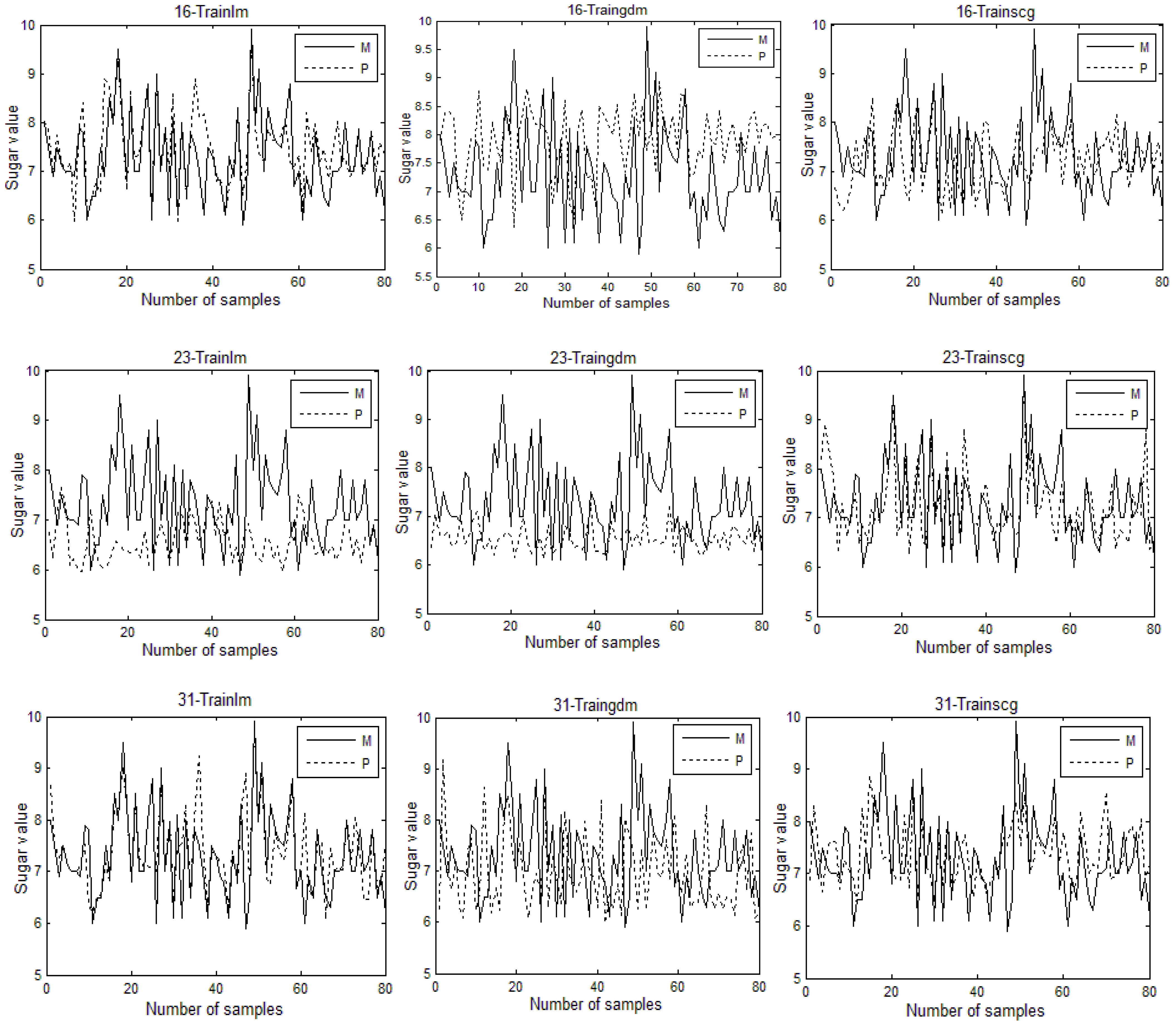
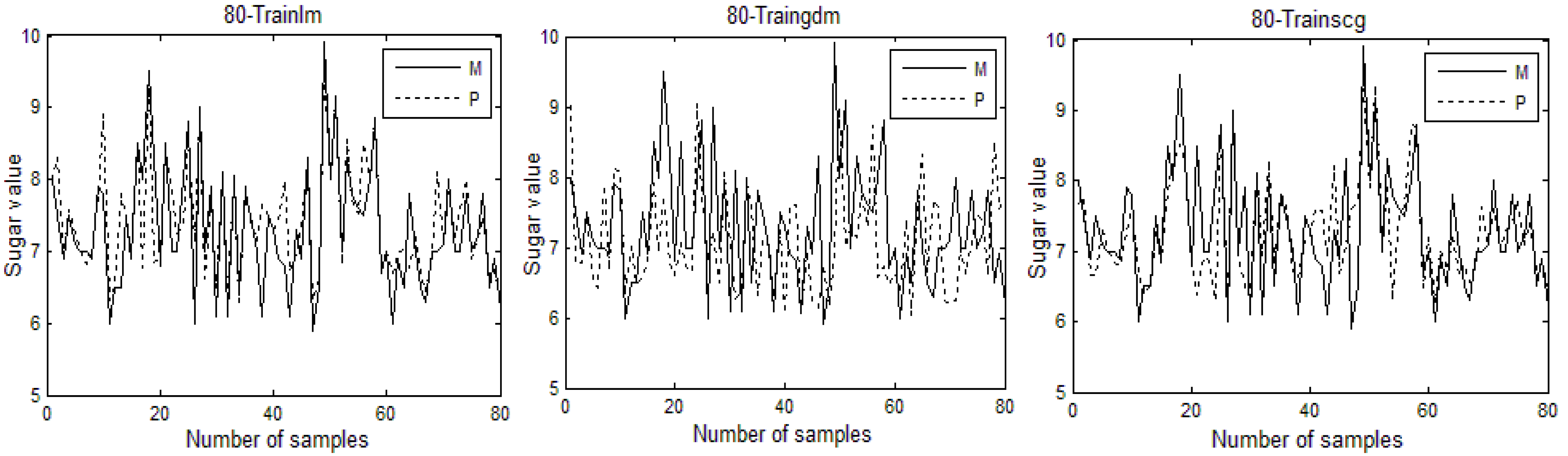
In this study, a near-infrared non-destructive testing method for the sugar content of cherry tomatoes was designed based on a BP neural network. An experimental system for near-infrared non-destructive testing was set up. The spectral data were preprocessed using the Savitzky–Golay algorithm and the principal component analysis method. The present study aimed to analyze the model prediction effects of the different parameters and to find the best model. The results show that when the network model structure of 80-12-1 is established and the network is trained using the training function Trainlm, the cross-validation determination coefficient of the model is 0.8328 and the average absolute deviation is 0.5711. Therefore, the model prediction effect is the best at this time.

The near-infrared non-destructive testing method based on the BP neural network proposed in this paper not only achieves the detection of the sugar content of cherry tomatoes, but also provides a foundation for the quality detection of cherry tomatoes, as well as for the quality detection of various other fruits and for fruit grading. However, the experimental process and the measurement of the sugar content will produce a certain error, and these errors will directly affect the accuracy of the results. Therefore, the challenge of reducing errors needs further research. In addition, due to the important role of fruit quality testing and grading in the agricultural field, a stable detection method that applies to all fruits is also a direction that needs to be studied.

In this paper, we selected the cherry tomato as the representative fruit. However, this method can be extended and optimized to be used in almost all fruits and vegetables. The optimal prediction model obtained in this paper is for cherry tomatoes. In order to improve the applicability of the model, other fruits can also be studied, so as to find the optimal prediction models for the sugar contents of a variety of fruits and to apply them in real life.

In this paper, the sugar content of cherry tomatoes was taken as the indicator to study the quality of the fruit. In addition, the indicators of fruit quality also included the acidity, PH value, and hardness, which can be combined to extract comprehensive indicators. Here, we have proposed a prediction model comprising comprehensive indicators and achieved comprehensive prediction results for fruit quality.

References

1. Ju, T. Research on the risk of fruit industry in western Yunnan. Eco-Econ. Rev. 2017, 1, 146–159. [Google Scholar]
2. Liu, G.; He, P.; Wang, Y. Agricultural ecological products and their value realization paths. J. Appl. Ecol. 2021, 32, 737–749. [Google Scholar]
3. Li, C.; Chen, J.; Zhu, J.; Luan, Z.; Zhang, Y.; Sun, G. Investigation and analysis on dietary nutrition of healthy centenarians in Hainan. Chin. Food Nutr. 2022, 28, 84–88. [Google Scholar]
4. Xia, F.; Hao, R.; Li, J.; Xiong, N.; Yang, L.; Zhang, Y. Adaptive GTS allocation in IEEE 802.15.4 for real-time wireless sensor networks. J. Syst. Archit. 2013, 59, 1231–1242. [Google Scholar] [CrossRef]
5. Kumar, P.; Kumar, R.; Srivastava, G.; Gupta, G.; Tripathi, R.; Gadekallu, T.; Xiong, N. PPSF: A Privacy-Preserving and Secure Framework Using Blockchain-Based Machine-Learning for IoT-Driven Smart Cities. IEEE Trans. Netw. Sci. Eng. 2021, 8, 2326–2341. [Google Scholar] [CrossRef]
6. Yao, Y.; Xiong, N.; Park, J.; Ma, L.; Liu, J. Privacy-preserving max/min query in two-tiered wireless sensor networks. Comput. Math. Appl. 2013, 65, 1318–1325. [Google Scholar] [CrossRef]
7. Zhao, J.; Huang, J.; Xiong, N. An Effective Exponential-Based Trust and Reputation Evaluation System in Wireless Sensor Networks. IEEE Access 2019, 7, 33859–33869. [Google Scholar] [CrossRef]
8. Zhang, W.; Zhu, S.; Tang, J.; Xiong, N. A novel trust management scheme based on Dempster–Shafer evidence theory for malicious nodes detection in wireless sensor networks. J. Supercomput. 2017, 74, 1779–1801. [Google Scholar] [CrossRef]
9. Huang, S.; Zeng, Z.; Ota, K.; Dong, M.; Wang, T.; Xiong, N. An Intelligent Collaboration Trust Interconnections System for Mobile Information Control in Ubiquitous 5G Networks. IEEE Trans. Netw. Sci. Eng. 2021, 8, 347–365. [Google Scholar] [CrossRef]
10. Wang, E.; Xiao, L.; Han, X.; Tan, B.; Luo, L. Design of an Agile Training System Based on Wireless Mesh Network. IEEE Access 2022, 10, 84302–84316. [Google Scholar] [CrossRef]
11. Fan, S. Detection of Apple Soluble Solids Based on Visible/Near-Infrared Spectroscopy and Imaging Technology. Ph.D. Thesis, Northwest China University of Agriculture and Forestry Science and Technology, Xianyang, China, 2016. [Google Scholar]
12. Liu, Q. Fruit Detection Research Based on Near-infrared Spectroscopy. J. Hubei Univ. Technol. 2018. [Google Scholar]
13. Panno, S.; Davino, S.; Caruso, A.; Bertacca, S.; Crnogorac, A.; Mandić, A.; Noris, E.; Matić, S. A Review of the Most Common and Economically Important Diseases that Undermine the Cultivation of Tomato. Crop in the Mediterranean Basin. Agronomy 2021, 11, 2188. [Google Scholar] [CrossRef]
14. Morais, P.; Ferreira, A.; Cruz, M.; Silva, F.; Nascimento, M.; Dias, N. Effect of Organic Residues as Fertilizer on Postharvest Quality of Cherry Tomatoes. Braz. Arch. Biol. Technol. 2021, 64. [Google Scholar] [CrossRef]
15. Zhang, J.; Zheng, F. Development trend of Chinese fruit production: 1978–2010. Xinjiang Agric. Reclam. Econ. 2013, 2, 31–34. [Google Scholar]
16. Qiao, X. Status quo, characteristics and trends of world fruit production. World Agric. 2010, 5, 37–41. [Google Scholar]
17. Dong, J.; Guo, W. Non-destructive determination of apple internal qualities using near-infrared hyperspectral reflectance imaging. Food Anal. Methods 2015, 8, 2635–2646. [Google Scholar] [CrossRef]
18. Guo, Y.; Ni, Y.; Kokot, S. Evaluation of chemical components and properties of the jujube fruit using near infrared spectroscopy and chemometrics. Spectrochim. Acta Part A Mol. Biomol. Spectrosc. 2016, 153, 79–86. [Google Scholar] [CrossRef]
19. Ali, M.; Janius, R.; Nawi, N.; Hashim, N. Prediction of total soluble solids and ph in banana using near-infrared spectroscopy. J. Eng. Sci. Technol. 2018, 13, 254–264. [Google Scholar]
20. Patrizia, F.; Remo, B.; Federico, M.; Biancolillo, A. Authentication of “Avola almonds” by near infrared (NIR) spectroscopy and chemometrics. J. Food Compos. Anal. 2019, 82, 103235. [Google Scholar]
21. Chen, X. Research on the Establishment of Near-Infrared Spectroscopy Prediction Model Based On intelligent Algorithm. Master’s Thesis, Jiangnan University, Wuxi, China, 2013. [Google Scholar]
22. Wang, Y.; Wang, K.; Zhou, Z.; Du, W. Modeling of oil near-infrared spectroscopy based on similarity and transfer learning algorithm. Front. Chem. Sci. Eng. 2019, 13, 599–607. [Google Scholar] [CrossRef]
23. Mao, S.; Zeng, M.; He, S.; Zhen, Y.; Yi, S.; Deng, L. Application of near-infrared spectroscopy in fruit ripening prediction (review). Subtrop. Plant Sci. 2010, 39, 82–89. [Google Scholar]
24. Lee, A.; Shim, J.; Kim, B.; Lee, H.; Lim, J. Non-destructive prediction of soluble solid contents in Fuji apples using visible near-infrared spectroscopy and various statistical methods. J. Food Eng. 2022, 321, 110945. [Google Scholar] [CrossRef]
25. Hadiwijaya, Y.; Putri, I.; Munawar, A. Multi-product calibration model for soluble solids and water content quantification in Cucurbitaceae family, using visible/near-infrared spectroscopy. Heliyon 2021, 7, e07677. [Google Scholar]
26. Sun, D.; Cruz, J.; Alcalà, M.; Casals, J. Near infrared spectroscopy determination of chemical and sensory properties in tomato. J. Near Infrared Spectrosc. 2021, 29, 289–300. [Google Scholar] [CrossRef]
27. Agulheiro-Santos, A.; Ricardo-Rodrigues, S.; Laranjo, M.; Melgão, C.; Velázquez, R. Non-destructive prediction of total soluble solids in strawberry using near infrared spectroscopy. J. Sci. Food Agric. 2022, 102, 4866–4872. [Google Scholar] [CrossRef]
28. Mishra, P.; Woltering, E.; Brouwer, B.; Echtelt, E. Improving moisture and soluble solids content prediction in pear fruit using near-infrared spectroscopy with variable selection and model updating approach. Postharvest Biol. Technol. 2021, 171, 111348. [Google Scholar] [CrossRef]
29. Kusumiyati, K.; Munawar, A.; Suhandy, D. Fast, simultaneous and contactless assessment of intact mango fruit by means of near infrared spectroscopy. AIMS Agric. Food 2021, 6, 172–184. [Google Scholar] [CrossRef]
30. Liu, Q.; Tan, B. Non-destructive Determination of Fruit Based on Sensory and Near-Infrared Technology. In Proceedings of the 2016 2nd International Conference on Economics. Management Engineering and Education Technology (ICEMEET 2016), Sanya, China, 12–13 November 2016; pp. 20–25. [Google Scholar]
31. Liu, Q.; Tan, B. Non-destructive Testing Study of Apple on Near-infrared spectroscopy. J. Hubei Univ. Technol. 2017, 32, 26–28. [Google Scholar]
32. Sohn, S.; Oh, Y.; Pandian, S.; Lee, Y.; Zaokuu, J.; Kang, H.; Ryu, T.; Cho, W.; Cho, Y.; Shin, E. Identification of Amaranthus species using visible-near-infrared (vis-NIR) spectroscopy and machine learning methods. Remote Sens. 2021, 13, 4149. [Google Scholar] [CrossRef]
33. Zhang, W.; Zhang, W.; Yang, Y.; Hu, G.; Ge, D.; Liu, H.; Cao, H. A cloud computing-based approach using the visible near-infrared spectrum to classify greenhouse tomato plants under water stress. Comput. Electron. Agric. 2021, 181, 105966. [Google Scholar]
34. Degay, A.; Andreev, M.; Egorov, V. Development of methods of automatic recognition of sea ice cover based on visible and near-infrared satellite data for fishery monitoring system. Development 2021, 18, 27–40. [Google Scholar] [CrossRef]
35. Alkhachroum, A.; Kromm, J.; De, G. Big data and predictive analytics in neurocritical care. Curr. Neurol. Neurosci. Rep. 2022, 22, 19–32. [Google Scholar] [CrossRef] [PubMed]
36. Guo, J.; Chen, C.; Chen, C.; Zuo, E.; Dong, B.; Lv, W.; Yang, W. Near-infrared spectroscopy combined with pattern recognition algorithms to quickly classify raisins. Sci. Rep. 2022, 12, 7928. [Google Scholar] [CrossRef] [PubMed]
37. Lan, W.; Jaillais, B.; Renard, C.; Leca, A.; Chen, S.; Bourvellec, C.; Bureau, S. A method using near infrared hyperspectral imaging to highlight the internal quality of apple fruit slices. Postharvest Biol. Technol. 2021, 175, 111497. [Google Scholar] [CrossRef]
38. Udomkun, P.; Rungpichayapichet, P.; Phuangcheen, N.; Innawong, B. Rapid determination of fructooligosaccharide in solar-dried banana syrup by using near-infrared spectroscopy. J. Food Meas. Charact. 2021, 15, 3397–3407. [Google Scholar] [CrossRef]
39. Najjar, K.; Abu-Khalaf, N. Non-destructive quality measurement for three varieties of tomato using VIS/NIR spectroscopy. Sustainability 2021, 13, 10747. [Google Scholar] [CrossRef]
40. Camps, C.; Gilli, C. Prediction of local and global tomato texture and quality by FT-NIR spectroscopy and chemometric. Eur. J. Hortic. Sci. 2017, 82, 326–333. [Google Scholar] [CrossRef]
41. Zhang, Y.; Li, Y.; Wang, X.; Bai, X. BP Neural Network to Guide the Development of Papaya Fruit and Meat Products. J. Trop. Crop. 2017, 38, 740–746. [Google Scholar]
42. Tan, B.; Gui, C.; Liu, Q.; Li, G.; Huang, C. Nondestructive Testing of Cherry Tomatoes Sugar Content by Near-infrared Spectroscopy Based on BP Neural Network. In Proceedings of the 2019 The First International Symposium on Future ICT (Future ICT 2019), Taichung, China, 17 October 2019. [Google Scholar]
43. Wang, F.; Li, Y.; Peng, Y.; Sun, H.; Li, H. Non-destructive Determination of Lycopene Content Based on Visible/Near Infrared Transmission Spectrum. Chin. J. Anal. Chem. 2018, 46, 1424–1431. [Google Scholar]
44. Wang, F.; Peng, Y.; Tang, X. Near Infrared Non-destructive Testing of Soluble Solids Content of Cherry Tomato. J. Chin. Inst. Food Sci. Technol. 2018, 18, 235–240. [Google Scholar]
45. Cheng, H.; Xie, Z.; Shi, Y.; Xiong, N. Multi-Step Data Prediction in Wireless Sensor Networks Based on One-Dimensional CNN and Bidirectional LSTM. IEEE Access 2019, 7, 117883–117896. [Google Scholar] [CrossRef]
46. Wu, C.; Luo, C.; Xiong, N.; Zhang, W.; Kim, T. A Greedy Deep Learning Method for Medical Disease Analysis. IEEE Access 2018, 6, 20021–20030. [Google Scholar] [CrossRef]
47. Gao, Y.; Xiang, X.; Xiong, N.; Huang, B.; Lee, H.; Alrifai, R.; Jiang, X.; Fang, Z. Human Action Monitoring for Healthcare Based on Deep Learning. IEEE Access 2018, 6, 52277–52285. [Google Scholar] [CrossRef]
48. Wu, C.; Ju, B.; Wu, Y.; Lin, X.; Xiong, N.; Xu, G.; Li, H.; Liang, X. UAV autonomous target search based on deep reinforcement learning in complex disaster scene. IEEE Access 2019, 7, 117227–117245. [Google Scholar] [CrossRef]
49. Yu, D.; Chen, F. Research on Prediction of Internet Public Opinion Based on Improved Particle Swarm Optimization and BP Neural Network. J. Inf. 2016, 35, 156–161. [Google Scholar]
50. Tan, B.; You, W.; Tian, S.; Xiao, T.; Wang, M.; Zheng, B.; Luo, L. Soil Nitrogen Detection Based on Random Forest Algorithm and Near-Infrared Spectroscopy. Sensors 2022, 22, 8013. [Google Scholar] [CrossRef]
51. Li, H.; Yu, Y.; Pang, Y.; Sheng, X. Research on the acquisition method of near-infrared spectrum of non-uniform solid grains. Spectrosc. Spectr. Anal. 2021, 41, 2748. [Google Scholar]
52. Huang, H.; Hu, S.; Sun, Y. A Discrete Curvature Estimation Based Low-Distortion Adaptive Savitzky-Golay Filter for ECG Denoising. Sensors 2019, 19, 1617. [Google Scholar] [CrossRef] [Green Version]
53. Barton, S.; Ward, T.; Hennelly, B. Algorithm for optimal denoising of Raman spectra. Anal. Methods 2018, 10, 3759–3769. [Google Scholar] [CrossRef]
54. Ren, F.; Zhang, Y. Power Consumption Forecasting Model Based on Principal Component. Analysis. J. Xuzhou Inst. Technol. 2016, 6, 50–53. [Google Scholar]
55. Qin, Y.; Yan, Y.; Ji, H.; Wang, Y. Recursive Correlative Statistical Analysis Method With Sliding Windows for Incipient Fault Detection. IEEE Trans. Ind. Electron. 2022, 69, 4185–4194. [Google Scholar] [CrossRef]
56. Zhang, D.; Lou, S. The application research of neural network and BP algorithm in stock price pattern classification and prediction. Future Gener. Comput. Syst. 2021, 115, 872–879. [Google Scholar] [CrossRef]
Figure 1. Examples of stretching vibrations and deformation vibrations of the measured material molecules (+ is vertical motion with paper facing inward, and − is vertical motion with paper facing outward).
Electronics 11 03504 g001
Figure 2. Near-infrared spectral region diagram.
Electronics 11 03504 g002
Figure 3. (a) Schematic diagram of reflection detection. (b) Schematic diagram of transmission detection. (c) Schematic diagram of diffuse reflection detection.
Electronics 11 03504 g003
Figure 4. Topological structure of the BP neural network.
Electronics 11 03504 g004
Figure 5. Schematic diagram of the back propagation neuron calculation.
Electronics 11 03504 g005
Figure 6. Back propagation neural network construction reference.
Electronics 11 03504 g006
Figure 7. The BP neural network system structure constructed using the MATLAB software neural toolbox.
Electronics 11 03504 g007
Figure 8. INIS architecture diagram.
Electronics 11 03504 g008
Figure 9. The cherry tomato samples.
Electronics 11 03504 g009
Figure 10. The three data collection points of the cherry tomato ( 1, 2, 3 are the data collection points).
Electronics 11 03504 g010
Figure 11. (a) The structure of the experimental system. (b) A field demonstration of part of the experimental system.
Electronics 11 03504 g011
Figure 12. (a) Original data graph. (b) Smoothed data graph.
Electronics 11 03504 g012
Figure 13. The graph of model prediction results (M—Measured value, P—Predictive value).
Electronics 11 03504 g013aElectronics 11 03504 g013b