Edge Machine Learning for the Automated Decision and Visual Computing of the Robots, IoT Embedded Devices or UAV-Drones

Abstract

This paper presents edge machine learning (ML) technology and the challenges of its implementation into various proof-of-concept solutions developed by the authors. Paper presents the concept of Edge ML from a variety of perspectives, describing different implementations such as: a tech-glove smart device (IoT embedded device) for controlling teleoperated robots or an UAVs (unmanned aerial vehicles/drones) that is processing data locally (at the device level) using machine learning techniques and artificial intelligence neural networks (deep learning algorithms), to make decisions without interrogating the cloud platforms. Implementation challenges used in Edge ML are described and analyzed in comparisons with other solutions. An IoT embedded device integrated into a tech glove, which controls a teleoperated robot, is used to run the AI neural network inference. The neural network was trained in an ML cloud for better control. Implementation developments, behind the UAV device capable of visual computation using machine learning, are presented.

1. Introduction

The Internet of Things (IoT) embedded (smart) devices are small electronic equipment that runs software/firmware on top of dedicated hardware, with the scope of collecting data from the environment via sensors and pushing it into the cloud for further predictive analysis, artificial intelligence, or big data processing. The Internet of Things standards and protocols and the vendor landscape are very fragmented; therefore, security and edge computing issues are present.

Edge artificial intelligence (AI) consists of a combination of edge computing and artificial intelligence [1]. The data generated by the devices themselves are the inputs for the AI algorithms that are processed locally. The Internet of Things (IoT) has triggered discussions about edge machine learning (Edge ML) because of the increasing number of smart devices connected to IoT clouds [2]. There are also recipes on how to provide edge ML in IoT architectures [3]. Because every device will send data at certain sample rates to the IoT cloud via IoT gateways or directly, the network is not always ready to support huge upload demand. IoT cloud connections may be congested, and therefore generate challenges in the IoT cloud computing and security fields. Some of these challenges can be addressed by Edge ML [4]. Through Edge ML, smart devices/objects are processing data locally (at the device level) using machine learning techniques and artificial intelligence neural networks (deep learning algorithms) to make decisions without any communication with the cloud platforms.

Whenever necessary, the IoT edge devices send data to the cloud, but the feature of processing some data locally makes real-time data processing (and response) possible [5]. The field of training machines that autonomously perform tasks that require intelligence is referred to as artificial intelligence. Artificial intelligence includes many algorithms and techniques, and a special branch of AI is the machine learning (ML) domain [6]. ML’s focus is on the development of programs that can access data and use it to learn, eventually, autonomously. ML includes different approaches, such as training models, classifications, support vector machines, decision trees, etc., in which machines learn new tasks. Machine learning includes deep learning. Deep learning involves the use of neural networks to process information in the same manner as the human brain learns new things. Both machine learning and deep learning algorithms are used in Edge ML to process data locally (see Figure 1, [7,8,9]).

In the past, the big data term was used to describe the processing of massive input datasets that resulted partially from IoT systems. The ability to perform predictive analysis and to respond to the processing of huge amounts of data from the big data cloud in the industrial and medical fields has improved over the years (e.g., see frameworks like Apache Spark). Unlike big data cloud computing, Edge ML devices process incoming data locally and then decide what requires further powerful processing into the cloud and what does not. For instance, if one thinks about Google Home Assistant or Amazon Echo as a software bot with extensions (including the Cloud computing and Artificial Intelligence), then we can say that we are interacting with a motionless robot. This robot, let us say, Amazon Echo, processes the speech recognition algorithms and if you ask it: “Alexa, tell me a joke,” and a few jokes are available in the local storage of the device, then it will not connect to the AWS Cloud. The device plays the jokes without overloading the connections to the cloud network. If instead, you will ask Amazon Echo/Alexa “How is the weather?’, then the device searches for this information in the cloud to provide the correct answer. Therefore, this motionless robot performs both edge and cloud computing machine learning algorithms. In terms of etymology, the word “robot” (only software or complete package of hardware, firmware, and software) comes from the Czech word “robota” which means “forced labour.” It is a piece of machinery that can be programmed to perform routine tasks. They can execute a wide spectrum of tasks, from simple ones, such as moving an object to a very complex series of assignments, such as welding two pieces together. Robots have a processing unit that compiles the human readable code and translates it into logic, which can then be executed, see the history of industrial robots [10]. Usually, these machines are equipped with sensors that allow them to perceive and respond to external environmental changes. Nowadays, robots are becoming even smarter, with the help of artificial intelligence integration, which allows them to predict the response to external queues and stimuli with great accuracy.

Robots are used in industries where they can perform repetitive tasks and take care of the dull work on behalf of humans. They require low maintenance and are time savers in a production line. Robots can perform any type of work, from being enclosed in a work cell to being able to interact with humans and assist them in performing their tasks.

Teleoperated robots are devices that can be remotely controlled by a user. They read the environmental data through a series of sensors and return useful information to the operator. Teleoperated robots have a broad range of applications because they can access dangerous environments for humans, take samples, and manipulate explosive materials or nuclear substances. The development of teleoperated robots aims to minimize the risk that humans are exposed to, reducing the number of casualties caused by accidents. Such risks may include detecting landmines after a war, finding the source of gas leaks in a room, or rescuing casualties after an earthquake. Researchers are trying to develop solutions with the available technology that would allow people to perform their jobs in safer conditions and save human lives.

A thorough study of the importance of Artificial Intelligence (AI), Machine Learning (ML) and Deep Learning potential in everyday operation for automatization and self-governance is conducted in [11]. On the other hand, we can easily see the harmful potential of extending the use of such devices without rational thinking just for the sake of progress. Research is conducted for trying to detect UAVs using Machine Learning techniques, classify them in different categories and possibly to reveal a flight pattern [12].

Nonetheless, usage of IoT devices such as UAVs that replace manual labour by automation of different processes proved very useful in areas like agriculture [13], beekeeping [14], industry and many others.

1.1. Main Problem

The main problem defined by the authors was to build proof of concepts as applied research that implements edge machine learning for robots or drones’ solutions. By these implementations, the authors optimize the results, experiments and challenges in the following areas of the components:

• Embedded devices CPU limitations and sometimes lack of the floating-point coprocessor.
• Edge embedded device internal memory and storage limitation.
• Network communications constraints.
• Battery power constraints of the edge embedded devices.
• Lack of the dedicated hardware for machine learning on the edge devices.

Other characteristics, such as security or mobility, are specific properties for the underlaying systems.

1.2. Our Contribution

This paper presents two proof of concepts implementations developed by the authors of this paper, where edge machine learning is successfully deployed in various fields:

▪

Robotics: An embedded device integrated into a tech glove (IoT—Internet of Things device) controls a teleoperated robot. The device runs the AI neuronal network inference that has been trained in an ML cloud to improve control over the teleoperated robot. The robot is equipped with a gas sensor and a camera, and it searches areas for identifying gas leaks and then sends data about the amount of existing gas to the operator. The novelty of this approach consists in having the ML processes run on the edge, so protecting the point of decision as other Federated Learning [15] implementations are trying to achieve. The embedded device/module from the glove was improved for the motion commands by a small neuronal network applied to the values processed by the glove.

▪

UAV—Unmanned Aerial Vehicles/Drones: the neuronal networks are trained in the cloud, and then, the inference at the drone level is used to recognise and classify the positions of multiple individuals’ bodies from the drone’s video feed. The novelty of this proof of concept is showcased by the capacity of the drone to make self-reliable decisions upon human incapacity of operating it or due to the lack of communication. The results are used to provide visual input to the “pilot,” to plan the flight trajectory, according to the positions of people in its path. This allows the drone to be used in rescue missions in the case of natural disasters.

Our contributions are as outcome of the iterative process of trying various methods and techniques for implementation of the edge machine learning technology. They are reflected as results which may become best practices for the edge machine learning applied in automated decisions and visual computing processes used in IoT embedded devices, robots or UAVs/drones.

2. Related Work

In [9] there is classification of edge intelligence literature divided in four sections: Edge Training, Edge Inference, Edge Offloading and Edge Caching. For each topic there are several topics with implementation in different verticals, as it follows:

▪

Edge Caching with operations like Cache replacement, Data & Computation content and deployment practical approaches based on computation redundancy which are developed in [16,17].

▪

Edge Training with highlights about the architecture, acceleration, optimization, applications including the privacy and security implications and the update cost for some typical applications of edge training [17,18,19,20,21,22,23,24,25,26,27].

▪

Edge Inference with pinpoints to models design and compression, inference acceleration and applications in various fields such as: face recognition [28,29,30], human activity recognition (HAR) [31,32,33,34,35,36,37,38,39] vehicle driving [40,41,42,43], and audio sensing [44,45].

▪

Edge Offloading with details regarding the strategies of different type of offloading, such as D2D—Device to Device, D2E—Device to Edge, D2C—Device to Cloud and hybrid offloading in different applications use cases including intelligent transportation [46], smart industry [47], smart city [48], and healthcare [49,50].

Communications protocols and radio bearers are used for IoT ecosystems and there are plenty of scientific materials in area of CoAP, MQTT, LPWAN, IoT-NB 5G, etc. with applications in different verticals and fields of which, some of the newest materials are presented in [51,52,53,54,55]. In the current paper, the authors are focusing on the applications/use cases where there is a lack of communication between components and the edge inference must be performed accurately at the “edge“.

When discussing IoT and performing on edge simulation, the problem of data acquisition is a stringent matter from a security perspective, as shown in [15].

As comparison of the existing work and their specific limitations, there are several areas highlighted in

Table 1. Comparison of the several different existing solutions in terms of features and limitations.

Existing Solutions	Features	Limitations
Solution from [6]	Agricultural crops classification through UAV imagery and how UAV technologies could be used to improve agriculture productivity while reducing inspection time and crop management cost.	All UAV solutions have medium area coverage, low endurance, and are affected by weather conditions. They require more time than satellite to cover large areas and they must be compliant with flying laws and regulations.
Solution form [47]	FBI: Complex system which involves drones for communication with IoT devices on the edge and Blockchain and private Clouds in the backend via Dew Server for the data aggregation.	Energy consumption by UAV/drone and the middleware is in Python which has poor benchmarking when huge amount of data is received—it depends on the sample rate of the IoT devices.
Solution from [48]	Microservices Framework at Edge Computing presents research studies on edge AI and microservices orchestration.	IoT edge devices constraints prevent for the moment the usage of the microservices containerization /virtualization on the IoT nodes (not gateways).
Solution form [56]	The solution presents the processing of the multispectral images captured using UAV for the estimation of the Total Suspended Solids (TSS) over a section of the upper Bogota River basin (Colombia).	Only regression, NDSSI—Normalize Difference Suspended Sediment Index, NSMI—Normalized Suspended Material Index and other statistical indexes are calculated. No ML/DL inference and the accuracy of the results may be affected.
Solution from [57]	The solution presents research on Image Mosaic Method of UAV Image of Earthquake Emergency. The solution extracts the scale invariant feature points of remote sensing image using Scale Invariant Feature Transform (SIFT).	The UAV has no ML/DL inference on the edge and the results may be affected in terms of accuracy.

:

Other studies revealed that thus IoT architectures are prone to vulnerabilities and security threats due to their heterogeneous nature, network edge computing gained momentum by relaying more and more on secure microservices that help deliver faster, reliable and more secure results [58].

3. Methods and Techniques for the Edge Computing Machine Learning

In this section, we start with a numerical example and then proceed slowly to mathematical formalism. Figure 2 presents the feed-forward neural network values for the inference for the letter “c” [59].

The Java app can train a feed-forward neural network with back propagation to recognize written letters from the canvas of the Java applet. The neuronal network (Figure 2) is considered to have been trained in the ML Cloud, and on the IoT device, it performs only the feed-forward inference. The neural network contains the following:

▪

An array of 30 elements as input;

▪

A hidden layer, as an array with 10 elements (neurons);

▪

An output array of 4 elements.

The link between the input layer and the hidden layer is captured with the help of a weight matrix of 30 lines (input elements) and 10 columns (hidden nodes). The second weight matrix is located between the hidden layer and the output layer and has 10 lines (number of neurons in the hidden layer) and 4 columns (number of neurons in the output layer, Figure 2). For the values shown in Figure 2, the authors trained the neural network in the proper number of epochs in the ML Cloud because of the data specificity, the learning curve has been examined for the model convergence. The authors have calculated the error loss and epochs accuracy and in order to obtain a fitted network (not underfitted or overfitted) the authors observed that both loss and accuracy have been stabilized after a certain number of epochs. The convergence graph for the decision regarding the number of epochs is in conclusions section.

Therefore, one observes that for this type of neural network (feed forward with back propagation and one hidden layer) there are two major phases in the value calculation of the arrays and matrices: for a complete reference regarding deep learning and neural networks, please see [60,61,62]:

▪

Training phase: The values from hidden layers and weights’ matrices are calculated nondeterministic considering the specific input and output (the programme asks the end-user to draw “a” for letter a, and then b, c, etc.). This phase is migrated in the ML cloud if it is resource consuming (e.g., CPU time). This phase is non-deterministic because weight computing involves random values as the starting point.

▪

Inference phase: Once the values are established, then in a deterministic way each time, the neural network classifies the new handwritten letter to what kind of letter it is. This phase runs into a device (Edge ML), if the edge (IoT) device has CPU power for float multiplication and sufficient space for storing the values from the matrices and arrays of the neural network. In this case, if we consider for each value a float of 4 bytes (32 bits), then: 30 input items × 4 bytes + 10 hidden items × 4 + 4 output items × 4 + first weight matrix (30 rows * 10 cols * 4 bytes) + second weight matrix (10 rows * 4 cols × 4 bytes) = 120 + 40 + 16 + 1200 + 160 = 1536 bytes—approx. 1.5 KB.

For this separation and migration, please see figure after Figure 3. By using machine learning cloud providers, one has access to dedicated hardware, such as CPU, GPU, or TPU. In terms of software, the ML cloud usually has access to Tensorflow, Theano, MxNet, Tensorflow or deeplearning4j.org software development kits, libraries, and APIs. In terms of machine learning tasks, it is easy to perform data transformations and pre-processing, as well as model training, deployment, or inference. On the embedded side, most likely, the integrators and developers have no access to ML dedicated hardware and/or software. On the edge device, ML inference is the only task that can be performed (Figure 3).

In this sample, back-propagation training took place. In this section, the paper shows only the feed-forward inference (see red rectangles in Figure 2) as this process runs on an edge IoT smart device.

As shown in Figure 2, we have a normalization of the pixels that are black in the hand-writing process on the screen as +0.4 and for the white non-written pixel as −0.4. In the first phase, the weights are randomly chosen between −1 and 1 and stored within a matrix of weights as a float (4 bytes = 32 bits).

According to Equations (1)–(3) and Figure 3, we have the general Formula (4) for the feed forward calculus:

$$H\left[0\right]=w_1\left[0\right]\left[0\left]\times i\right[0\right]+w_1\left[1\right]\left[0\left]\times i\right[1\right]+\dots +w_1\left[29\right]\left[0\left]\times i\right[29\right]$$

(1)

$$H\left[1\right]=w_1\left[0\right]\left[1\left]\times i\right[0\right]+w_1\left[1\right]\left[1\left]\times i\right[1\right]+\dots +w_1\left[29\right]\left[1\left]\times i\right[29\right]$$

(2)

$$H\left[9\right]=w_1\left[0\right]\left[9\left]\times i\right[0\right]+w_1\left[1\right]\left[9\left]\times i\right[1\right]+\dots +w_1\left[29\right]\left[9\left]\times i\right[29\right]$$

(3)

$$\begin{gathered} \mathrm{HiddenNeuronValue}[\mathrm{k}]=\mathrm{H}[\mathrm{k}]={{\displaystyle \sum }}_{idx=0}^m\left(w_1[idx][\mathrm{k}]\times i[idx]\right),\mathrm{where}\mathrm{k}=0.9, \\ \mathrm{and}m=29;i=\mathrm{input}\mathrm{neurons};\mathrm{and}{w}_1 \mathrm{is} \mathrm{the} \mathrm{first} \mathrm{weight} \mathrm{matrix} \end{gathered}$$

(4)

For instance, applying the formula to the second hidden neuron in the feed-forward approach for an inference in Figure 2 (see the second column, at index 1, from the first matrix of weights w₁, where the line in matrix represents the values of the weights between the input neuron with the hidden neuron, e.g., w₁[m][n] is the weight value for the arrow between input neuron m and hidden neuron n), we have in (5) according to (2) and (4) the following calculation:

HiddenNeuronValue [1] = (−0.419 × −0.4) + (−0.189 × −0.4) + (0.278 × −0.4) + (−0.038 × 0.4) + (−0.086 × 0.4) + (−0.125 × 0.4) + (−0.041 × 0.4) + (0.291 × −0.4) + (0.073 × −0.4) + (−0.332 × 0.4) + (−0.352 × 0.4) + (−0.039 × 0.4) + (0.008 × 0.4) + (−0.310 × 0.4) + (0.101 × 0.4) + (0.150 × 0.4) + (−0.311 × 0.4) + (0.401 × 0.4) + (−0.186 × −0.4) + (−0.344 × −0.4) + (−0.024 × −0.4) + (−0.371 × −0.4) + (−0.430 × −0.4) + (−0.079 × 0.4) + (−0.187 × −0.4) + (−0.351 × −0.4) + (0.033 × −0.4) + (0.058 × −0.4) + (−0.017 × −0.4) + (−0.076 × 0.4)
= (0.1676) + (0.0756) + (−0.1112) + (−0.0152) + (−0.0344) + (−0.0500) + (−0.0164) + (−0.1164) + (−0.0292) + (−0.1328) + (−0.1408) + (−0.0156) + (0.0032) + (−0.1240) + (0.0404) + (0.0600) + (−0.1244) + (0.1604) + (0.0744) + (0.1376) + (0.0096) + (0.1484) + (0.1720) + (−0.0316) + (0.0748) + (0.1404) + (−0.0132) + (−0.0232) + (0.0068) + (−0.0304)
= 0.2624

(5)

Because of the memory limits in a float over 4 bytes, some approximations are made at the end of the calculation, and therefore the value reported by the source code from Figure 4 is, for the second hidden neuron: 0.26204288. In terms of the source/pseudo code, the feed-forward process is encapsulated in the following source code method:

For the output neuron calculation, we have Equations (6)–(9) from where we infer (10). Using (11), the result for the first output neuron is given by (12):

O [0] =Sig(Sig(H [0]) × w₂[0][0] + Sig(H [1]) × w₂[1][0] + … + Sig(H [9]) × w₂[9][0])

(6)

O [1] =Sig(Sig(H [0]) × w₂[0][1] + Sig(H [1]) × w₂[1][1] + … + Sig(H [9]) × w₂[9][1])

(7)

O [2] =Sig(Sig(H [0]) × w₂[0][2] + Sig(H [1]) × w₂[1][2] + … + Sig(H [9]) × w₂[9][2])

(8)

O [3] =Sig(Sig(H [0]) × w₂[0][3] + Sig(H [1]) × w₂[1][3] + … + Sig(H [9]) × w₂[9][3])

(9)

$$\mathrm{OutputNeuronValue}[\mathrm{k}]=\mathrm{O}[\mathrm{k}]=\mathrm{Sig}\left({\sum }_{idx=0}^{on} \left(\mathrm{Sig}\left(H[idx]\right)\times w_2[idx][\mathrm{k}]\right)\right), \mathrm{where} on =9\mathrm{and}\mathrm{k}=0.3$$

(10)

where Sig is the Sigmoid function, in this case:

$$\mathrm{Sig}(\mathrm{x})=\frac{1}{1+e^{-x}}-0.5$$

(11)

Therefore, by applying the mathematical calculation in Figure 3, for the first output neuron, we obtain (12):

O [0] = Sig((Sig(−0.83947724) × −0.641) + (Sig(0.26204288) × −0.603) + (Sig(1.2755324) × −2.852) + (Sig(0.8409373) × −2.204) + (Sig(1.0078636) × −0.078) + (Sig(1.5461473) × −0.527) + (Sig(−0.46257395) × 0.972) + (Sig(−2.4246829) × 2.281) + (Sig(0.8839956) × 0.788) + (Sig(−0.97966707) × −1.725))
= Sig((−0.198355105283015 × −0.641) + (0.065138410479896 × −0.603) + (0.281688332484071 × −2.852) + (0.198662585486480 × −2.204) + (0.232601844235879 × −0.078) + (0.324356585520762 × −0.527) + (−0.113624610716759 × 0.972) + (−0.18690236641209 × 2.281) + (0.207649522815610 × 0.788) + (−0.227042150757238 × −1.725)) = Sig ((0.127145622486413) + (−0.039278461519377) + (−0.803375124244569) + (−0.437852338412203) + (−0.018142943850399) + (−0.170935920569442) + (−0.110443121616690) + (−0.955032429778598) + (0.163627823978700) + (0.391647710056236))
= Sig (−1.852639183469930) = −0.364436675678000

(12)

Again, owing to float limitations at 4 bytes, in the calculation phase, the inference may lose some digits, and finally the first output neuron has a value of −0.3644427.

In the above sections of this paper, we considered the training process already accomplished in the ML Cloud. Backpropagation is executed, and this is not a difficult task but involves an error function, cost function, and partial derivatives. In terms of programming, the things are slightly simpler than in mathematical formalism, for a comprehensive calculus about back-propagation, good samples are in [61,62,63,64,65].

In the following sections, two proofs of concepts (PoC) developed by the authors of this paper are presented, where edge machine learning is successfully deployed in various fields: Robotics and UAV—Unmanned Aerial Vehicles/Drones.

4. Machine Learning in the Teleoperated Robots PoC Development and Results

This section aims to provide the implementation details of a robotic solution that can efficiently detect the existence of inflammable gases in a room. A robot equipped with an MQ-2 gas sensor and a camera can search a specific room, creating graphs that help identify the root source of the gas leak and send data to the human operator about the amount of gas existing in the air. It is controlled remotely using a glove attached to an Arduino Nano board and an MPU6050 accelerometer module that allows the reading of hand gestures and translates them into robot movements.

Combustible gas leaks are dangerous to human health and can cause explosions if not detected on time. Olfactory robots can provide a feasible solution for gas detection because they read the data efficiently and limit human exposure to dangerous environments.

Methane has a variety of applications, including heating, industrial processes, and electricity generation. Naturally, methane does not have a specific odor. Thus, before distributing it to commercial use, methane is mixed with a pungent gas, which makes detecting leaks much easier. At concentrations that can be found in the natural environment, methane is not dangerous to human health. Nevertheless, exposure to low levels of methane, which is slightly above the natural limit, may cause headaches, dizziness, and fatigue. At high concentrations, the methane present in the air replaces oxygen and deprives the body of oxygen, which leads to asphyxiation.

At concentrations up to 1000 ppm (parts per million measuring unit), methane is considered safe and does not affect human health. At levels between 50,000 and 150,000 ppm, methane is considered combustible and extremely dangerous. Concentrations that exceed 150,000 ppm are not combustible because the gas replaces almost all the oxygen in the room, which contributes to the ignition process.

Room air quality plays an important role in human health and influences the productivity of workers and their well-being. Inadequate room quality may cause poor concentration, tiredness, and even some diseases. Air quality is evaluated based mostly on the levels of oxygen (O₂), carbon monoxide (CO), carbon dioxide (CO₂), and ozone (O₃).

The first smoke detector was invented in 1940 and was based on the ionization of the air current using a radioactive source, americium-241. The alpha radiation ionizes the air and detects smoke based on a decrease in measurements when smoke particles are present in the sensing chamber. After further research, health issues occurred due to radioactivity, and these sources became unsafe for the population.

New smoke detectors have been developed that use light scattering and heat detection to measure smoke in a room. Most residential places use this type of smoke detector, which has been proven to be efficient. One aspect must be taken into consideration, although not all fires emit significant quantities of smoke, such as pure ethanol fires. The most common gaseous compounds emitted during a regular fire incident are CO, NO₂, CO₂, H₂, ammonia, HCl, and many others. The main cause of human deaths during these fire incidents is not flames or heat, but poisonous gases that are released into the air by combustion.

Smoke detection devices have been developed to reduce the incidence of human casualties. There is a certain list of restrictions and requirements that a residential gas detection device must comply with: low costs that facilitate mass production, autonomous ability, reduced power consumption that will not influence the quality of data reading, sensitive to most important inflammable gases such as CO₂, CO, H₂, and a lifetime greater that ten years.

For a fire alarm to depend on the smoke detector alone, it must detect at least two gas types and distinguish between fire types, such as chemical fires and open fires. In addition, the smoke detector must be improved to reduce the number of false alarms caused by water vapor or dust accumulated inside the device.

The olfactory telerobots are machines provided with the sensory capabilities of a traditional teleoperated mobile robot capable of obtaining information about the surrounding environment (i.e., wind speed, smell, etc.) in addition to the common audio and video stream inputs.

As a concept, the sensors offer a rich variety of options for new and enhanced applications, among which we can count those related to gas-emission source localisation (GSL). This type of robot might thus allow human counterparts to identify a specific or several gas emissions sources, such as dangerous gas leaks in industrial plants or the survivors’ carbon imprint blocked in collapsed buildings.

Despite all the advantages that this technology might bring, the robot sensor capabilities as well as the smell-sensitive feedback interfaces aimed at helping the human operator are quite recent and still might not meet all the expectations for enhanced applications.

Numerous studies have been performed to assess the real utility of the olfactory telerobotic unit in addressing real-world GSL problems, and appropriately decide which aspects prevail as the most successful and important role, or otherwise, might negatively affect its versatility.

In several experiments, volunteer operators had to identify and locate specific hidden gas sources among several identical candidates equipped with an olfactory robot under real environmental conditions (i.e., natural gas distributions and uncontrolled).

The data were analyzed to determine the general search accuracy and intuitiveness of the system, considering that there were no operators with any previous experience. The second aim of the study was to determine the importance of the obtained sensor feedback and how they were used during the experiments.

Remote operation of mobile robots, also known as tele-robotics, is mainly the process of robot teleoperation of a machine that allows it to receive input and interact with the world from a certain distance. Its most important applications are usually those related to safety, as they imply conditions that are dangerous or limiting for humans, but on the other hand, they also demand more reliability than those offered by fully autonomous systems. This type of technology involves, among others, providing access to sites situated in difficult-to-reach locations (e.g., rescue missions in collapsed buildings), dangerous working environments (e.g., emergency response to nuclear accidents), and hazardous material manipulation (e.g., remote bomb disarming).

The situations in which tele-robotics may prove useful are limited, mainly among other factors, by the robot’s sensing capabilities. While it is usually sufficient for the robot to be provided with video access, audio, or tactile feedback, some applications may also demand additional and specialized sensors to be efficacious. This is the case for olfactory tele-robotics, where the robot needs to receive and send information about the surrounding air to solve smell or gas-related tasks, for example, searching for gas leaks related to dangerous chemicals (e.g., toxic or highly flammable) or tracing smoke-plumes to their origin (e.g., firefighting).

Although GSL tasks are one of the most relevant challenges in general for olfactory robotics, they have only been performed with autonomous mobile robots to render the search process automatically. However, because of the actual limited potential of autonomous robots and the complexity of the tasks required, works in this area have only been substantiated under very simple conditions (i.e., unidirectional and laminar wind fields, absence of obstacles in the environment, etc.) Therefore, a teleoperation concept that requires human reasoning capabilities seems to be a proper solution to address the inevitable drawbacks.

The most direct approach to allow chemometric data readings on a robot is the electronic nose (e-nose). The device comprises several small non-selective gas sensors that can respond to different chemical substances. Their combined information can be processed using a sorting algorithm designed to recognize and measure specific volatile substance parameters. The main advantages of electronic noses are their low cost and integration versatility in mobile robots. Gas sensors are usually expensive, and cheap sensors have limited sensing capabilities. This aspect limits electronic noses from providing essential information related to the spatial distribution of gases, especially if the natural spread of gases is considered. Owing to gas-specific properties, such as convection and air turbulence, the point of highest concentration may not correspond to the emission source. Thus, robots might require complementary sensor inputs, such as an anemometer or some sort of gas-mapping software, to chart their distribution in the environment.

Obviously, the delays in speed recognition and the range of the gas concentrations of these devices are still limited and not sophisticated enough for olfactory tele-robotics. Present-day user interfaces must therefore utilize a visual representation of the chemometric data, usually displayed as a simple intensity graph of different scents or as an image of the gas distribution map.

Scientists conducted a representative number of individual experiments with volunteer test subjects who had to find and identify a hidden alcohol diffuser situated in a ventilated area among the other five fake gas-source candidates. Human operators had to identify the scent sources using the telepresence system. Thus, a mobile robot supplied with an electronic nose and an anemometer, all controlled through a custom user interface that administered the robot’s video stream, sensor readings, navigation support, and a practical gas map of all previously inspected locations, was obtained. To replicate real-life conditions, none of the human operators had any previous experience regarding the teleoperation of the robot or knowledge about the test expected results. In the end, the human-operated robots succeeded in finding the source of a gas emission three out of four times. As a result, we might state that olfactory tele-robotics seems to be practically satisfactory for real-world GSL problems, but it is also reasonable to estimate that its efficiency can be increased if the operators are previously trained for the task.

Moreover, after analyzing the operator’s search strategy, we might state that the capabilities of teleoperated-GSL could be improved in the future due to the human tendency to actively explore the environment to determine the most likely locations of gas sources based on visual and semantically relevant information.

There was no evident correspondence between the accuracy and efficiency. The percentage of successfully localized gas sources seems to rely exclusively on the environment (i.e., the area of the source), but not on how long or intensively the operators searched for them. However, it seems to be a direct connection between the results of each experiment and the operator’s perception of their own conduct, which means that they are more likely to succeed if they feel confident. This might suggest that human intuition could provide a multi-hypothesis solution to GSL in the future by designating how much individual confidence each candidate holds before the experiment, instead of recruiting one.

Consequently, GSL with olfactory tele-robotics is still in its incipient development stages. The control interface must become more intuitive for the human operator by considering the human search strategy and by offering active assistance for the GSL. Thus, in future research, it is highly recommended to improve the gas maps that incorporate wind data, or to use suggestions of where to search next in an information-taxis-like approach that correlates with human intuition. In addition, the already collected dataset might be used to investigate new bioinspired GSL algorithms that, like human behaviour, may comply with the heterogeneous environments that describe real-life conditions without the need for an operator’s intervention.

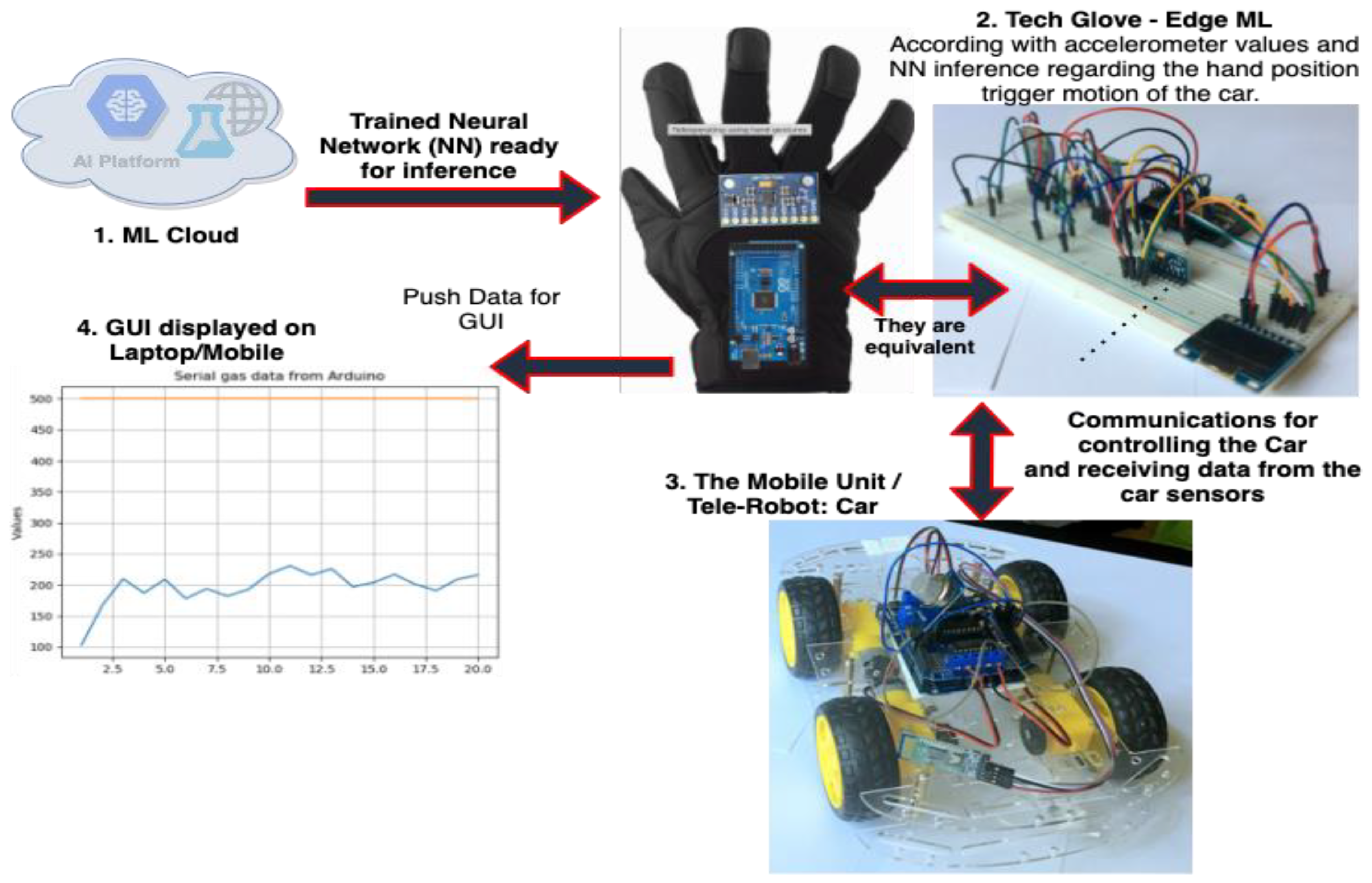
The proposed proof of concept (PoC) solution is a teleoperated robotic unit that can detect a variety of gases with the potential to become dangerous if they exceed the accepted limit, such as alcohol, CO, CO₂, and methane. It consists of four main elements:

▪

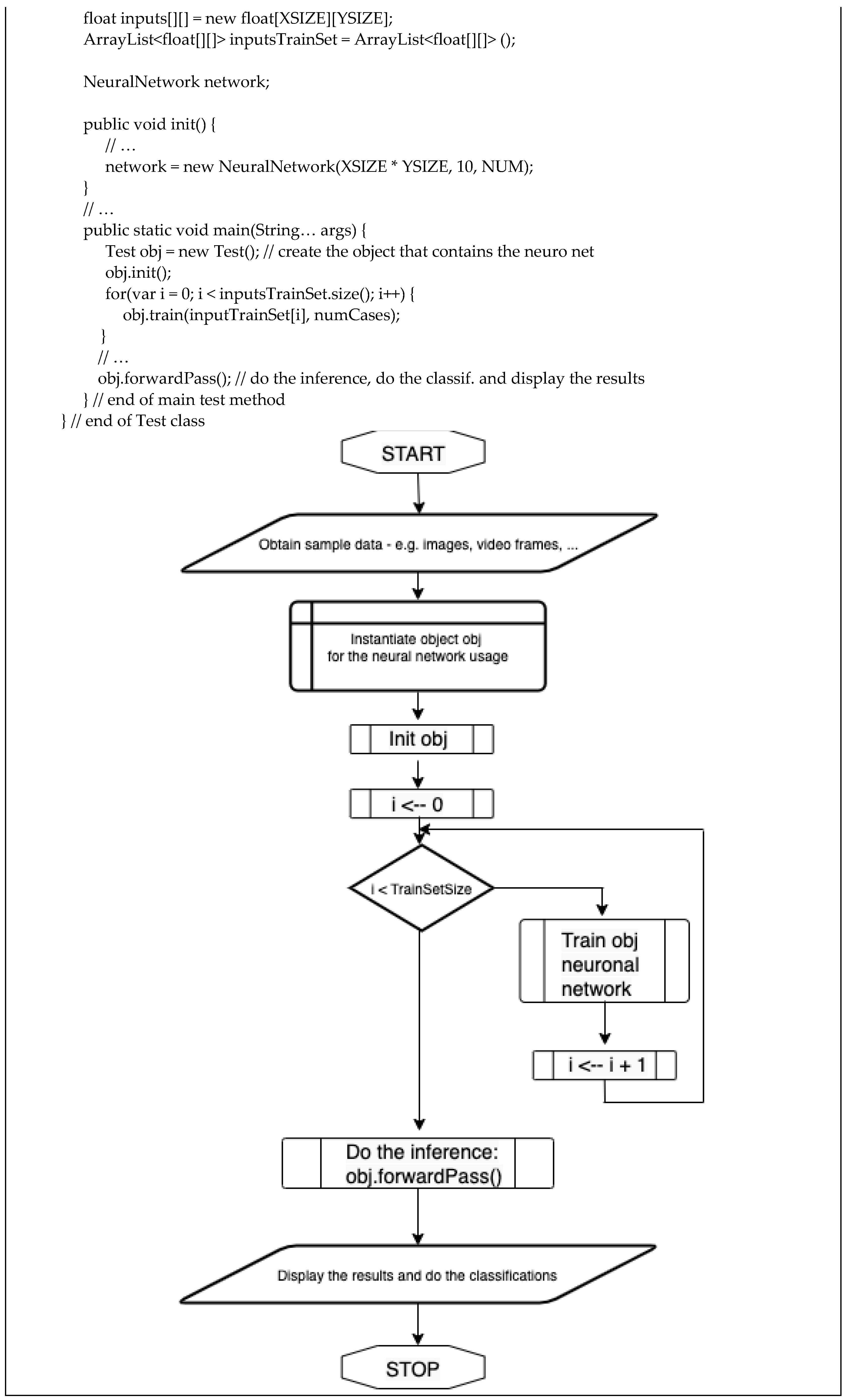
Machine Learning Cloud: It is used for training the neural network to improve the movement decision of the telerobot ordered by the tech glove according to the hand’s positions.

▪

Tech Glove: It is a glove that has attached an IoT smart device. The IoT smart device has a gyroscope sensor, Bluetooth modules, and a display. It communicates with the robotic car via Bluetooth and sends information about the direction in which the robot should move and receive gas data. For the tech glove, it is sufficient to have the values from the gyroscope and accelerometer, but with the use of the neural network inference, the control is more refined.

▪

Mobile unit/(Tele)Robot: This is a car robot that moves and detects gas sources by reading and interpreting atmospheric data. It has attached a gas sensor that detects gas leaks and sends it via a Bluetooth connection to the controller.

▪

User interface: the user interface is the graph generated by the data received from the car. It establishes a Bluetooth connection with the robotic glove and generates real-time graphs that plot the data. In addition, it receives a live-streaming video from the robotic car to visualize the environment.

In this way, the operator can guide the robotic unit to gather valuable gas data when human health is in danger. Gas leaks can be prevented in a secure manner, and users can visualize data in an interactive manner. Figure 5 presents the components of the PoC.

The tech glove wiring schema is detailed in Figure 6 and

Table 2. The Tech-Glove PIN Schema.

Component	Component PIN	Arduino PIN
PC HC-05 Bluetooth	VCC	5 V
	GND	GND
	TXD	D10
	RXD	D11, GND
Master HC-05 Bluetooth	VCC	5 V
	GND	GND
	TXD	D4
	RXD	D5, GND
MPU6050	VCC	5 V
	GND	GND
	SDA	A4
	SCL	A5

and

Table 3. The Tech-Glove PIN Schema for the Display.

Component	Component PIN	Arduino PIN
OLED Display	VCC	5 V
	GND	GND
	D0	D13
	D1	D9
	RES	D8
	CS	D7
	DC	D6
	VCC	5 V

:

In terms of hardware for both the tech glove and the tele-robot car, one distinguishes a variety of elements that are used to build up the robots. Hardware includes Arduino UNO and Nano, two HC-05 Bluetooth modules, an MPU6050 gyroscope, MQ-2 gas sensor, an L293D motor driver shield, motors, wheels, chassis, and peripherals.

Arduino UNO is the most popular microcontroller board used in robotics PoC (not production ones). It has a large support community owing to its applicability. It is easy to comprehend, and it can be easily incorporated with other components, such as LEDs, sensors, or other development boards.

Arduino is an open-source platform that facilitates access to code written by other electronic enthusiasts. Projects available online differ in difficulty and capture all ideas of the community.

The Arduino UNO board is equipped with a power jack, reset button, 16 MHz resonator, 20 digital input/output pins, and an ICSP header. It is affordable and easy to replace when required. There are a variety of ‘shields’ that can be attached to the Arduino board to add more functionalities.

Arduino Nano is a smaller version of the Arduino UNO. It incorporates almost the same functionalities and can be easily integrated into a circuit. It has 14 digital pins and 8 analog inputs, supports I2C communication, an AREF pin for voltage reference, and a Reset pin used for adding a button to block the circuit. The board communicates via UART serial communication available on TX (1) and RX (2) digital pins and can be easily programmed via Arduino IDE.

Bluetooth module HC-05 is used for long-distance communication. It consumes low energy, and its small size makes it easy to incorporate in various projects. It has a signal radius of 10 m and can be used in robot-laptop communications or robot–robot communications. It can be configured in two modes: slave (pin value 0) and master (pin value 1). These are some common commands used to set up the modules.

▪

AT—verifies the connectivity to the module.

▪

AT+ROLE?—checks the role of the Bluetooth module; it returns 0 if it is in the slave configuration and 1 if it is in the master configuration.

▪

AT+RESET—resets the module configurations.

▪

AT+PSWD=—changes the password of the module. Note that the default password is ‘1234′; it is required for pairing the devices.

▪

AT+ADDR—returns the address of the module; it is also required for pairing the devices.

MPU6050 unit is a device equipped with a 3-axis accelerometer, 3-axis gyroscope and a digital motion processor that reads the orientation in a 3-dimensional space. It is used to detect the motion and orientation of the objects. It has three analog-to-digital pins used to convert to digital gyroscope outputs and three analog-to-digital pins that convert to digital accelerometer outputs. MPU6050 is small, flexible, and provides fast gesture conversion.

MQ-2 gas sensor was used to detect combustible gas leaks. The sensitivity of the sensor can be adjusted by a potentiometer, and it is fast responsive to gases such as H2, liquefied petroleum gas (LPG), methane (CH4), carbon monoxide (CO or smoke), alcohol (C2H5OH or ethanol), and propane (C3H8). It is a very fragile component, so there is a list of items that should be avoided when working with the MQ-2 gas sensor:

▪

Long-time storage without electrification should be avoided because it produces a reversible drift.

▪

It should not be exposed for long periods of time to high gas concentration environments because it may affect the sensor characteristics.

▪

Water condensation can affect the sensor performance.

▪

Concussion and vibrations should be avoided, as they may lead to hardware damage or down-lead responses.

L293D Motor Driver Shield is an integrated circuit that amplifies the low input current and provides a higher-current signal to the motors. It is a shield compatible with Arduino UNO, which can be easily attached to improve performance. Using this shield, different types of motors can be assembled to create a movable robotic unit. We can control four DC bi-directional motors with speed ranging from to 0–255, two stepper motors, or two servo motors at a time. The motor driver shield can be powered in three ways:

▪

Ensure a single DC power supply to the Arduino board, which supplies power to the shield.

▪

Two different DC power supplies, by plugging one of them into the DC power jack of the Arduino and one into the EXT_PWR block attached to the shield.

▪

A USB that provides power to the Arduino board and a DC power supply connected to the EXT_PWR block of the motor shield (recommended method).

Note: When supplying power to the EXT_PWR block, the power supply jumper must be removed. Otherwise, it may damage the shield and the Arduino.

OLED Display 128 × 64 SPI or I2C—this display module is small and compact, which makes it perfect for displaying small amounts of data (e.g., smart watches). It can display 128 × 64 points and consumes a low amount of power when it is used at full capacity. It can communicate with microcontrollers via a serial peripheral interface or inter-integrated circuit protocols.

In this project, it is used to display meaningful information and messages on the robotic glove, such as messages that let the user know whether the robots are connected via Bluetooth, or whether the robotic glove is powered on, the battery level, etc.

4.1. Motors, Wheels, and Chassis

The robot vehicle is equipped with four DC motors and wheels that allow movement on the terrain. DC motors convert direct current electrical energy into mechanical energy. The speed can be easily adjusted, and these motors are mostly used in toys and appliances. The four motors used in this project come together with a distinctive wheel that can be attached. All hardware used for the mobile robotic unit was mounted on a car chassis.

4.2. Peripherals

Peripheral components include jumper wires, soldering iron, 1 mm solder, four 9 V batteries, two 9 V battery connectors, breadboards for development, pin headers, buttons, and resistors. These peripherals connect the hardware components and provide a power supply to the robotic units.

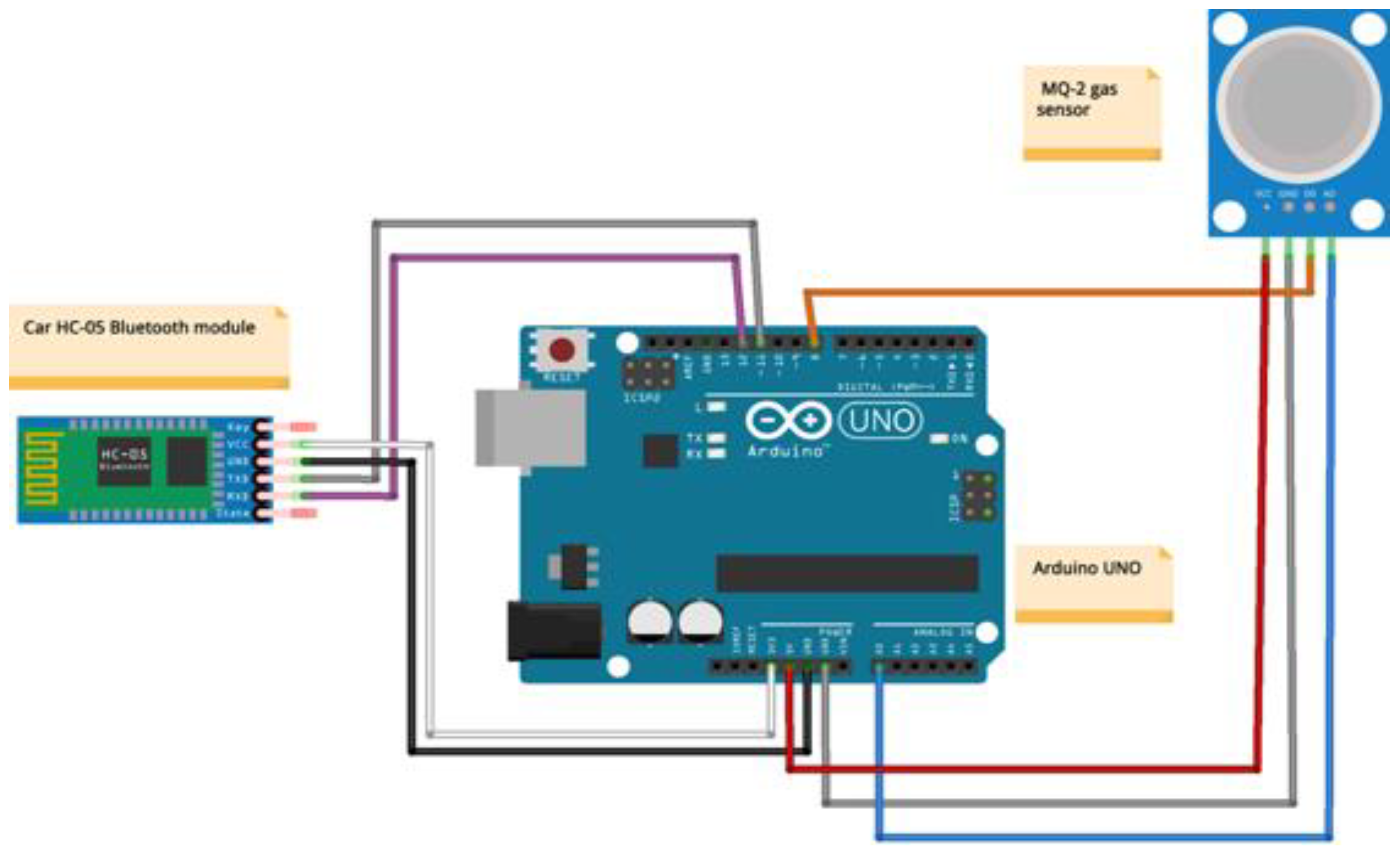
Figure 7 and

Table 4. The Car PIN Schema.

Component	Component PIN	Arduino PIN
Car HC-05 Bluetooth	VCC	3 V
	GND	GND
	TXD	D11
	RXD	D12
MQ-2 Gas Sensor	VCC	5 V
	GND	GND
	D0	D8
	AD	A0

show the tele-robot/mobile unit/car hardware wiring schema.

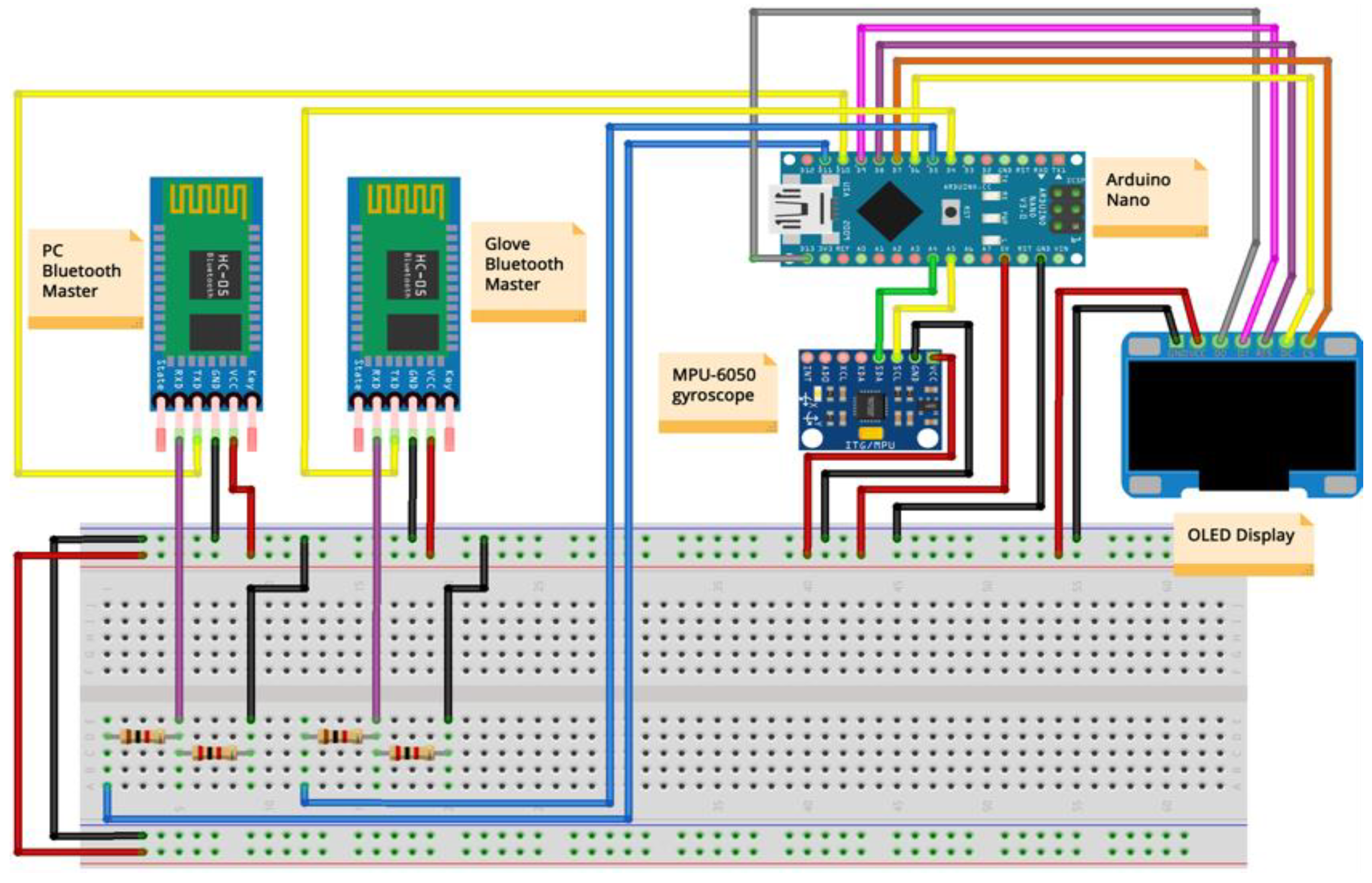
The project involves two major parts: the robotic parts and the GUI plot generation. All these parts communicate via Bluetooth serial communication. Glove has two Bluetooth modules incorporated, one for linking with the robotic car and one for binding to the PC’s Bluetooth.

The glove has attached the MPU6050 gyroscope sensor, which is used to analyse the tilt and position of the hand. The starting position of the teleoperation begins with the hand relaxed, parallel to the ground, with the first open palm parallel to the ground and the inside of the hand oriented to the ground. MPU6050 reads the data and converges it into an XYZ-axis table. The X axes read whether the hand is in a parallel position with the hand raised or lowered in place from the fingers. The Y axes read whether the hand was in a horizontal position relative to the ground and was slightly rotated to either the left or right. The Z axes read the rotation of the whole hand when it has a palm parallel to the ground.

These XYZ values were tested for specific intervals, interpreted as movements. Therefore, we can distinguish five types of movement as presented in

Table 5. Movement Code Mapping.

Movement	Code	X	Y	Z
START -middle-	1	[20, 90]	[300, 360] or [0, 60]	[70, 100]
SPIN Right	2	[340, 360] or [0, 20)	[20, 90]	insignificant
STOP -middle-	3	[340, 360] or [0, 20)	[340, 360] or [0, 20)	insignificant
SPIN LEFT	4	[340, 360] or [0, 20)	[270, 340)	insignificant
BACK -middle-	5	[270, 340)	[340, 360] or [0, 40]	(260, 280]
-undefined-	0	-	-	-

.

For the SPIN and STOP movements, the Z-axis is insignificant because it depends only on the tilt of the hand to the right or to the left (Y-axis). For the START and BACK methods, the Z-axis is significant because once the fingers are lowered or raised to incline the hand up or down, you cannot rotate it to the left or right. This must be in a steady position.

For undefined or faulty data, glove sends 0 to the robotic car, which has the same effect as the STOP method.

Glove sends the code that is processed by the robotic car into movements. This car has four DC motors attached, which can be activated and deactivated, and set to a speed with values in the interval [0, 255] (0 is for STOP and 255 for full speed). Clockwise from the front left of the car, the motors are denoted as 1, 2, 3, and 4 to quickly identify which one must be activated or deactivated. For example, in a SPIN left motion, the left motors (1 and 4) run backward while the right motors (2 and 3) run forward, causing the car to spin in place.

Once the robot Car can be remotely controlled, it can read and send data back to the glove. The MQ-2 gas sensor attached to the car reads and converts the voltage values into meaningful data and sends these values back to the glove via Bluetooth. It has also attached a mobile phone connected to the same Wi-Fi as the PC unit that streams live and records the car’s environment. Teleoperation would be blind without video streaming, which makes Wi-Fi connections a functional and important element in the project. Without establishing a secure and strong Wi-Fi signal, the operator has no visual feedback from the surroundings.

The converted gas values are received by the glove and passed to the PC via a separate serial Bluetooth communication. The PC unit connects to the HC-05 Bluetooth module, and the GUI module establishes a connection to this port. It constantly receives gas data values that are stored in an array based on the FIFO principle. The programme will constantly plot the new array of elements that create the effect of an endless line signifying the gas level at a certain moment of time.

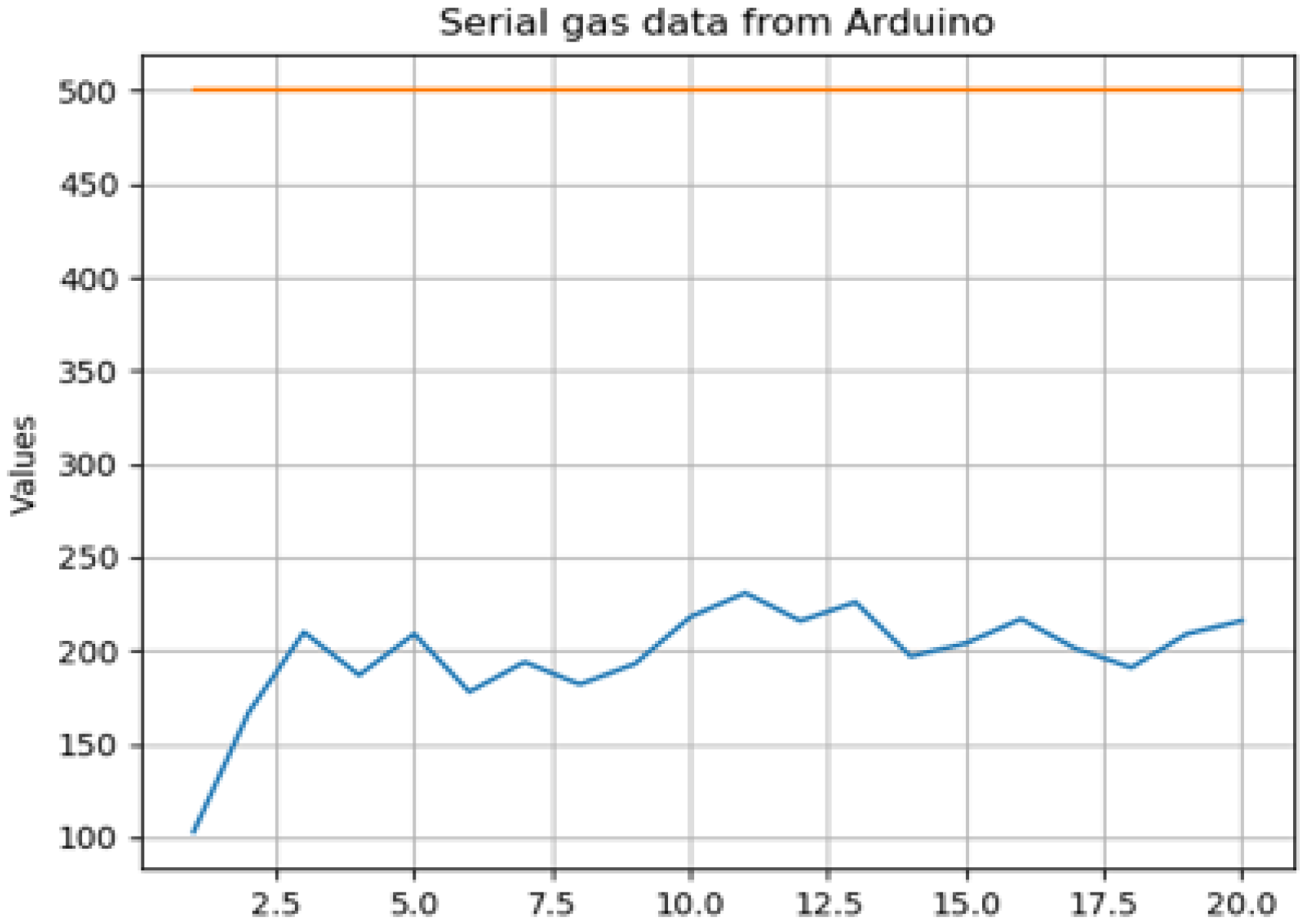
To test this system, the level of security must be established. Compounds such as CO and CO₂ are difficult to simulate at dangerous levels under safe conditions. As a result, acetone is considered an inflammable substance used to test the robot.

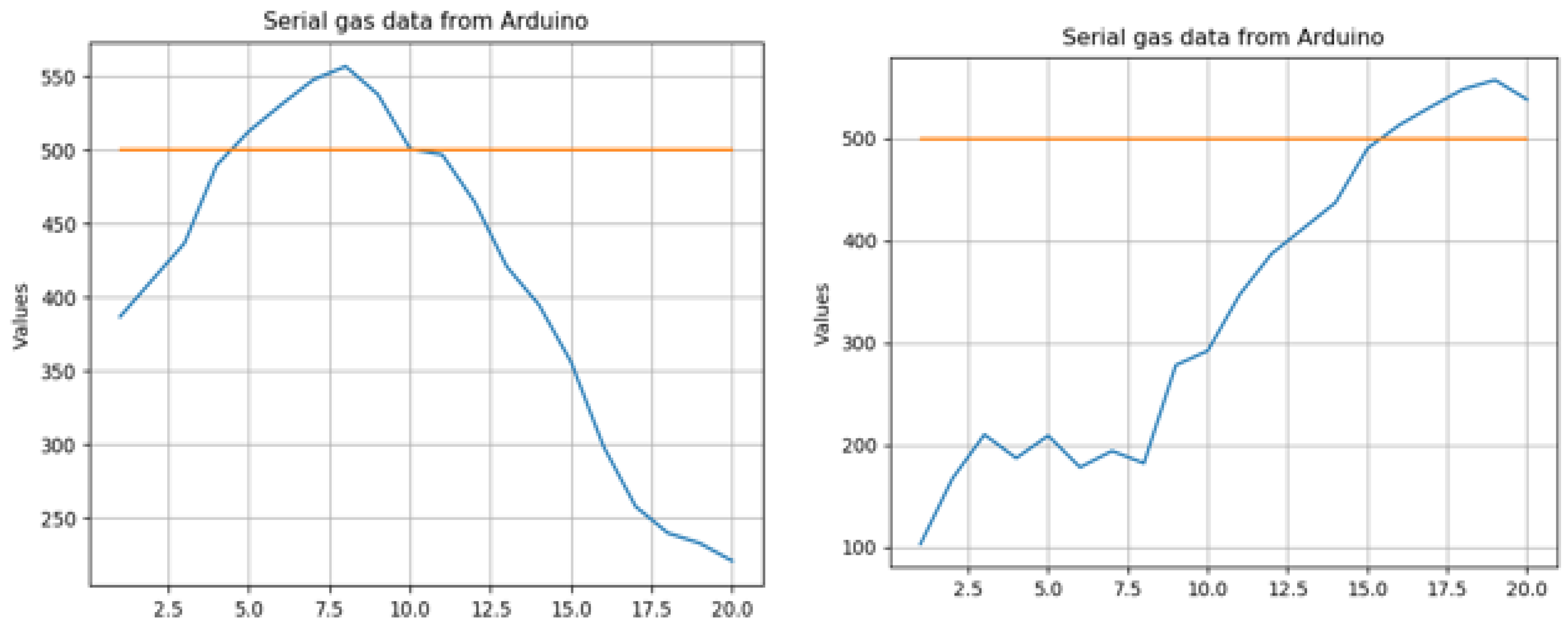
The graph in Figure 8 shows a normal acetone gas curve with all values below 250 ppm. This level is safe and does not cause harm to human health. An orange line was drawn to display the accepted limit of moderate acetone ppm levels. To test the system, a cloth was soaked in acetone and left on the floor. When the robot car passed by it at a close distance, MQ-2 sensed the vapours and spiked above a 500-ppm level threshold for a short period of time, Figure 9.

The

Table 6. The complexity overview for the autonomous robot vehicle architecture.

Features	Details
I/O Comms	IN: glove commands based on real time video stream of environment
	OUT: plot data graph that show the levels of different dangerous gas products
Running time	Average process time at around 15 frames/second
Efficiency	Improved car handling with an ML inference model on the car robot
Code complexity	Complexity between O(n) and O(n^2)

gives a good understanding about the complexity of the entire solution from a different point of view.

The Edge ML can be used for the video stream feed as well, but we preferred to use it to enhance the reported values of the accelerometer from the tech glove and to do inference on the module from the glove. This allowed better refined values after the feed-forward neural network was applied, as presented in the second section of this paper.

5. Visual Computing of the UAV/Drone PoC Development, Experiments and Results

The aim of this section is to present how machine learning and drones can be used to facilitate the control of an unmanned aerial vehicle through poses and gestures made by an individual, as opposed to the classical usage of remote controllers, smartphones, or other devices. To achieve this goal, the authors used a Raspberry Pi 4 Model B/4 GB and an MPU6050 6-DoF accelerometer and gyroscope to control a DJI Tello drone through hand movements and gestures. This topic is like the previous section of this paper; however, in addition to hand movements, pose estimation algorithms are used to recognize and classify the positions of multiple individuals’ bodies from the drone’s video feed.

One of the most interesting branches of deep learning is computer vision, in which convolutional neural networks (CNNs) are the most applied in practice. This allowed impressive feats of engineering, such as advances in autonomous vehicles through autopilot, autonomous anomaly detection in production lines, and cancer diagnosis through radiographies [60]. Computer vision also helped in landing the NASA Perseverance Mars mission by analyzing the planet’s surface in real time and detecting the best place for landing.

The most common applications of computer vision are posed estimation, optical character recognition, facial recognition, gesture recognition, pattern recognition, and object recognition. Current usage is seen in classification problems, a subset of supervised learning. This is because of the reliability of the detection of the edges from images. Stacking detections on top of each other makes it easier to “recognize” the desired feature in an image. Furthermore, because videos are nothing but thousands of image frames that are changing rapidly, the same approaches have high performance for the videos as well.

A typical workflow of a Computer Vision solution could be structured as follows:

▪

The first stage involves image acquisition. The most important characteristic of an image is its illumination. Closely following in importance, in no particular order, comes the camera quality, contrast, and focus [66].

▪

After acquisition, most images are pre-processed before any other work is done to make it easier for a model to extract features from this input. Pre-processing can be as easy as size reduction or as complex as hue, saturation, and gamma corrections. Often, these two steps can lead to either a successful model or an ever-failing model.

▪

Feature extraction is the next step in a typical computer vision pipeline. Usually, this refers to the detection of lines, edges, ridges, corners, etc., which remain the sole components of the processed image, by reducing all to a background. After extracting the relevant features, the pipeline then detects and segments the data into regions or sets, which contain the most important information for finding the optimal solution to the problem. These are the prerequisites needed to finally reach the crucial step in a pipeline that handles high-level processing. It validates the input data and estimates parameters, such as position, distance, and size.

▪

High-level processing is a step in which recognition or registration is performed [66].

▪

The final step in a typical computer vision pipeline is the decision-making step. For example, in classification problems, this step aims to determine whether the input data is a match. For sensitive solutions, such as those from the medical field, this step depends on the notification of an approval performed by a human [66].

It is not mandatory for all models to follow this structure; however, sometimes, the input data is in a format that allows for some steps to be skipped. The same step needs to be replicated at different points through the pipeline lifecycle. There are cases in which only using image processing is sufficient to obtain the solution. The effect stemming from the varied approaches to any single problem is prevalent in machine learning, not just computer vision. This is because most of the time, the best model is the one tailored to the input, rather than the one recommended by theory alone.

Keypoint detection, commonly referred to as pose estimation, is a superset of models used to detect and estimate the pose of one or more humans in images or videos. It can also be extended to the pose of other living beings, such as mammals or reptiles. Common approaches to this problem are models, such as convolutional pose machines or part affinity fields. They are commonly used in articulated body pose estimation, a set of algorithms concerned with recovering articulated body poses by using joints and rigid parts Ref. [67].

The relatively recent lack of efficient, reliable, and scalable real-time estimation of two-dimensional body poses is a longstanding problem that allows machines to gain a more meaningful comprehension of people in images and videos [68]. Some algorithms provided high accuracy at the expense of performance and hardware requirements, while others that mitigated those issues suffered from performance drops proportional to the increase in people in the input data.

Convolutional pose machines aim to resolve these problems by combining the benefits of both pose machines and convolutional architectures. Using convolution to extract features of the image and the spatial context directly from data, they used the sequential learning process of associating multi-part cues and the overarching image. Using multiple convolutional networks, each iteration diminishes ambiguity from the initial detection, reducing the final prediction to the relevant key points. This approach allows for end-to-end training through backward propagation, with predictions benefiting from spatial models that are dependent on the input image [67].

Pair Affinity Fields is a term coined by the team of Zhe Cao et al. of Carnegie Mellon University’s Robotics Institute, whose members and works are presented in [68] in more detail. It refers to a non-parametric representation of body parts that are associated with an individual. The representation is created through two-dimensional vector fields, where the position and direction of the body parts are encoded. This allows for more meaningful insight into the anatomy of a person’s body pose [68].

Owing to the large number of algorithms, frameworks, and models that exist in this scientific study, this study focuses on what is currently considered the state-of-the-art model for key point detection. This model was developed by Zhe Cao, Gines Hidalgo, Tomas Simon, Shih-En Wei, and Yaser Sheikh of Carnegie Mellon University’s Robot Perception Lab from Pittsburgh, Pennsylvania. It is a model used to estimate 2D poses of multiple people in real time, including hands, feet, and faces, using partial affinity fields. Their model is considered in such a high regard that it is now included in multiple machine learning frameworks, such as Google’s TensorFlow or OpenCV’s Deep Neural Network module.

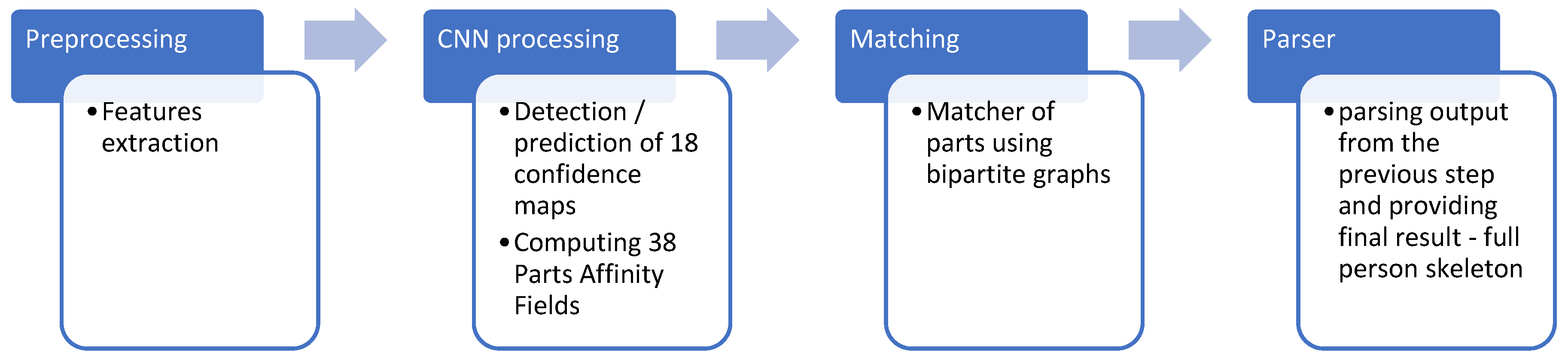
The architecture used by OpenPose comprises a pipeline with four steps. The first is tasked with receiving an input image. The second step has two sub-steps, which ran in parallel, one handling the detection and prediction of confidence maps, while the other handles the part affinity fields. The output is then processed by the next pipeline component, which runs a bipartitely matching the two results, creating the initial estimation result, which is then fed in the last step, which parses the result and provides the final estimation, Figure 10.

The convolution employs a 3 × 3 kernel for each iteration in a 10-layer neural network. OpenPose supports hand and facial estimation and fully predicts the anatomy of the people in the input image(s) [68].

The approach proposed and employed by [68] provides great performance and efficiency, as it focuses on all the subjects in the input at once, and uses a bottom-up approach, first predicting body parts and associating them with everyone. After generating the part affinity fields, each iteration infers who owns each body part, reducing the time needed to estimate by half.

The primary hardware component of the solution was a drone. The DJI Tello drone model was used because of its availability to regular consumers, size and weight (which allows for no regulatory approval from the government for its usage), and affordable price. It benefits from an easy-to-use API, developed, provided, and documented by the DJI. To communicate, it broadcasts a Wi-Fi UDP connection that is accessible to any controller. The term controller represents any programme that sends commands to the drone. The architecture is composed of three layers: the command layer, the state layer, and the video stream layer, each using a different UDP server and port and accepting clear text commands/requests.

The second part of the architecture is composed of two separate hardware devices. The first is a Raspberry Pi 4 Model B/4 GB single-board computer. The other is an TDK InvenSense MPU6050 6-DoF (degrees of freedom) accelerometer and gyroscope: Invensense Manufacturer, USA. These components are connected through an HQ breadboard of 830 points using male-female-colored wire connectors. To see the live drone feed, the Raspberry Pi is connected through a USB-C cable to an Android device supporting USB tethering. The phone is then used to access the single-board computer through the VNC protocol, using the VNC Viewer client made by RealVNC. The Raspberry Pi hosts and runs a VNC server. In production, the Raspberry Pi single-board ARM computer is not recommended, but for the PoC is good enough, owing to its availability, price, and choice of embedded Linux operating system.

The MPU6050 addition was made because of its well-established accelerometer and gyroscope, having a technical sheet that is intuitive and has a low power consumption of 3.3–5 V.

The cables connecting the Raspberry Pi and MPU6050 are male-female-coloured wire connectors, which have a length of 20 cm. While the MPU6050 supports running on 3.3 V power, it is possible to use the standard 5 V power GPIO connector of the Raspberry Pi because no additional electronic components will be connected to the single-board computer, thus having no competing hardware “modules” to distribute electric current to. Owing to safety concerns, for most of the development, the accelerometer was rested on the breadboard to ensure that no conducting surfaces would touch it and to make it easier to handle, while analyzing the received data.

The approach of using the poses of the person facing the drone to control its flight showed its limitations early in the development process. Since the protocol used by the drone to communicate was UDP, this already meant that the video stream it was sending was unreliable. This means unreliable estimations of a person’s positions. In this situation, the control would either be sparse or wrong, and the computer vision algorithms have a high probability of running into difficulties predicting positions. Because of these concerns, the approach has been changed to employ both gesture interpretation using the accelerometer and gyroscope and pose recognition on the video stream. The major change from the initial idea was the computer vision component. Instead of using this feed to decide the path that the drone would take, it now detects the bodies and poses of people in front of the drone and displays it to the “pilot,” on a GUI.

Owing to these changes, the control drastically increased in reliability because the MPU6050 is connected directly to the Raspberry Pi, meaning little input lag and no data loss. Reliability also increases with longer travel distances from the person controlling the drone, allowing them to access any area within the drone’s maximum flight distance. Currently, drones are capable of surveying different areas, even those inaccessible to humans. This brings much more utility to the solution, as it can be used to find missing or trapped people, scout areas ahead of the person reaching them, or even provide cues to help position it in better suited places for different purposes, such as cinematography. Because the computer vision pipeline works even in above-normal bright or dim environments, it can still be used, even if human eyes are not able to properly identify the surroundings of the drone.

In terms of architecture, as mentioned above, there are several constraints that should be known, which influence the development and architecture of the PoC. First, the biggest constraint is the UDP protocol used by the drone to communicate. Because this is an unreliable connection, the video stream cannot be used as the sole method for piloting the drone because the computer vision pipeline would not be able to constantly determine the correct commands to send to the drone. This would not only be undesirable but also dangerous, as the drone would fly without control for varying periods of time.

The second constraint is the performance impact of the solution. Because it uses threads, networking, I2C, and a machine learning pipeline, the hardware required to run the programme needs to be sufficiently performant. This limited the options, leading to the choice of the Raspberry Pi 4 Model B/4 GB. While less performant single-board computers can handle the load, it is normal to ensure the best performance availability even for a PoC.

Another constraint comes from using the Raspberry Pi, along with the breadboard and short-length cable connectors. Because flexibility is important in prototyping the design, these components are needed. This means that the final product is not wearable because the wires are not soldered onto the breadboard, single-board computer, or MPU6050 MEMS. Without soldering, it is easy to accidentally unpin them, losing power, or connecting components. As the Raspberry Pi has a moderately high-power consumption, needing to be kept plugged into an electrical socket, this would also hinder wearing the device on one’s hand.

The orientation of the MEMS header pins creates another constraint, as they define the position and orientation of the gyroscope and accelerometer. This determines the logic for gesture detection, as it depends on which axis is placed parallel to the body and which one is placed perpendicularly, as well as on which plane, they are found. This limits the possible ways to wear the MPU6050, as well as how gestures are performed by the “pilot.” In addition, the header pin orientation also determines how the Raspberry Pi is positioned with respect to the MEMS. We decided to solder the MEMS header pins using a 90-degree pin connector, which allowed the MPU6050 to rest horizontally on a hand, parallel to it. We find this to be the most natural option. This meant that, from the perspective of the “pilot,” left and right are directions found on the Y axis, left being a positive value, right being a negative one, while forward and backward would be found on the X axis, with a negative value meaning forward and a positive one meaning backward. Up and down are found on the Z axis, with the natural expected directions, up meaning a positive value and down a negative value.

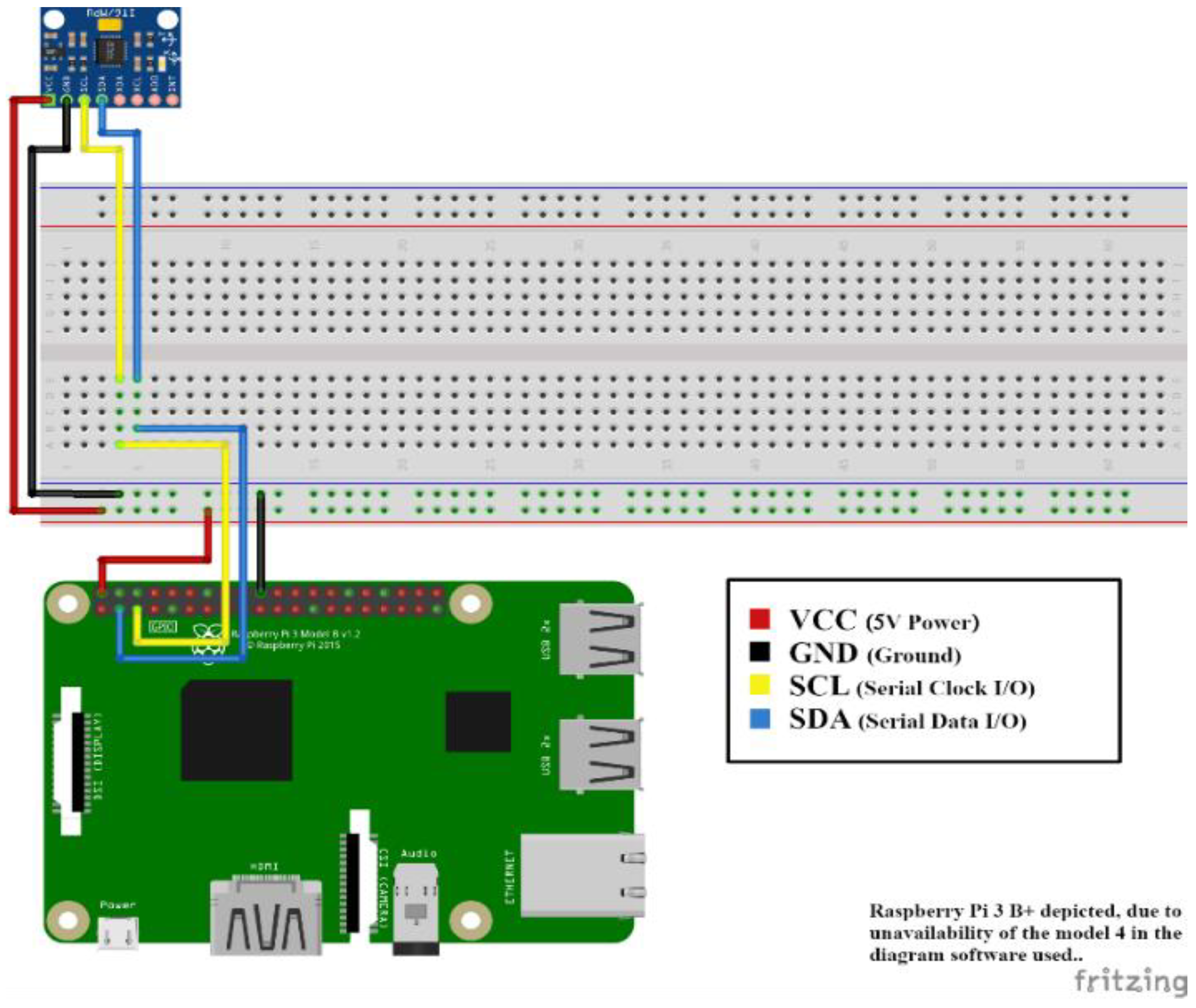
The following workflow is required to start the solution. First, the Raspberry Pi and the MPU6050 need to be connected, as shown in Figure 11, through male-female wire connectors placed on the breadboard. The Raspberry Pi needs to be powered on and, after a short wait, the Android smartphone used as a screen can connect to it, using the VNC protocol. There are several ways to obtain the IP of a single-board computer. Because Android no longer supports static IP addresses for USB tethering, the configured Raspberry Pi was connected to the same Wi-Fi network router where the mobile phone was connected. This allows the use of a static IP for this network. The configured Raspberry Pi uses the 192.168.1.71 IP v4 address, thus allowing the connection from the Android device via SSH. Finally, after connecting via SSH, one can obtain the USB tethering dynamic IP address and connect via the VNC Viewer client made by RealVNC.

The next step is to power the DJI Tello drone and connect it to its Wi-Fi network, using a smartphone to control the Raspberry Pi. Finally, the solution can start from a terminal. Once it is running, the device file is first opened, and the bus address of the MPU6050 is configured. Subsequently, the program calibrates the MEMS by reading the accelerometer and gyroscope data for several iterations and averaging it to compute the initial offset. The process and progress are shown in the terminal via standard output. After calibration, the terminal shows both the MPU6050 data and communication with the drone, such as what commands are sent, and the received responses. In addition, a GUI also starts to display the video stream of the drone, overlaid by the pose estimation resulting from the computer vision pipeline.

To fly the drone, a take-off command must be issued. This is performed via a special gesture recorded by the MPU6050. This gesture is unique to the previously mentioned command, and unless the drone is landed once more, it will not have any effect. To land the drone, a special secondary gesture is required. Both gestures were made on the Z-axis of the accelerometer. Flight is controlled via natural hand movements and gestures, such as raising the hand, leading to increasing altitude, lowering it leads to downward movement. Left and right flights are performed in a similar manner by rotating the hand on the X-axis of the gyroscope. The orientation of the drone is controlled by rotation of the hand on the Y-axis of the gyroscope.

To recognize a pose and display it on top of the raw video stream of the drone, a specialized service is created. To assign the drone live feed and use it in the recognition, the service exposes a setter method. Start and stop methods are also exposed to begin and end the process of displaying the graphical user interface, which will show the output of the machine learning pipeline. Because the process is generally slow, especially when the number of people for a given frame is large, and because the Raspberry Pi does not have a dedicated GPU or many resources and processing power, the entire recognition and display process is running on its dedicated thread, to allow the drone to be continuously controlled in real time through the movements of the accelerometer and gyroscope of the MPU6050.

To improve the performance of the pose recognition model, it uses only the general body model. OpenPose provides multiple specialized modules to create an accurate representation of the human body. These include complete facial recognition and complete hand and foot recognition models. However, to use these models, considerable computational power is required, and a dedicated GPU is recommended. Considering these issues, along with the technical specifications of the Raspberry Pi, it would be unrealistic to expect a complete human body model to be identified using this hardware. Because no significant benefits will result, based on the main applications of this solution, and because of the drawbacks, only the general outline of a body is presented.

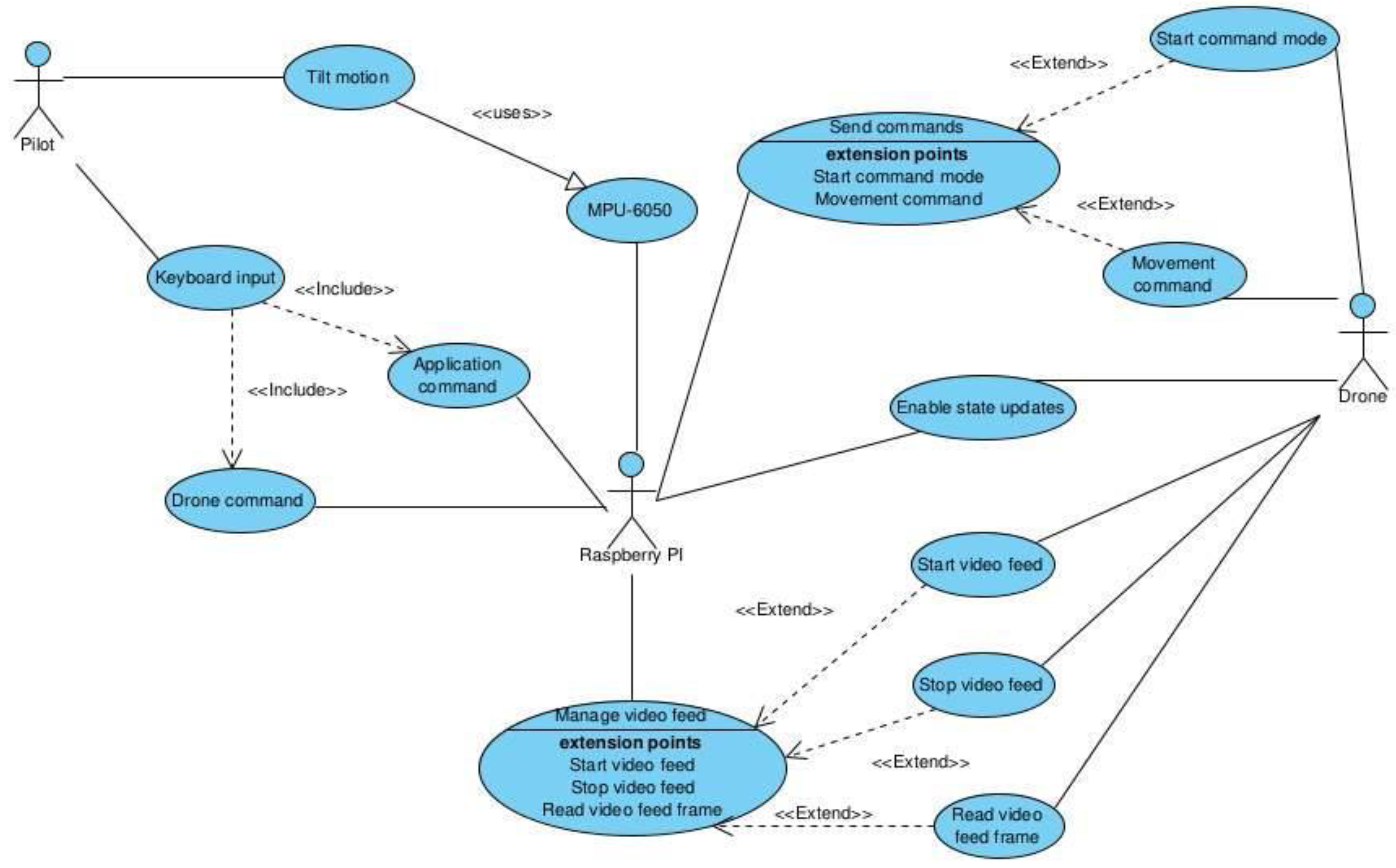
In terms of development, Figure 12 shows the general UML use case diagram for the solution proposed in this study. The three main actors are the “pilot,” the Raspberry PI, and the drone.

The MPU6050 should not be classified as an actor, as it has no function on its own, only when paired with a single-board computer. Thus, it is used by the tilt motions and the Raspberry PI but cannot be identified as an independent actor. The pilot can make tilt motions, as described previously, or input direct commands through the keyboard to compensate for the reduced number of gestures available. The direct commands are of two types: the application commands, such as quitting the application and the drone commands, preceded by “c”, which are sent directly to the drone. The Raspberry PI, having those two inputs, manages sending commands, such as starting the command mode or movement commands, enables the state updates available from the drone and manages the video feed, by starting or stopping it and reading frames of the live stream. Finally, the drone executes each input received from the Raspberry PI and sends responses as detailed in its specific developer SDK manual.

The software components tasked with the behaviour are structured into multiple classes, interfaces, and Data Transfer Objects, such as AccelerometerData and GyroscopeData. The structure closely follows SOLID design principles and clean code practices. The MPU6050 class, for example, uses an I2C communication service that handles low-level information exchange between the Pi and the MEMS. This service is a member of a class and, following the dependency inversion principle, it is kept as a reference to an interface, decoupling implementation from usage. Configuration options for the MPU6050 are also provided via an options DTO, which has default values for all the required register addresses and system configurations, such as accelerometer and gyroscope ranges (both of which are further structured as individual DTOs). The default values are stored as public static members of an inner class.

The I2C service interface exposes only a few methods, the minimum required to communicate through this protocol. Specifically, the interface allows reading and writing byte data from and to a register address. The implementation of the interface uses its constructor to connect to the bus address of a device. This is done by providing the device number and bus address (as a hexadecimal value). If either operation fails, the respective custom exceptions are discarded. Continuing the topic of communication services, UDP communications are handled through a helper class, with static methods for socket API programming. Since the sockets API is a C API, it means that all calls are stateless; thus, we found no compelling argument to create a more advanced pattern. As with the previously mentioned service, the UDP helper methods throw custom exceptions in the case of failure. All exceptions that are thrown by the solution are custom exceptions, which inherit the runtime_exception base class available in the standard C++ library.

DTOs in the solution do not follow the strict rule of having only public members because of the extensibility of the C++ operators. To make code easier to follow and less verbose, all the DTOs have at least a couple of operators overloaded. For example, AccelerometerData and GyroscopeData DTOs have overloads for arithmetic operations, which are needed to process the respective sensor’s data to provide meaningful output. The arithmetic operations, which are referred to as division, addition, multiplication, or subtraction of values, and other DTO instances.

This allows clean, short, and easy approaches to understand, change, and debug operations.

To benefit from polymorphism, there is a usage of another recommended approach, employing smart pointers, throughout the C++ code. This is preferred to the classical C-like memory handling because the smart-pointers handle allocation and deallocation based on scopes and object lifetimes, following the RAII principle (Resource Allocation Is Initialization). Using a combination of unique pointers (which allow for only one reference to a single heap-allocated object) and shared pointers (allowing for multiple reference to the same heap-allocated object), this ensured that no memory leaks would occur and remove the memory management responsibilities from development. With the use of move semantics, one can pass ownership of a unique pointer, such as when providing an I2C service to the MPU6050 class, without violating the smart-pointer principles.

Because C++ is structured in header and source files, this leads to many files that need to be linked and compiled. Adding to the complexity, many compiler arguments are usually required for generating warnings and errors and for optimization, as well as libraries that need linking. For a complex project such as the one that is the subject of this chapter, this process is troublesome and highly verbose. To mitigate these issues, the best practice agreed in the industry is to use build systems. The most popular is the Make or CMake build system, which handles cross-platform, cross-architecture, and multiple compilers building of solutions. It can also handle the packaging and testing of solutions.

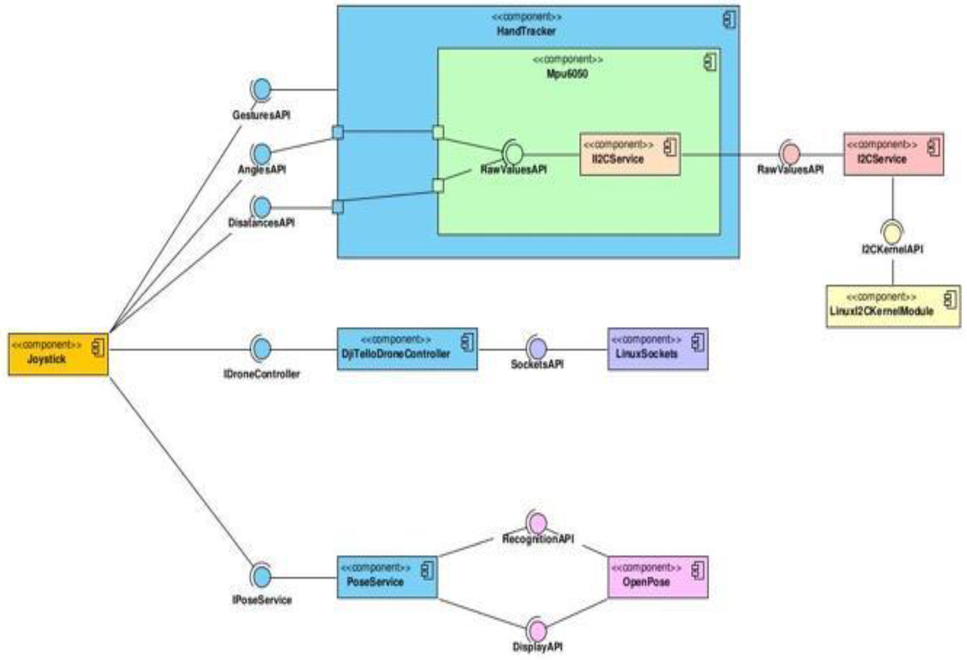
The diagram in Figure 13 describes the general components of the solution. Not presented in it, is the subsystem used for the creation of drone controllers, as it is not tied directly into the joystick or main solution, as controllers can be instantiated without the factory mechanism available. As discussed above, is the entry point of the solution, that is, the Joystick component. It is dependent on three others: the PoseService, the DjiTelloDroneController, generally any drone controller supported, and the HandTracker.

The dependency on the PoseService is done through the IPoseService interface, which exposes the API required to recognise the bodies that exist in the video stream. Furthermore, this component is dependent on the underlying OpenPose library, using its recognition and frame-display APIs. The drone controller dependency is accomplished through the IDroneController interface, which exposes the APIs for sending commands, receiving responses, and state of the drone, as well as retrieving its video stream. In addition, this component uses the Linux sockets API to manage the sockets created for UDP communications with the drone. The final main component that the Joystick uses, the HandTracker, fulfils its dependent state through gestures, angles, and distances APIs. In addition, the MPU6050 component is responsible for obtaining and processing the values from the MPU6050 MEMS. The angles and distances API pass data directly to the MPU6050 component and its inner component. Inside it resides in its own dependency, the II2CService component, which is implemented in the I2CService implementation. This component exposes the required APIs to read and write to and from the MEMS, respectively, through the I2C communication protocol. This implementation relies on the Linux I2C kernel module as a dependency to communicate with the MPU6050.

To configure and use MPU6050, the register map is used to find the proper register addresses and the value range supported by each of them. The register addresses are all stored in the class holding the default values of the Mpu6050Options class, as static 8-bit unsigned integer variables, each address represented by its hexadecimal value. For the accelerometer and gyroscope configurations, two separate classes are created, containing an inner enumeration, which determines their respective possible values. The reasoning behind this structure is that C++ enumerations (enums) cannot have members, methods, or multiple values, with only one integer value per element. The wrapper class has a constructor that receives an enumeration value and initializes a private member with its value. The range classes also define private static 8-bit unsigned integer variables that contain the respective register value for each supported range and private static float variables representing the LSB sensitivity values of each range. The classes define appropriate methods and overloaded operators to retrieve those values based on the enumeration (enum) value the instance was given.

When initializing an MPU6050 object, it takes the MEMS out of sleep, using the I2C service, sets the accelerometer and gyroscope ranges, and configures a digital low-pass filter (DLPF) to calibrate the sensitivity regarding the natural forces the system is subject to. Options can be created with default values for the accelerometer and gyroscope ranges, or they can be provided to the constructor. The register values of the MPU6050 are initialized with the value at start-up, representing the initial positions of the accelerometer and gyroscope. To compute an initial offset and be able to measure changes in position at runtime, the MPU6050 class computes an average of values for the two sensors, with the number of iterations dictated by the options it receives. The results are stored and used to retrieve data after initialization. This initial calibration of offsets can be disabled through the options, and initial offset values can be provided instead. Offsets are computed using the same methods that retrieve the sensor data, which use the LSB sensitivity to compute the current positions and then round the result to a specified precision, which by default is three digits. Exposed are also the raw values of the accelerometer and gyroscope, as read from the MPU6050, as they are needed in the Kalman filter, which is presented in greater detail in the next section.

Gesture recognition is performed through the HandTracker class, which receives MPU6050 at initialization. It holds two SensorData instances, which are used to maintain the angles and distances per axis. The distances and angles are updated throughout the lifetime of the object by means of an update loop running on a secondary thread. To compute the distance of an axis, the loop keeps track of the start and end times of each iteration, gathering the accelerometer data from MPU6050. The data are then added to the existing value, after being multiplied by the delta time, as values are read in meters per second. The angle of an axis is computed similarly after reading the gyroscope data, which is added to the existing value, after the same multiplication as for distances. The accelerometer data were also read and converted to degrees, using the values for the other two axes to compute the arctangent. For the gyroscope angle, if the current iteration is the first one of the loops, the gyroscope angles are equated to the accelerometer angles, apart from the Z angle, which is assigned 0, as a starting value.

Following the Resource Acquisition Is Initialization (RAII), the thread is stopped and joined with the parent thread, where the HandTracker is initialized and safely disposed of. A mutex is used to try to lock resources shared across threads. Once the mutex is available, it is locked only during the operation, requiring shared access. The same behaviour is done at destruction to stop the thread, but the wait condition is whether the thread is joinable. The tracker exposes three different methods for retrieving its data: one for the angles, one for the distances, and one for the current gesture.

Gestures are retrieved as a 16-bit unsigned integer. The possible gestures that can be tracked are stored inside the Gesture enumeration, which also uses 16-bit unsigned integers for its values, with each gesture being represented by a different bit being set to 1. The tracker computes the current gestures by initializing 16 bits with 0 and then using the OR bitwise operation to set each performed gesture. This is done by comparing either angles or distances with different thresholds to determine whether a specific gesture was performed. To determine the commands that should be sent to the drone, the resulting integer is compared against the same Gesture values, using an AND bitwise operation, to determine if certain gestures were performed. Commands are added to a buffer for each gesture that was identified and sent to the drone through a given controller.

Because the solution is aimed at flight on no specific drone, the drone controller mechanism is highly extensible and abstracted. An abstract factory pattern was used in this study. For the DJI Tello drone used, a custom factory extends the abstract one and offers a method to construct a DJI Tello controller object. Upon construction, this controller opens three sockets and connects to the command server of the drone using one UDP socket as a client, while the remaining two sockets are used as servers for the drone state and receive its video feed. The destructor handles sending appropriate commands to land and shutdown the drone. This controller and any other controller will implement the IController interface, which defines methods for obtaining the video stream and sending commands to a drone. The feed is returned as an OpenCV Video Capture object, and the socket IDs are represented by integer values.

To control flight in a stable manner, the raw data of the MPU6050 inertial measurement unit must be processed in a particular manner. The usual method used to control white noise, stemming from the influence of gravity on the sensor, as well as the slight, natural tremble of a hand, is to use filters on the data. Measuring only the gyroscope data and processing it yields unusable results because slight sequential movements lead to considerable variance between them. The second method, which is frequently used in such applications, is to use a complementary filter. A complementary filter is computed as follows:

$$\left(x y z \right)=\left(1-\alpha \right)\times \left[\left(x y z \right)+\left(x_{gyro} y_{gyro} z_{gyro} \right)\times \Delta t\right]+\alpha \times \left(x_{accel} y_{accel} z_{accel} \right)$$

(13)

where the angle is represented by $x,y,z$, gyroscope readings are represented by $x_{gyro},y_{gyro},z_{gyro}$, accelerometer readings are represented by $x_{accel},y_{accel},z_{accel}$ and $\Delta t$ represents the time difference from the previous reading to the current one. Finally, α is a constant that determines the weight of the gyroscope and accelerometer data in the result.

Both solutions, which are easy to implement, do not offer reliable data without additional processing of the input noise. Even after applying a digital low-pass filter directly to the MEMS, as well as setting a sample rate divider, the errors in the measurements were high. The optimal solution was a Kalman filter. The principal idea behind the Kalman filter is to use periodic measurements containing white noise to estimate the value of a variable. This is more accurate than the previous versions because it employs a joint probability distribution in the estimated computation. The computation considers both the predicted system state and the raw measurement and performs a weighted sum to output its estimate.

In a Kalman filter, the initial angles are set to the initial accelerometer readings, and the weights of the final sum are given from the covariance of the system. The covariance, in the context of the filter, represents the uncertainty of the estimation. The error and covariance are updated with each iteration of the filter, and the results are fine-tuned. Thus, the algorithm only depends on the values of the previous step to compute the next step. This is highly efficient, both in terms of runtime speed, as well as in memory usage, for an application running continuously and accepting input in real-time. Over time, the filter slowly accumulates gain, leading to erroneous results. To counteract this effect, checks are put in place, which verifies that the accelerometer and Kalman values for the x-axis do not have a difference of 180° between them. If the result is positive, then the Kalman angle is retrieved; otherwise, the accelerometer value is used for the current iteration and assigned to the Kalman angle.

The primary disadvantages of this approach are losing one of the axes, the z axis, also known as the yaw, and restricting the values of another, the y axis, also known as the pitch, to $\left(-90,90\right)$ degrees. The lack of yaw is attributed to the inability to measure it using an accelerometer, owing to the influence of gravity. To gain access to this 3rd axis, a magnetometer is required, which comes with the MPU9250. The MPU6050 only comes with six degrees of freedom, and thus lacks this component. The second disadvantage is the mathematical solutions derived from the equations of the filter. Without restricting either the roll or the pitch, two independent solutions to the system can be found, thus making it impossible to choose the “correct” one. Limiting one of the two axes restricts the solution space to only one such solution to the system. This also allows the other axis to have a range between $\left(-180,180\right)$ degrees. The choice was to restrict the pitch, as the PoC application will only check for a maximum of ±90° on any given axis.

The component responsible for handling communications between the HandTracker and drone controller is the Joystick. It contains a drone controller instance, a HandTracker instance, and a pose service instance. Exposing only one public method, the Run() method, starts a loop, similar to a game loop, meaning a centralized point where the flow control is described.

The main flow is defined as:

▪

Get the current gesture from the HandTracker.

▪

Use the drone controller to parse gestures into commands that the drone can understand; send each command to the drone.

▪

Wait for a few milliseconds to ensure the “pilot” has time to adjust their gesture. Alongside this loop, there is a second, on a different thread, which listens to keyboard input from the pilot, for commands lacking a specific gesture or for emergencies in which there is no room for error in command interpretation.

▪

Finally, before any of the two mentioned loops start, the pose service is used to start displaying the video feed of the drone by passing the video stream the drone controller can provide.

Pose recognition is handled through a specialized service that implements the IPoseService interface, which exposes methods for assigning a video stream, as an OpenCV VideoCapture instance, and for starting and stopping the recognition and display process. Starting the recognition and display process creates a thread on which a loop runs at each step, retrieving the current frame from the VideoCapture instance. The frame is then processed through the OpenPose API, which uses an asynchronous wrapper to extract the keypoints of the bodies in the frame and apply them to the raw data. The result is a complex OpenPose object that contains both the keypoints, the raw frame, the new one, and additional information concerning recognition. Finally, the new frame is passed to the display method, which validates that it is not empty, retrieves the new frame, converts it back to an OpenCV matrix instance, and uses the OpenCV API to display it in a GUI on the screen.

The

Table 7. The complexity overview for the Drone UAV architecture.

Features	Details
I/O Comms	IN: gesture commands and control over 2 axes with 6 degrees of liberty
	OUT: 480 × 360 pixels image capture with pose detection processing
Running time	Average process time at around 15 frames/second for people pose detection
Efficiency	Improved efficiency with Kalman filter, around 95% accuracy
Code complexity	Complexity between O(nlogn) and O(n^2)

gives a good understanding about the complexity of the entire solution from a different point of view.

In addition to the OpenCV API, additional neural networks can be trained in the machine learning cloud to have a dedicated inference for the edge applied on the objects identified by the OpenCV API.

6. Discussions

For each one of the proofs of concept (PoC) solution presented in this paper we tried to emphasize the advantages and the challenges part of the development process.

For the first PoC, the robotic car that is controlled by a tech glove the system’s performance is analysed from three perspectives: efficiency, limitations, and improvements that can be made to enhance the user experience and generate more meaningful reports.

6.1. Efficiency

As a matter of efficiency, this project has proven to successfully detect dangerous gas compounds in a room atmosphere. It responded quickly to gesture commands from the tech glove, and the maps were generated with an insignificant delay.

In the testing phase, users have successfully identified when the levels of gas ppm exceed the threshold from the generated plot, and based on the video feedback, they identified the gas leak source in most cases.

6.2. Limitations

Each system has its own limitations, and this project is not an exception. In this case, one of the limitations may be the low range of signals on which the Bluetooth module can function. It has a range of 10 m, which makes the robot suitable only for small rooms or areas. In addition, the signal may interfere with obstacles such as walls or doors, causing poor teleoperation of the robot.

Another limitation is the hardware drawbacks of gas sensors. It can detect a small range of combustible gas types. A good gas sensor can detect at the same time multiple gas types simultaneously. It should limit false alarms and have a high resistance to humidity.

6.3. Improvements

A large list of improvements can be added to the system. Among these, we emphasize the following:

1. Implement a solar-charging battery system: Changing the batteries can be an annoying and repetitive process that can be improved by implementing a system that allows the batteries to charge using solar power. Thus, the robot can achieve autonomy.

2. The gas sensor should be replaced with an improved version. The current MQ-2 gas sensor is sensitive to many factors, such as long-term storage, physical shocks, and humidity, which cause faulty data readings and interpretation. This gas sensor should be replaced with a sensor that has a greater resistance to environmental damage.

3. Bluetooth modules can be replaced with GSM IoT-NB/Wi-Fi, which generates reports using software tools that must be operated by a user that has no software development/programming knowledge. This can be improved by replacing the Bluetooth module that connects to the PC with an IoT-NB/Wi-Fi module that connects and runs on a dedicated server. In this way, reports can be seen on any computer that accesses the plot’s URL.

4. Heat maps can be introduced to generate more interactive reports; currently, the project generates linear reports that are difficult to interpret without visual feedback. A heat map can converge these two methods of environment analysis into one graph, which can be much more useful than the actual implementation. Heatmaps show the gas spreading in a room based on colours that reproduce the ppm concentration in all spots. With heatmaps, the area covered by the robot can be analysed, and even if there is a wind factor present.

For the second PoC, the one with the UAV-drone, there are several improvements that can be made in various areas.

6.4. Efficiency

The MPU6050 and Raspberry Pi communicate without delays, offering reliable inputs to the drone. Processing each sensor reading and converting it to useful angles, with the help of a Kalman filter, has also added no significant delays to the overall gesture recognition pipeline.

The drone video feed did have a noticeable delay when displayed, as the drone did not have a high bandwidth connection to facilitate transfer over UDP. However, lacking a GPU, the Raspberry Pi struggled with the complex machine learning pose estimation algorithm, leading to a significant delay in video feed display.

6.5. Limitations

Like the previously described project, cost is the main limitation of such applications. Besides costs, a considerable limitation comes from the number of supported gestures, which are restricted to two axes of movement, because the MPU6050 only has six degrees of freedom. This leads to unreliable estimations of the angle from the z-axis of the IMU.

The transfer of the drone’s video stream frames through the UDP presents another limitation. By its nature, UDP is unreliable, which in the context of a machine learning model, raises the likelihood of missed or incorrect predictions. The limited range of this connection also hinders the distance the drone can travel before commands and video frames might become lost. The Raspberry Pi 4 Model B, while the performant, has a considerable size. This restricts the way in which a controller glove can be worn. Its size can also affect the movement of the hand, based on how the wiring with the MPU6050 is performed and how it is placed.

6.6. Improvements

There are several improvements, especially in Edge ML and drone/UAV components.

▪

Switch more of the feature from OpenPose to a TinyML algorithm/model for improved performance, or a similar embedded system ML library.

▪

The use of a smaller microcontroller, such as the Raspberry Pi Zero W, makes portability easier and allows for wearing the device.

▪

Use a more performant drone with a more reliable connection and longer signal range and battery life, such as a Parrot ANAFI series drone.

▪

A newer IMU, such as the MPU9250 (9-DoF), to increase the number of possible gestures, by allowing measurement of a third axis, through a magnetometer.

7. Conclusions

We observed that technological progress has been increasing over the past decades, especially accelerated by the creation of personal access to CPU power and the decrease in size and increase in units of computer chips. The Moore’s law continues to govern the production of chips, thus making it possible to perform machine learning on edge much easier. These great achievements have granted humanity a permanent presence in space through the International Space Station and countless satellites, probes, and rovers in our solar system.

Many of the currently praised technologies presented in media and studied in academia, while new in implementation, are mature in theory. The best example of such a technology is the field of artificial intelligence and its subfield of machine learning. Some of the oldest algorithms that are currently used are created throughout the ‘60s and the ‘80s.

In recent decades, impressive applications of machine learning models have surfaced, with all companies allocating extensive resources in research and development in those fields. The importance of artificial intelligence and machine learning is obvious with the creation of specialized teams, such as Google’s Deepmind AI, which is now a subsidiary of Google. Looking at any software or hardware product that is used frequently, one finds it easy to discover where it employs the algorithms and models of this field.

Almost every website uses Google Analytics or tries to use their own models to present users with suggestions, recommendations, or simply try to find the optimal way to keep consumers as much as possible. Data is the currency of the IT and computer science field, and companies are trying to gather as much of it as possible. Platforms such as Kaggle, an online platform for artificial intelligence competitions, were created to create an environment for gathering data and the rapid development of the most performant models. Computer Vision is one of the most interesting areas of machine learning and is the most useful, as its usage is the most varied. From rescue missions to facial recognition and imperfection detection. It consists of a versatile set of algorithms. Most people carry on them a mobile camera, which can be enhanced with computer vision and augmented reality.

The challenge in computer vision is the use of CNN—Convolutive Neural Networks, which are not easy to be trained in an IoT embedded device; therefore, Edge ML should step in place. This means that the neural networks are trained in the cloud, but the inference takes place locally on the device, regardless of whether it is an IoT smart device, a robot, or a UAV. A conclusion regarding the convergence and the performance graphs for the used neural network is necessary. For instance, the convergence for the multi-layer feed-forward neural network (MLN) with back propagation used in few cases is presented in Figure 14:

The calculated mean error and mean squared error are used for monitoring the proper number of epochs with respect to the train, validation and test datasets for the convergence graph.

Regarding the performance, the comparison for the same task—e.g., image recognition and the same number of train data sets, the graphic is exposed in terms of classification accuracy (ACC), sensitivity (SEN), and specificity (SPE) for the most used neural networks—e.g., Graph-CNN, 1D-CNN and 2D-CNN—Figure 15.

The definition for ACC, SEN and SPE are the following:

$$\mathrm{ACC}=\frac{Tru{e}_{Positive}+Tru{e}_{Negative}}{Tru{e}_{Positive}+Tru{e}_{Negative}+Fals{e}_{Negative}+Fals{e}_{Positive}}$$

(14)

$$\mathrm{SEN}=\frac{Tru{e}_{Positive} }{Tru{e}_{Positive}+Fals{e}_{Negative}}$$

(15)

$$\mathrm{SPE}=\frac{Tru{e}_{Negative}}{Tru{e}_{Negative}+Fals{e}_{Positive}}$$

(16)

In order to have a better comparison, there a geometric mean calculated as follows:

$${\mathrm{G}}_{\mathrm{Mean}}=\sqrt{SEN\ast SPE}=\sqrt{\frac{Tru{e}_{Positive}}{Tru{e}_{Positive}+Fals{e}_{Negative}} \ast \frac{Tru{e}_{Negative}}{Tru{e}_{Negative}+Fals{e}_{Positive}}}$$

(17)

One more prevalent technology that has been widely adopted in recent years is the development of unmanned aerial vehicles, commonly referred to as drones. Initially reserved for military use, they now also have their place in rescue missions, agriculture, or as toys. More recently, drones have been advocated as couriers through initiatives such as Amazon’s delivery drones. Growing in impressiveness, NASA has begun missions that use drones instead of rovers, such as the Ingenuity drone, which accompanies the Curiosity rover or the Titan Dragonfly mission. In fact, Ingenuity has already made several successful flights above the Martian surface, proving the potential for exploration of drones.