Use of Optical Emission Spectroscopy Data for Fault Detection of Mass Flow Controller in Plasma Etch Equipment

Abstract

To minimize wafer yield losses by misprocessing during semiconductor manufacturing, faster and more accurate fault detection during the plasma process are desired to increase production yields. Process faults can be caused by abnormal equipment conditions, and the performance drifts of the parts or components of complicated semiconductor fabrication equipment are some of the most unnoticed factors that eventually change the plasma conditions. In this work, we propose improved stability and accuracy of process fault detection using optical emission spectroscopy (OES) data. Under a controlled experimental setup of arbitrarily induced fault scenarios, the extended isolation forest (EIF) approach was used to detect anomalies in OES data compared with the conventional isolation forest method in terms of accuracy and speed. We also used the OES data to generate features related to electron temperature and found that using the electron temperature features together with equipment status variable identification data (SVID) and OES data improved the prediction accuracy of process/equipment fault detection by a maximum of 0.84%.

1. Introduction

A new perspective is suggested for the density metric of semiconductor technology as semiconductor sizes are continuously shrinking [1]. This indicates that small changes in the semiconductor process parameters have considerable influence on the semiconductor production yields [2]. In particular, for processes using plasma, such as etching and deposition, the plasma conditions may change according to the amount of injected gas, chamber pressure, applied radio frequency (RF) power, chamber leakage, etc. [3,4]. Semiconductor process equipment are often operated at their set parameter values, but unnoticed deviations from these set values affect the plasma conditions, which eventually produce unacceptable process results. The highly nonlinear characteristics and complications of plasma physics and chemistry processes are even more difficult to understand and control during next-generation semiconductor procedures. Therefore, it is important to reduce process variability by recognizing real-time changes in the parameter statuses to compensate for perturbations.

Semiconductor manufacturing industries are very much interested in process diagnoses in terms of equipment status variable identification, in situ optical plasma monitoring, and RF voltage/current monitoring [5,6,7] data. Semiconductor manufacturing processes consist of hundreds of consecutive steps of various thin-film depositions and their selective removal, which are performed with predetermined equipment operation conditions called process recipes. Conventionally, process recipes cannot be adjusted during the unit process manufacturing step to ensure predetermined process results, but small amounts of shift or drift of the equipment can affect process quality [8]. To alleviate this concern, plasma impedance monitoring (PIM) and optical emission spectroscopy (OES) have been investigated for advanced process control, and the usefulness of in situ sensors has been demonstrated for understanding plasma conditions [9]. Arshad et al. proposed using a VI probe and optical monitoring sensor to detect abnormal plasma discharge in a plasma-assisted deposition process [10]. Recent research on virtual metrology using plasma information variables derived from OES data has been presented to predict plasma etch results [11].

Other than monitoring and process modeling, fault detection and classification (FDC) are still being actively investigated for diagnosing process/equipment operational conditions, and the domain-specific data-driven approach is preferred over conventional approaches. An early statistical study on plasma process/equipment diagnostics was proposed in the early 1990s [12]; based on the equipment maintenance history, fault or malfunction evidence driven by the statistical probability distribution function was calculated for qualitative knowledge-based approaches. A similar work has been suggested for plasma etch modeling employing a neural network with partial diagnostic data [13]. Recent works on plasma process/equipment FDC are still being actively investigated owing to the advent of machine learning (ML) and artificial intelligence (AI) [14,15,16,17,18].

Semiconductor equipment comprise numerous parts and components, and failure of any of these components result in equipment failure or abnormal processes. By virtue of engineering experience, equipment interlock functions are installed well for known and repeated problems. The supervised ML method can effectively assist engineering decisions. However, because the causes of failure are varied and complex, it is difficult to train models for all possible process/equipment failure scenarios. Hence, limited cases of fault detection have been studied using the supervised learning model.

This study presents an unsupervised ML method to find abnormal process/equipment circumstances by employing a model trained only with normal data, assuming that the well-established unsupervised model can detect anomalies as outliers. The FDC process has been divided into two steps, namely stepwise fault detection (FD) and fault classification (FC) procedures, to identify the root cause of the incipient fault. The lack of information on semiconductor equipment status and process result data poses challenges with FDC research in semiconductor manufacturing. To overcome the data availability constraint, we performed a series of semiconductor etching processes and acquired equipment status data and plasma-related data. During the processes, we intentionally adjusted the operational set values of the mass flow controller (MFC) to simulate abnormal equipment conditions, assuming that the equipment was in good operating conditions.

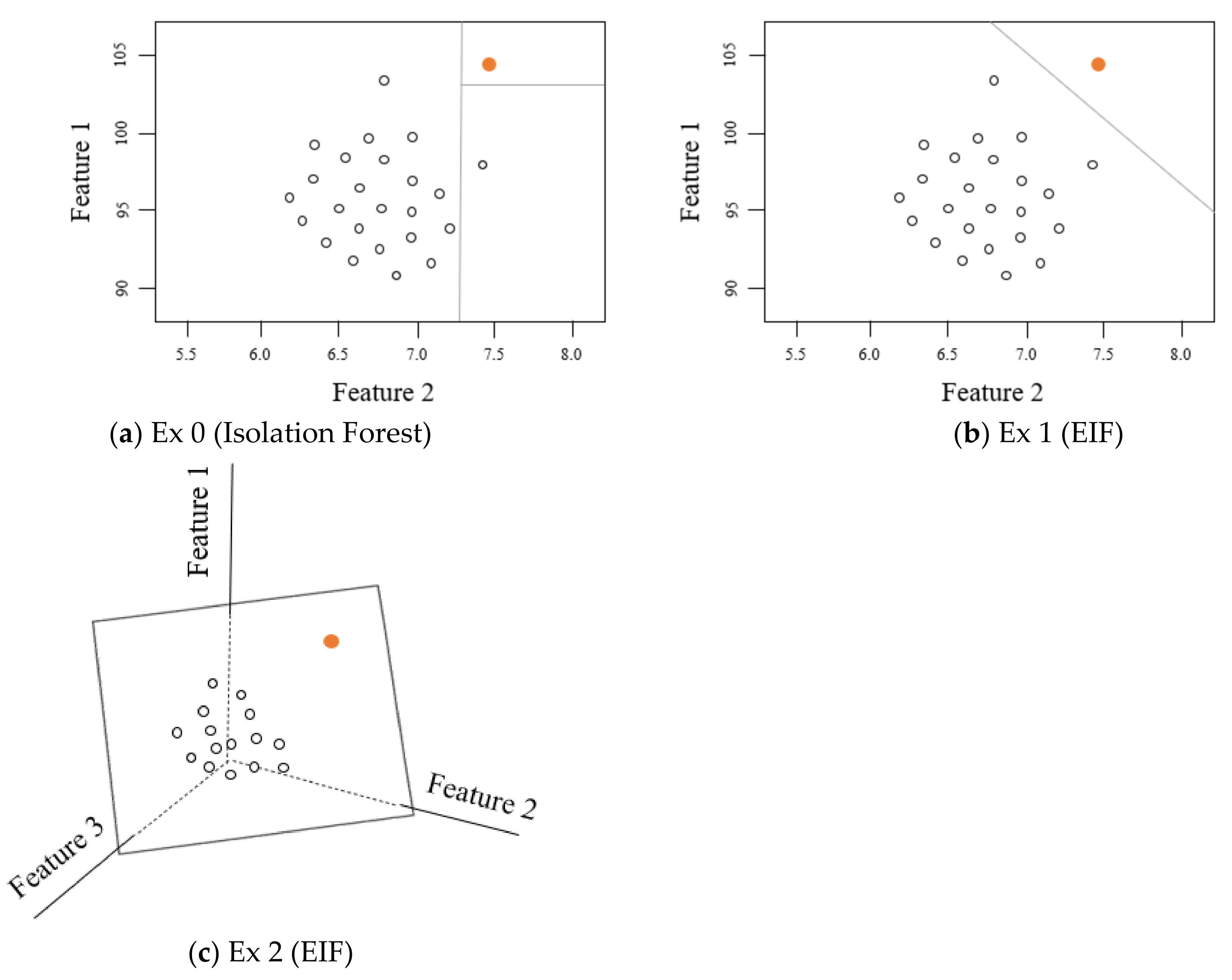
Isolation forest (IF) [19] is a well-known unsupervised learning method that has been used to detect anomalies or faults [18,20,21]; it is a novel method of identifying data abnormalities, unlike the k-nearest neighbor (k-NN) classifier and support vector machine (SVM), which use distance-based classifications. The recently proposed extended isolation forest (EIF) adds an additional degree of freedom to the parallel-axis split of the IF and helps rapid isolation of the dataset [22,23]. Therefore, we investigated FD problems with the EIF model for semiconductor etch process/equipment faults with the expectation of improved accuracy and speed compared with the conventional IF approach.

In this study, we attempted to find key features that can diagnose MFC failure using OES data and other sensor data attached to the chamber when the MFC does not recognize its own failure. Moreover, using the EIF model, we attempted to demonstrate that these features were effective in etch process/equipment FD. In addition, we attempted to demonstrate that the EIF used for FD is better to the IF in terms of accuracy and speed. Furthermore, by demonstrating the utility of electron temperature data for etch process/equipment FD, we attempted to provide additional information for FD and FC related to MFC.

2. Background

2.1. Principle and Characteristics of Isolation Forest

The IF is an unsupervised learning model that diagnoses anomalies via isolation methods, unlike the distance or density measurement methods. In addition, because of the use of subsampling techniques, model training can be performed using only data subsets. Therefore, training can be completed quickly with limited amounts of data. In addition, even if high-dimensional data with multiple features are used, the algorithm performs well for abnormality diagnosis.

To understand the IF anomaly diagnosis algorithm, we assumed that data were collected from two sensors for 25 s each at 1 s intervals. The data from one sensor was labeled as Feature 1, while data from the other was labeled as Feature 2. These data are shown as a scatter plot in Figure 1; each data point is referred to as an instance. Assume that we continue to draw lines to separate one instance from the other 24 instances. There are no rules for drawing the lines, and random values are chosen while lines are drawn for the maximum and minimum values of instances for randomly chosen features. The instances that are close to the center require large numbers of line segments to distinguish them from other instances. Thus, the instances approach normal data as the number of line segments increases, and the instance approaches abnormal data as the number of line segments decreases. To diagnose the abnormality of the given data, the IF anomaly diagnosis algorithm employs a similar principle.

2.2. Principle and Characteristics of EIF

Anomaly diagnosis with the EIF algorithm is similar to that with the IF in that as sooner an individual instances are separated from other instances, they are closer to the anomaly data. However, when separating one instance from another in the IF, only one randomly chosen feature is considered, whereas in the case of EIF, two or three features are considered simultaneously. In the EIF algorithm, the case in which two features are considered simultaneously is referred to as the 1st extension (Ex 1), and the case where three features are considered simultaneously is referred to as the 2nd extension (Ex 2). Thus, the original IF is the zero extension (Ex 0) case. The EIF algorithm has the advantage of being able to isolate data that are far from normal data faster than the IF, as shown in Figure 2b. As a result, data outliers along the diagonal of the normal data cluster can be diagnosed more accurately.

$$(\overrightarrow{x}-\overrightarrow{p})·\overrightarrow{n}\le 0$$

(1)

Equation (1) is used in the EIF algorithm to consider two or three features simultaneously. As a result, the instances are classified based on whether the vector product result is greater or less than zero. In this case, $\overrightarrow{n}$ is used for the slope of the straight line, and $\overrightarrow{p}$ is used to move the straight line. Further, $\overrightarrow{x}$ represents the value of the instance as a vector.

3. Experiments

To prove the proposed FD concept in this study, we demonstrate an example of a fault with gradual degradation of the MFC over the time of use. The MFC guides the exact amount of process gas flow rate to be fed into the chamber in units of standard cubic centimeters per minute, and appropriate calibration is required according to the range of gas flow amounts required. When a miscalibration occurs from usage over time, the amount of gas fed into the chamber induces a drift in the process results. When extended over time, unnoticed process shifts are induced. Because the observation of faults induced by the semiconductor equipment that follow a stochastic probability cannot be intentional, we devised a fault scenario where the MFC degraded over time with intentional adjustment of the gas flow amounts of SF₆. A series of etch process runs were performed for various cases of the miscalibrated MFC, and the equipment status variable identification data (SVID) and OES data were collected in real time.

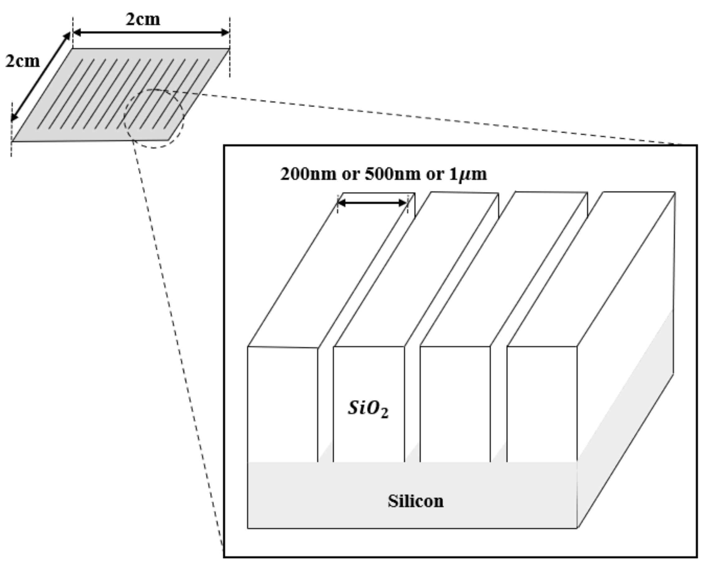
The equipment employed in this research was a 300 mm inductively coupled plasma (ICP) etching system, which consists of a 13.56 MHz RF source and bias power system. Silicon wafer coupons (2 × 2 cm²) with a silicon dioxide etch mask were prepared for the etching experiments. The sample coupons contain line and space patterns of 200 nm, 500 nm, and 1 μm to enable practicing the shallow trench isolation (STI) process, as shown in Figure 3.

The process condition for the silicon trench etch was adopted from the previously determined best known method (BKM) recipe [18]. The baseline process recipe contained 800/50 W of RF source/bias power, a mixture of O₂ (124 sccm) and Ar (10 sccm) with a base pressure of 20 mTorr, and the amount of SF₆ gas flow was varied from 158 to 194 sccm in steps of 2 sccm, as summarized in

Table 1. Description of the etch process recipe.

Etch Process Recipe
Power [W]	Source	800
	Bias	50
Gas [sccm]	O2	124
	Ar	10
	SF6	158, 160, 162, …, 176, …, 190, 192, 194
Chuck Temperature [°C]		25
Chamber pressure [mTorr]		20
Remarks		Each etch process is run for 180 s

. During the process, the acquired equipment SVID and OES data were stored in database servers every second. From the process baseline with 176 sccm of SF₆ (normal process), we set nine fault cases from 174 sccm to 158 sccm in decrements of 2 sccm and nine fault cases from 178 sccm to 194 sccm in increments of 2 sccm. Note that the maximum range of the MFC for SF₆ was 500 sccm with 1 sccm of control by the equipment operation SW.

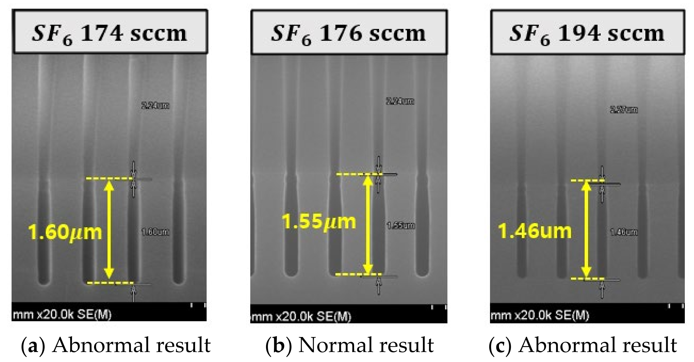
Each fault case was repeated three times to ensure data repeatability in the experiments. The total number of experimental runs was 66 etch runs with 12 normal processes and 54 abnormal processes. Sample scanning electron microscope (SEM) images of the silicon etch results from this experiment are presented in Figure 4. It can be seen that even a small change in the amount of SF₆ gas injected during the process affects the etch depth.

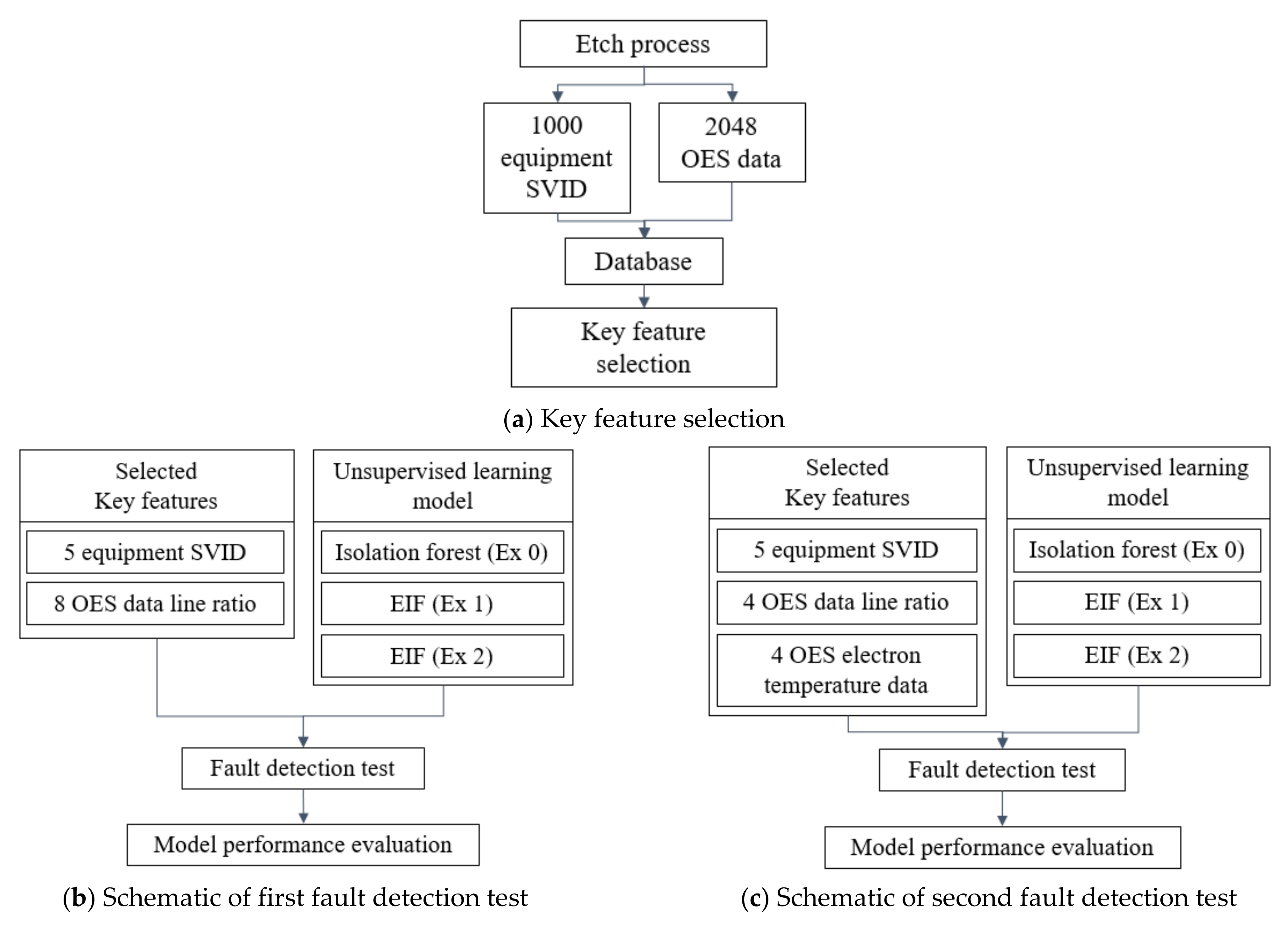
Using the aforementioned equipment SVID and OES data, we first selected the key features that were sensitive to changes in the flow rate of the SF₆ gas. Second, using the selected key features and acquired dataset, we compared the accuracies and speeds of the IF and EIF models. Finally, we investigated whether the electron-temperature-related features calculated from the OES datasets could aid detection of process/equipment faults in terms of plasma parameter metrics, as shown in Figure 5.

The violin plot was used for key feature selection, and the accuracy of each model was compared using the precision, recall, and F1 scores. In addition, to evaluate the performances of some models, the equipment SVID and OES data acquired for the BKM process were labeled as normal, and those acquired for recipes other than the BKM process were labeled as abnormal.

4. Results and Discussion

According to the designed fault scenarios in the MFC miscalibrations, we performed 66 silicon etch runs, and two types of datasets were collected in real time. The first is equipment SVID comprising more than a thousand parameters, including the operational set values and current values of various components related to RF power, pressure, gas flow, and electrostatic chuck. The second is OES data, which give a plasma emission spectrum of 2048 points (the resolution of OES is approximately 0.32 nm), with important peaks related to the atomic and molecular energy transitions between the excitation and ionization of constituent species in the plasma. 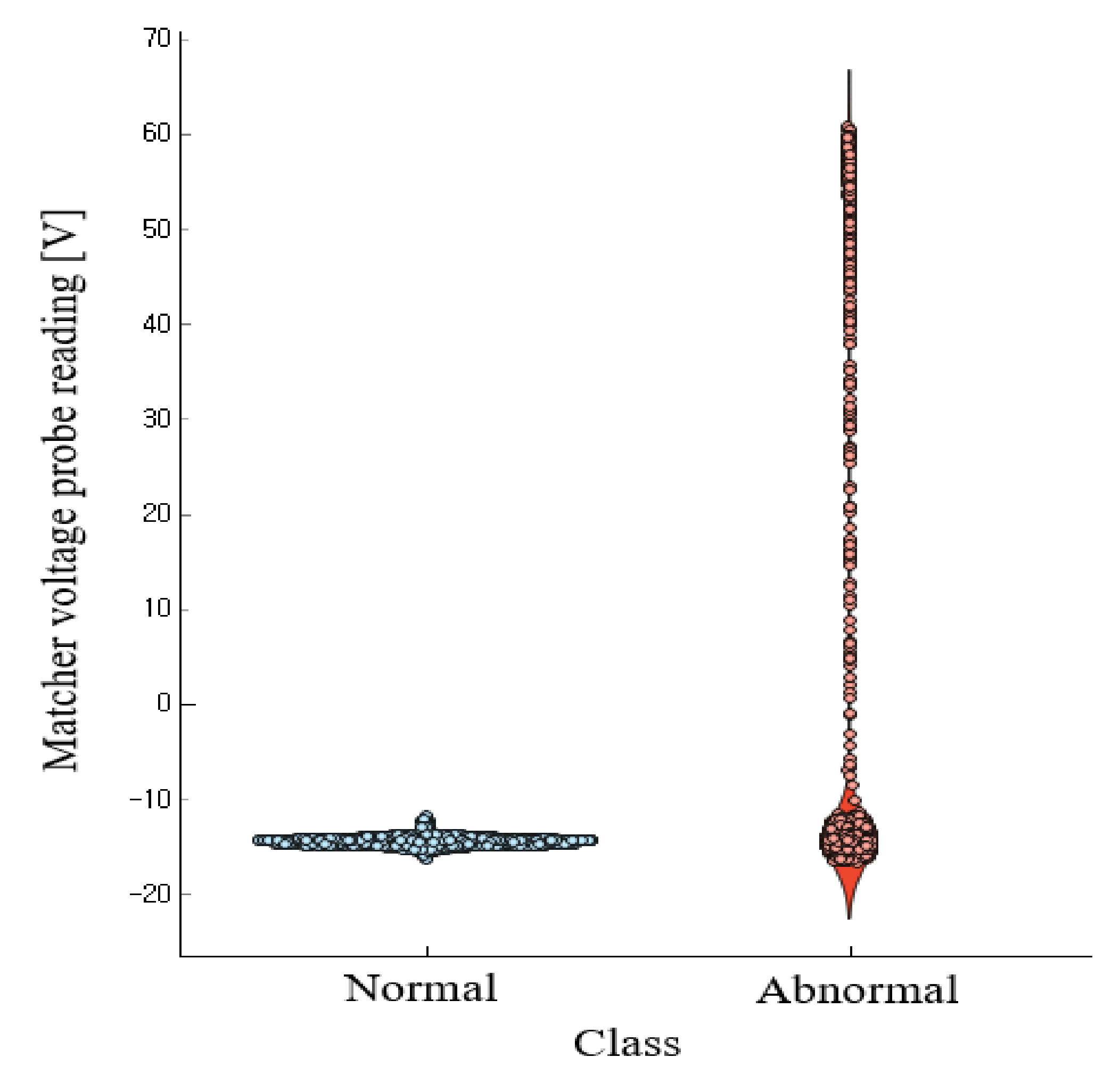Initially, we used our domain knowledge of the plasma etch equipment and selected a few tens of equipment parameters related to the MFC miscalibration scenarios; the distributions of the selected parameters were then investigated to compare the sensitivity to changes in the gas flow rate of SF₆ between the normal and abnormal processes. When less amount of gas flow was fed into the vacuum chamber, the chamber pressure decreased owing to the lack of particles under the assumption that the pumping speed and throttle valve were fixed while the deficit of the process gas could be easily detected. However, high-end semiconductor manufacturing equipment are often equipped with fully automated features, including an automatic pressure controller, and the gate valve position control can be used to maintain the desired chamber pressure. In the same manner, reduced/increased amounts of the gas flow rate contribute to the amount of ionization that affect plasma resistivity or conductivity and in turn the plasma impedance. In RF plasma equipment, the RF matching unit called a matcher helps maintain the predetermined RF impedance to maximize RF power delivery from the RF generator to the plasma via adjustment of the capacitance of the vacuum variable capacitor in the matcher. When the amount of gas flow changes, the plasma impedance changes, and the capacitor position of the matcher is changed to compensate for the distorted RF impedance. An illustration of the significant variable selection using a violin plot is shown in Figure 6.

In the silicon etch process, the plasma generated with a mixture of SF₆/O₂/Ar gases forms fluorine and oxygen ions and radicals that react with the silicon surface to form volatile products of silicon fluoride, and the augmented oxygen helps the silicon etch process by preventing formation of inhabitant of etch byproducts. The advantage of OES is that it is a noninvasive plasma monitoring method; however, the optical emission intensity depends on the detected photon count with a charged coupled device (CCD), and these values are measured in terms of arbitrary units. To alleviate this concern, actinometry application has been suggested as a useful method for the analysis of plasma optical emission data [24]. Thus, we selected the five most significant variable equipment parameters and eight most significant line ratios of the OES data relative to the fluorine and oxygen species, as presented in

Table 2. Selected key feature data.

Key Feature List
Category	Feature Name
Tool data	RF matcher voltage probe [V] Chuck ESC total voltage [V] Fore line manometer voltage [mV] Throttle valve position [A.U.] Pendulum valve position [A.U.]
OES data line ratio	F685 nm/Ar750.4 nm F703 nm/Ar750.4 nm O777 nm/Ar750.4 nm O844 nm/Ar750.4 nm	F685 nm/Ar811.5 nm F703 nm/Ar811.5 nm O777 nm/Ar811.5 nm O844 nm/Ar811.5 nm

.

Once we selected the most significant parameters of the two data sets, the EIF model was established and evaluated using the precision, recall, and F1 score metrics. The precision metric is defined as the ratio of actual abnormalities to those considered abnormal by the model; recall refers to the proportion of data that a model judges as abnormal among the data with actual abnormalities. The F1 score indicates the harmonic average of the precision and recall values, which are calculated using the equations below:

$$\mathrm{recision}=\frac{\mathrm{True}\mathrm{Positive}}{\mathrm{True}\mathrm{Positive}+\mathrm{False}\mathrm{Positive}}$$

$$\mathrm{Recall}=\frac{\mathrm{True}\mathrm{Positive}}{\mathrm{True}\mathrm{Positive}+\mathrm{False}\mathrm{Negative}}$$

$$\mathrm{F}1 \mathrm{score}=2\times \frac{\mathrm{Precision}\times \mathrm{Recall}}{\mathrm{Precision}+\mathrm{Recall}}$$

If the number of normal and abnormal data are similar, the model is validated using the accuracy value. However, the data used in this experiment are unbalanced in terms of the number of normal and abnormal data points (18.18% normal and 81.81% abnormal data); thus, the F1 score is more explainable. For performance comparisons, the best hyperparameters for the EIF and IF models were selected using the grid-search method. In this case, four parameters (number of trees, sample size, depth limit, and threshold) were applied to each model, and a grid search was performed by substituting the values in

Table 3. Parameter range of each variable used in the grid search of the EIF and IF models.

Model Parameter	Ranges
Number of trees	50 to 500 with an incremental step of 50
Sample size	50 to 500 with an incremental step of 50
Tree’s depth limit	2 to 20 with an incremental step of 2
Threshold	0.21 to 0.99 with an incremental step of 0.01

.

Each model was subjected to FD tests with the chosen hyperparameter values, and the results shown in

Table 4. Fault detection result of each model.

Model	Precision	Recall	F1 Score	Diagnostic Time(s)
Extended Isolation Forest (Ex 2)	0.955	0.982	0.968	0.07
Extended Isolation Forest (Ex 1)	0.963	0.966	0.964	0.11
Isolation Forest (Ex 0)	0.955	0.957	0.956	0.12
Remarks	EIF (Ex 2)—No. of trees: 300, Sample size: 400, Depth limit: 15, Threshold: 0.49
	EIF (Ex 1)—No. of trees: 350, Sample size: 500, Depth limit: 18, Threshold: 0.49
	IF (Ex 0)—No. of trees: 400, Sample size: 450, Depth limit: 18, Threshold: 0.45

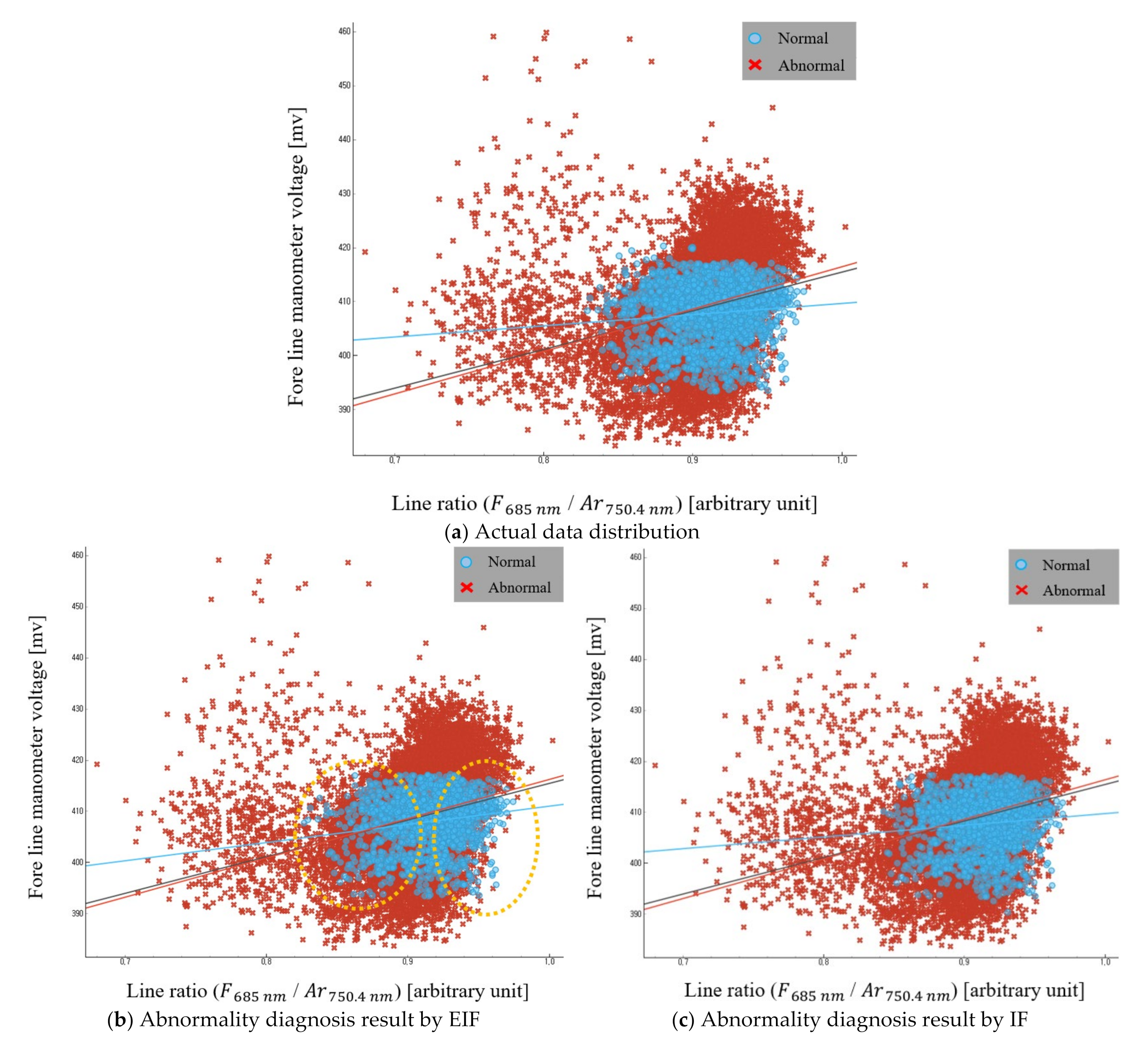
are the average values obtained after repeating the FD test for each model 10 times. In Table 4, the diagnostic time refers to the time required to diagnose a fault using each model for data obtained from a single 180 s etch process. From a comparison of the F1 scores, it is clear that the EIF model, which considers two or three variables simultaneously in FD, outperforms the IF model. Hariri et al. confirmed that unlike the IF model, the EIF model could distinguish the degree of data abnormality sufficiently along the diagonal of the normal data [22]. From the actual experimental results, it can be seen that the EIF judges the abnormality of the data on the diagonal of the center of the normal data better than the IF, as shown in Figure 7. The diagnosis speed of the EIF model is also high because better performance could be achieved with fewer trees than the IF model.

From the above FD test, when the difference between the set value and flow rate of the SF₆ gas flowing into the chamber was less than 2 sccm, the FD models did not recognize this difference well through the other sensor data. However, when the difference between the SF₆ gas set value and flow rate was more than 4 sccm, it was confirmed that the models could recognize the difference well through the other sensor data. These results demonstrate the usefulness of the OES data for representing plasma status in terms of gas flow rate variation, and the EIF shows improved accuracy and computational speed compared to the conventional IF method. The improvement with EIF is only slight, but both EIF and IF are useful for FD in semiconductor process/equipment data.

Recent advancements in the analysis of OES data have shown that appropriate selection of the OES peaks and their ratios with respect to the argon peaks are useful for deriving plasma information, such as the electron density and electron temperature [25]. Electron density is a function of the atomic/molecular ionization by the amount of collision of the gas species, and the electron temperature is a measure of the total energy of the electrons in the plasma. The electron temperature is also a function of the electron density under a given condition, but other factors such as the amount of applied RF power and pressure related to the amount of collisions are also considered. In our experiments, we only considered the gas flow amounts in the chamber; however, it is worth investigating whether the electron temperature calculated from the acquired OES data is useful for FD of gas flow variations.

We used the OES data to generate features related to various electron temperatures and chose four data values from among these features that were sensitive to changes in the SF₆ flow rates. The electron temperature of the SF₆/O₂/Ar plasma was calculated using the Corona model of electron temperature calculation and the information in

Table 5. Light wavelengths (nm) generated during Ar ($3p^{5}4p\to 3p^{5}4s$) transformation.

Exited Levels	Resonance Levels		Metastable Levels
	$1{\mathit{s}}_{2 }\left(\mathit{J}=1\right)$	$1{\mathit{s}}_{4 }\left(\mathit{J}=1\right)$	$1{\mathit{s}}_{3 }\left(\mathit{J}=0\right)$	$1{\mathit{s}}_{5 }\left(\mathit{J}=2\right)$
$2p_{1 }\left(J=0\right)$	750.39	667.73	-	-
$2p_2 \left(J=1\right)$	826.45	727.29	772.42	696.54
$2p_3 \left(J=2\right)$	840.82	738.40	-	706.72
$2p_4 \left(J=1\right)$	852.14	747.12	794.82	714.70
$2p_5 \left(J=0\right)$	858.01	751.47	-	-
$2p_6 \left(J=2\right)$	922.45	800.62	-	763.51
$2p_7 \left(J=1\right)$	935.42	810.37	866.79	772.38
$2p_8 \left(J=2\right)$	978.45	842.46	-	801.48
$2p_9 \left(J=3\right)$	-	-	-	811.53
$2p_{10} \left(J=1\right)$	1148.8	965.78	1047.0	912.30

regarding the wavelength of light generated during Ar ($3p^{5}4p\to 3p^{5}4s$) transformation.

$$\frac{I_{{\mathrm{Ar}}_1}}{I_{{\mathrm{Ar}}_2}}=\frac{n_e·n_{\mathrm{Ar}}·Q_{\mathrm{EXC}}^{\mathrm{Ar}(3p_1)}}{n_e·n_{\mathrm{Ar}}·Q_{\mathrm{EXC}}^{\mathrm{Ar}(2p_1)}}=C·\frac{Q_{\mathrm{EXC}}^{\mathrm{Ar}(3p_1)}}{Q_{\mathrm{EXC}}^{\mathrm{Ar}(2p_1)}} \fallingdotseq \mathrm{EXP}\left(-\frac{∆E}{T_e}\right)$$

$$T_{e }\fallingdotseq \frac{-∆E}{\ln \left(I_{{\mathrm{Ar}}_1}/I_{{\mathrm{Ar}}_2}\right)}$$

$$T_{e }\fallingdotseq \frac{-\left(\mathrm{Excited}\mathrm{level}\mathrm{energy}\mathrm{of} {\mathrm{Ar}}_1-\mathrm{Excited}\mathrm{level}\mathrm{energy}\mathrm{of} {\mathrm{Ar}}_2\right)}{\ln \left(I_{{\mathrm{Ar}}_1}/I_{{\mathrm{Ar}}_2}\right)}$$

where I is the emission intensity of the corresponding wavelength, T_e is the electron temperature, ΔE is the difference in threshold energy levels between the two selected wavelengths. Moreover, ΔE is similar with the difference of the excited energy levels of the two wavelengths. To calculate the electron temperature, we developed a program [26] that generates all possible electron temperature values using the data of Ar wavelengths from Table 5. Thereafter, using the extreme gradient boosting (XGB) regression, the target value was set as SF₆ MFC sensor actual reading and regression was performed with the electron temperature data. Then, using the permutation importance, four electron temperature values that had the greatest influence in the regression process were selected as the key features. To observe if the selected electron temperature values are useful for process/equipment FD, the four chosen features were mixed with some of the key features noted in Table 2, as shown in

Table 6. Selected key feature data.

Key Feature List
Category	Feature Name
Tool data	RF matcher voltage probe [V]
	Chuck ESC total voltage [V]
	Fore line manometer voltage [mV]
	Throttle valve position [A.U.]
	Pendulum valve position [A.U.]
OES data line ratio	F685 nm/Ar750.4 nm
	F703 nm/Ar750.4 nm
	O777 nm/Ar750.4 nm
	O844 nm/Ar750.4 nm
OES electron temperature (Te) data	Te calculated by Ar738.585 nm and Ar772.856 nm [eV]
	Te calculated by Ar738.906 nm and Ar772.856 nm [eV]
	Te calculated by Ar772.539 nm and Ar714.644 nm [eV]
	Te calculated by Ar772.856 nm and Ar714.644 nm [eV]

, and FD tests were performed. For accurate comparisons, we used the same hyperparameter values as those noted in Table 4.

The results in

Table 7. Fault detection results of each model.

Model	Precision	Recall	F1 Score	Diagnosis Time (s)
Extended Isolation Forest (Ex 2)	0.958	0.980	0.969	0.07
Extended Isolation Forest (Ex 1)	0.964	0.968	0.966	0.10
Isolation Forest (Ex 0)	0.956	0.973	0.964	0.12
Remarks	EIF (Ex 2)—No. of trees: 300, Sample size: 400, Depth limit: 15, Threshold: 0.49
	EIF (Ex 1)—No. of trees: 350, Sample size: 500, Depth limit: 18, Threshold: 0.49
	IF (Ex 0)—No. of trees: 400, Sample size: 450, Depth limit: 18, Threshold: 0.45

are the average values of the results obtained after repeating the FD tests for each model 10 times. Compared with the results in Table 4, there are slight improvements in the performances of Ex 1 and Ex 2 based on the F1 scores, and an improvement of approximately 0.84% is observed for the F1 score of the IF model. The reason for the improvements in the above results is that the distinction between normal and abnormal electron temperatures is clearer than the line ratio, as shown in Figure 8. This electron temperature was proportional to the increase of the SF₆ flow rate. This is thought to be because, when the atmospheric pressure in the chamber was constant at 20 mTorr, increasing the flow rate of SF₆ produced more reactive fluorine, and as fluorine reacted with other gases, more electrons and gas ions affected by the RF power were produced. As a result, if the line ratio and electron temperature data are used together, the FD performance of the model is expected to improve. Furthermore, we believe that using the features in Table 6 will aid FC of SF₆ related MFC fault.

5. Conclusions

In this study, we performed process/equipment FD using OES data and EIF approach to identify three main results as follows. First, it was confirmed that when the equipment did not recognize MFC failure, the OES and other sensors attached to the chamber could be used to detect MFC failure. Second, we compared the IF and EIF methods, both of which are unsupervised learning models, and confirmed that the EIF approach diagnosed anomalies 1.7 times faster than the IF and had 1.26% higher accuracy. Third, when electron temperature data were additionally used for etch process/equipment FD, the accuracy of the model was slightly improved by a maximum of 0.84%.

In the above process, we focused on identifying key features that can improve the accuracy of FD and classify SF₆-related MFC failures. We expect that this study will aid FD and FC of SF₆ related MFC in the industrial field. However, the causes of process/equipment failure are numerous, and accurate FC must be performed for root cause analysis. Thus, in the future, we intend to continue finding key features that are sensitive to changes in the parameter values by acquiring data with intentional changes single parameter values in the etch process. In addition, by combining the EIF with depth-based isolation forest feature importance (DIFFI) algorithm [27], which lists features with high probabilities of anomalies in sequential order, we intend to use the EIF for not only FD but also FDC in various fault scenarios.