A Parallel Deep Reinforcement Learning Framework for Controlling Industrial Assembly Lines

Abstract

Decision-making in a complex, dynamic, interconnected, and data-intensive industrial environment can be improved with the assistance of machine-learning techniques. In this work, a complex instance of industrial assembly line control is formalized and a parallel deep reinforcement learning approach is presented. We consider an assembly line control problem in which a set of tasks (e.g., vehicle assembly tasks) needs to be planned and controlled during their execution, with the aim of optimizing given key performance criteria. Specifically, the aim will be that of planning the task in order to minimize the total time taken to execute all the tasks (also called cycle time). Tasks run on workstations in the assembly line. To run, tasks need specific resources. Therefore, the tackled problem is that of optimally mapping tasks and resources to workstations, and deciding the optimal execution times of the tasks. In doing so, several constraints need to be respected (e.g., precedence constraints among the tasks, constraints on needed resources to run tasks, deadlines, etc.). The proposed approach uses deep reinforcement learning to learn a tasks/resources mapping policy that is effective in minimizing the resulting cycle time. The proposed method allows us to explicitly take into account all the constraints, and, once training is complete, can be used in real time to dynamically control the execution of tasks. Another motivation for the proposed work is in the ability of the used method to also work in complex scenarios, and in the presence of uncertainties. As a matter of fact, the use of deep neural networks allows for learning the model of the assembly line problem, in contrast with, e.g., optimization-based techniques, which require explicitly writing all the equations of the model of the problem. In order to speed up the training phase, we adopt a learning scheme in which more agents are trained in parallel. Simulations show that the proposed method can provide effective real-time decision support to industrial operators for scheduling and rescheduling activities, achieving the goal of minimizing the total tasks’ execution time.

1. Introduction

Machine Learning (ML) has emerged as one of the key enablers for improving efficiency and flexibility in industrial processes and represents a pillar of the Industry 4.0 paradigm [1]. In particular, Deep Reinforcement Learning (DRL) has attracted the interest of scheduling and operational research communities as it allows us to efficiently tackle large-scale combinatorial optimization problems requiring fast decisions [2,3]. Indeed, industrial processes are complex, dynamic, cyberphysical systems subject to disturbances related to uncertainties and delays affecting all the stages of products’ supply chains. Classic optimal control-based approaches do not provide enough flexibility in the presence of disturbances or deviations from nominal conditions. On the other hand, after a proper training phase, DRL techniques allow us to solve complex decision-making problems in real time. However, the duration of the said training phase is often very long, and its reduction represents an important research line in the field of DRL [4,5].

The problem considered in this work consists of controlling industrial assembly lines. The objective of an assembly line is to perform a given set of tasks (or jobs). Tasks are processed by workstations which are the machines or areas in which components/products are created or assembled. The problem of assigning tasks (and resources) to workstations in an efficient way is known in the literature as the Assembly Line Balancing Problem (ALBP). ALBPs can be characterized in terms of the factory layout (i.e., the directed graph modelling the interconnections between workstations), the peculiarities of the products to be assembled/created or the types of considered constraints. Over the years, the control of assembly lines has gathered the attention of many researchers, which has translated into a huge number of scientific articles focusing on a variety of ALBPs instances. This, in turn, has led to numerous ALBPs’ classification schemes.

A first classification divides the literature into simple and generalized ALBP instances (SALBP and GALBP, respectively). SALBPs are characterized by strong assumptions about the nature of the assembly line and the product to be created. Four basic SALBP instances have been identified [6]. SALBP-F instances consist of deciding if a feasible balance exists given the number of workstations and the cycle time (i.e., the time required by each workstation to process tasks). SALBP-1 and SALBP-2 instances minimize the number of workstations given a fixed cycle time and vice versa, respectively. SALBP-E, finally, simultaneously minimizes the number of workstations and the cycle time. Over the years, GALBPs have gained a significant relevance in the industrial world as they allow us to capture more realistic operational scenarios. In [7], the authors propose a classification of GALBPs based on tuples $(\alpha ,\beta ,\gamma )$ where $\alpha$ captures the characteristics of tasks’ precedence constraints, $\beta$ specifies workstations and assembly line characteristics, and $\gamma$ captures the different optimization objectives.

More recent works (e.g., [8,9]), propose a hierarchical classification scheme based on three characteristics: the number of models of the product to be created, the nature (deterministic or stochastic) of tasks’ execution times, and the characteristics of the factory layout (e.g., straight lines, parallel lines and U-shaped lines). With respect to the first element, single-model APBPs refer to a scenario in which a single product is processed by workstations. Multimodel ALBPs, instead, refer to a scenario in which multiple products are created in batches; in other words, a generic workstation can create a single product, and, after a proper set-up phase, can create a different product. If workstations do not require such a set-up phase for creating different products, the ALBP instance is referred to as mixed-model ALBP.

In this work, a complex GALBP instance will be considered. More specifically, no assumptions are made on the factory layout nor on the tasks’ precedence constraints. Furthermore, a mixed-model assembly line is considered. The objective of the proposed solution consists of minimization of the total cycle time. To solve this problem, a DRL framework has been developed. The proposed DRL framework adopts a parallel training phase to solve the aforementioned DRL issues. Similarly to what conducted in [10], the proposed parallel training is based on a shared representation of the environment. As further detailed in the next sections, each DRL agent proposes a set of candidate actions and then a centralized control logic combines said actions into a single command which is implemented, producing a state variation in the environment. Simulations have proven that the adoption of said control logic allows for the generation of high-quality control actions since the beginning of the training phase.

The reported research has been carried out in the context of the H2020 SESAME project [11], coordinated by ArianeGroup. The project aims at increasing European space access capabilities by exploiting data science. In this context, the optimization of the integration activities to be performed at the French Guyana Kourou spaceport has been identified as crucial for addressing the aforementioned issues.

The remainder of the paper is organized as follows. Section 2 presents a review of the literature with respect to the considered assembly line problem and parallel/distributed DRL approaches. Section 3 formalizes the problem from a mathematical viewpoint. Section 4 describes the proposed parallel DRL framework for achieving a faster training phase. Section 5 presents the numerical simulations, and finally, Section 6 wraps up the presented work and outlines limitations and future improvements.

2. Related Works and Paper Contributions

As already mentioned, assembly line balancing problems (ALBPs) are combinatorial optimization problems consisting of deciding how to distribute a given set of activities/tasks across a given set of workstations. Said workstations, whose interconnection defines the so-called factory layout, are the places or machines which, by exploiting the available resources, allow us to process the tasks to be completed for achieving a given industrial manufacturing goal.

In [12], the authors present a systematic review of the literature, analysing scientific articles published from 1990 to 2017. Among other aspects, the authors highlight how the research lines in this field have evolved. In particular, the study reports that while in the 1990–2000 period, research activities focused on a single instance of ALBPs (i.e., the single-ALBP in which a single product is assembled) and on heuristic solution methods, and after 2000, more attention has been devoted to other ALBPs instances and on meta-heuristics. In addition, starting from the 2010s, ALBP instances which also consider the issue of assigning resources (e.g., equipment, workers, raw materials) gathered a significant relevance. Indeed, the ALBP problem considered in the present work belongs to the latter research line, since, at each discrete time instant, it simultaneously considers the problem of assigning tasks and resources to workstations.

A deep review of exact methods and (meta)heuristics developed for the industrial sector is beyond the scope of this work. For an insight on the different ALBP instances and relative solution methods, the reader can refer to the following review articles: [8,9,13]. In [14], the authors discuss the application of exact methods, heuristics and machine-learning techniques for solving combinatorial problems. In particular, the authors point out that said techniques can be successfully applied for solving small- and medium-sized problems, while for large-scale problems, DRL techniques should be adopted. Hence, the remainder of this section is devoted to reviewing the literature with respect to the adoption of RL (Section 2.1) and DRL (Section 2.2) techniques for addressing ALBPs. Furthermore, parallel and distributed DRL approaches will also be discussed (Section 2.2.1), since they provide the baseline of the framework adopted by the solution proposed in this work.

2.1. RL Approaches

In [15], the authors address the (re)scheduling problem for NASA ground operations by means of ML algorithms in presence of time constraints. The adoption of ML proved to be useful for reducing the time required to prepare a launch campaign at the Kennedy spaceport. In particular, the authors train an artificial agent (in charge of solving an ALBP) by means of a heuristic iterative repair method. In [16], the authors address a similar problem considering both time and resource constraints. The aim of this work consists of finding the shortest conflict-free schedule for all the activities. To achieve this, the authors have adopted a temporal difference Reinforcement Learning (RL) algorithm for training a neural network in charge of learning how to introduce repair actions into the tasks’ schedule. A RL-based approach for solving a scheduling problem has also been addressed in [17]. The authors, by exploiting the Open AI Gym toolkit [18], have developed an RL framework for training an artificial agent, evaluating its performances with respect to classic operations research problems. In particular, the rewards obtained by the RL agent are computed based on heuristics, which allows for reducing the computational cost of the proposed solution. The problem of reducing computational costs of RL-based scheduling algorithms has been also addressed in [19], in which the authors addressed a real-time scheduling problem in the context of earth observation services. The proposed solution combines the strengths of RL and classic operations research techniques. In particular, by means of an Markov Decision Process (MDP) formulation of the problem, an RL algorithm is used to reduce the computational costs associated with the dimensions of the solution space, while a dynamic programming problem is set up for solving the sequencing and timing problems. Results show that the combination of the two mentioned techniques allows for reducing training times and achieving better generalization capabilities. In [20], the authors address the scheduling problem considering the presence of resources to be shared by different clients in a data centre. The authors developed a time-varying RL formulation of the problem and tested the proposed solution on real-time production data metrics from Google and Alibaba: the simulations proved a significant improvement with respect to resource usage.

2.2. DRL Approaches

In [21], the authors developed a smart scheduling agent using a DRL algorithm. An interesting characterisc of the proposed approach is its ability to deal with uncertainties such as random task arrivals and equipment damages. Similarly, in [22], the authors tackle industrial scheduling problems in presence of uncertainties and propose a DRL proximal policy optimization algorithm. Many researchers have investigated the adoption of a deep deterministic policy gradient approach for dealing with problems characterized by continuous environments. As an example, in [23], the authors developed a deep deterministic policy gradient algorithm which, in contrast to deep Q network (DQN) algorithms, can be applied for continuous state and action spaces. The authors proved that the proposed algorithm performs similarly to state-of-the-art DQN algorithms. A similar approach has been adopted in [24], where the authors applied a deep deterministic policy gradient algorithm for solving a scheduling problem. In [25], the authors developed a graph neural network-based method to solve generic combinatorial optimization problem. More in detail, the proposed solution adopts an offline DQN-based training phase for learning optimal policies in simulated environments; at run time, the trained Q-network is embedded in a modified version of the Monte Carlo tree search method, guaranteeing more robust solutions. Indeed, the developed approach benefits from the generalization abilities learned during the offline training phase and the solutions’ robustness obtained by means of the online tree search.

The literature review performed so far justifies the following statements:

• ALBPs are in general NP-hard problems which naturally arise in industrial processes; many instances have been formalized and most of the solutions are instance-driven, i.e., tailored to the specific use case addressed;
• Several advanced algorithms have been developed for supporting exact methods; computational costs’ reduction has also been addressed by means of heuristics and genetic algorithms; however, with the explosion of exploitable data and the consideration of more complex industrial problems, said improvements are not enough to deal with more complex ALBP instances;
• Several ML-based approaches have been proposed and applied to industrial problems; although RL-based approaches allow us to learn optimal policies also in a model-free setting, they can be applied to small- and medium-sized problems or to simple ALBP instances;
• Large-sized problems and complex ALBP instances can be successfully addressed by DRL techniques; however, in this context, the duration of the training phase and the quality of the solutions represent crucial aspects which still need to be investigated.

Due to these considerations, many researchers have focused on developing distributed, parallel and multiagent DRL approaches for overcoming the limitations highlighted in ($\delta$). The next subsection will review this latter class of approaches.

2.2.1. Parallel and Distributed DRL Approaches

In [26], the authors describe a framework in which a number of actor–learners are used in parallel on a single machine. Since the actor–learners run in parallel on a single multicore CPU, there is no need to exchange information between several machines. The authors point out that the adoption of multiple actor–learners in parallel allows us to (i) stabilize and to (ii) reduce the required time of the training phase. In particular, the adoption of different exploration strategies allows us to avoid the usage of replay memories adopted, for example, by the DQN training algorithm. The proposed DRL framework optimizes the decisions of the DRL controllers by means of an asynchronous gradient descent method. More in detail, each actor–learner interacts with its own instance of the environment, and after computing its gradient, updates shared parameters in an asynchronous way. A similar solution has been presented in [27]: the authors describe a parallel DRL algorithm able to run on a single machine. Contrary to what was conducted in the above-mentioned DRL framework, in this work, the parallel DRL algorithms runs on a GPU and not on a multicore CPU. In particular, the authors developed a parallel advantage actor–critic algorithm which proved to achieve state-of-art performances on benchmark problems with a few hours of training. In [28], the authors present a fully distributed actor–critic architecture for multitask DRL. An interesting characteristic of the proposed solution is that during the learning phase, the agents share details about their policy and parameters with their neighbours. In this respect, scalability is guaranteed, as the amount of data to be exchanged depends only on the number of neighbours and not on the total number of agents. In [29], the authors developed a multiagent DRL algorithm for minimizing energy costs associated with heating, ventilation and air-conditioning services in multizone residential buildings. The proposed solution is based on the idea that each thermal zone is associated with an agent, which, by interacting with the environment and the other agents, is able to learn the optimal policy. In this respect, scalability is guaranteed in terms of the number of thermal zones to be controlled. The authors adopted a multiactor attention critic approach allowing the agents to learn approximations of both policy and value functions. In particular, the interaction between the agents is governed by an attention mechanism, allowing them to consider in a selective way the information coming from the other agents. Said information is used to update, for each agent, the action-value function. The same problem has been addressed in [30], where the authors proposed a distributed multiagent DRL approach. Contrary to what conducted in the previous reviewed article, in this work the authors propose to train different agents for learning the cooling and heating set points. Simulations proved the benefits of this approach with respect to centralized and multizone approaches. Indeed, since the control actions can be divided in two groups (relative to heating and cooling actions), it makes sense to learn multiple policies for each zone. In the specific application scenario, this translates into learning a policy for warmer months and a different one for colder months.

2.3. Paper Contributions

The main contributions of this work can be summarized as follows:

• A complex ALBP instance envisaging (i) the presence of hard constraints concerning tasks, resources and workstations and (ii) the need for solving both tasks and resource assignment problems has been considered;
• A parallel DRL approach for solving the mentioned ALBP has been derived for reducing the time required by the training phase;
• Given the application sector (integration activities in the aerospace sector), hard constraints’ management has been embedded in the decision problem.

3. Problem Formalization

3.1. Assembly Line Balancing Problem

The ALBP instance considered in this work consists of assigning a given set of tasks $\tau$∈$\mathcal{T}$ and resources r∈$\mathcal{R}$ to a given set of workstations w∈$\mathcal{W}$. The objective of the proposed control algorithm is to minimize the total make span (i.e., the time required to finish all the tasks) while respecting all the constraints.

Each task ${\tau }_j$∈$\mathcal{T}$ is characterized in terms of (i) the first discrete time instance in which it can be processed $S_{{\tau }_j}$, (ii) the latest possible discrete time instant in which it must be completed $F_{{\tau }_j}$ and (iii) the number of discrete time steps required to process it $d_{{\tau }_j}$. The set of resources required to execute a given task ${\tau }_j$ is denoted with $R_{{\tau }_j}$. Resources can either be consumables (e.g., energy, water, chemicals, raw materials) or instruments (e.g., tools, operators, workers with specific). Each workstation $w_i$∈$\mathcal{W}$ is characterized in terms of its processing capabilities, i.e., in terms of the maximum number of tasks that can process in parallel $\overline{W_i}$.

The considered constraints can be grouped into three classes. Task constraints, ${\mathcal{T}}_{\mathcal{C}}$, specifying (i) the latest allowed start time $S_{{\tau }_j}$ and finish time $F_{{\tau }_j}$ for each task ${\tau }_j$ and (ii) dependence relations between tasks. The latter group of task constraints, also referred to as precedence constraints, allows us to capture the fact that a given task ${\tau }_{j_1}$ (i) must be finished before a given task ${\tau }_{j_2}$ can be processed or that (ii) it must start before a given task ${\tau }_{j_2}$ begins or that (iii) it must be finished before a given task ${\tau }_{j_2}$ can be finished, or, finally, that (iv) it must start before a given task ${\tau }_{j_2}$ can be finished. These type of constraints are referred to as Finish to Start (FS), Start to Finish (SF), Finish to Finish (FF) and Start to Finish (SF) constraints, respectively. Workstation constraints, ${\mathcal{W}}_{\mathcal{C}}$, specifying, for each workstation $w_i$∈$\mathcal{W}$, (i) which tasks and (ii) the maximum number of tasks that can be processed in parallel. Finally, resource constraints ${\mathcal{R}}_{\mathcal{C}}$, specify the type and quantity of resources needed to execute a given task ${\tau }_j$.

3.2. Proposed Markov Decision Process Framework

MDPs represent a useful mathematical framework for formalizing RL problems. Indeed, MDPs model decision processes in which part of the underlying dynamics is stochastic while part depends on the control actions taken by an agent. More precisely, MDPs are defined by means of the tuple $\langle \mathcal{S},\mathcal{A},P_a,R_a,\gamma \rangle$ where $\mathcal{S}$ is the state space, $\mathcal{A}$ is the action space, $P_a(s,s^{\prime })$ are the transition probabilities specifying the probability of ending in state $s^{\prime }$ when, in state s, action a is selected, $R_a(s,s^{\prime })$ is the expected reward for taking action a and going from state s to state $s^{\prime }$, and finally, $\gamma$∈$[0,1]$ is the discount factor weighting future and past rewards. The objective of MDPs consists of identifying the optimal policy ${\pi }^{*}$, i.e., a function mapping states to actions, maximizing the cumulative reward function $R_a$.

Given the MDPs’ framework, it is straightforward to define a RL problem. Indeed, at each discrete time instant k, the RL agent observes the environment’s state $s\left[k\right]$∈$\mathcal{S}$. Based on such an observation, the agent interacts with the environment by performing an action $a\left[k\right]$∈$\mathcal{A}$. As an effect of action $a\left[k\right]$, the environment evolves in state $s^{\prime }\left[k\right]$∈$\mathcal{S}$. By means of the reward function $R_a(s,s^{\prime })$, the agent is able to evaluate the effects of said action and state transition. The goal of the RL agent is thus to learn the optimal policy ${\pi }^{*}:\mathcal{S}\to \mathcal{A}$, maximizing the cumulative reward

$$R\left[k\right]=\sum _{k=0}^{\infty }{\gamma }^{k}r\left[k\right]$$

(1)

As mentioned in Section 3.1, the considered ALBP instance envisages the presence of several hard constraints. As further described in the next sections, for addressing this issue before implementing the control actions a feasibility check is performed. If the control action $a\left[k\right]$ proposed by the agent at time k is unfeasible (i.e., if it violates at least one constraint $c\in \{{\mathcal{T}}_C;{\mathcal{W}}_C;{\mathcal{R}}_C\}$), the agent obtains a negative reward and must provide a different action. To avoid infinite loops, the number of tentative actions that the agent can propose is kept limited.

In the next subsections, the considered ALBP instance will be formalized as an MDP and thus all the elements of the tuple $\langle \mathcal{S},\mathcal{A},P_a,R_a,\gamma \rangle$ will be instantiated for the considered scenario.

3.2.1. State Space

To capture the dynamics of an assembly line, the state of the environment is defined as

$$\mathcal{S}\left[k\right]={\mathcal{S}}^{\mathcal{W}}\left[k\right]\times {\mathcal{S}}^{\mathcal{T}}\left[k\right]\times {\mathcal{S}}^{\mathcal{R}}\left[k\right]$$

(2)

where

• ${\mathcal{S}}^{\mathcal{W}}\left[k\right]$ captures workstations’ states: the generic element $s_i^{\mathcal{W}}\left[k\right]\in {\mathcal{S}}^{\mathcal{W}}\left[k\right]$ represents the state of the i-th workstation defined as the number of tasks which are in execution at time k;
• ${\mathcal{S}}^{\mathcal{T}}\left[k\right]$ captures tasks’ states: the generic element $s_j^{\mathcal{T}}\left[k\right]\in {\mathcal{S}}^{\mathcal{T}}\left[k\right]$ represents the state of the j-th task defined as the number of discrete time instants $d_j\left[k\right]$ left for the task to be finished;
• ${\mathcal{S}}^{\mathcal{R}}\left[k\right]$ captures resources’ states: the generic element $s_{i,r}^{\mathcal{R}}\left[k\right]\in {\mathcal{S}}^{\mathcal{R}}\left[k\right]$ represents the state of resource of type r with respect to the i-th workstation which is defined as the number of resource units available at the workstation at time k.

3.2.2. Action Space

The agent’s control actions concern the assignment of tasks and resources to workstations. Hence, the action space $\mathcal{A}$ can be defined as

$$\mathcal{A}\left[k\right]={\mathcal{A}}^{\mathcal{T}}\left[k\right]\times {\mathcal{A}}^{\mathcal{R}}\left[k\right],$$

(3)

where

• ${\mathcal{A}}^{\mathcal{T}}\left[k\right]$ represents tasks control actions: the generic element $a_{i,j}^{\mathcal{T}}\left[k\right]\in {\mathcal{A}}^{\mathcal{T}}$ specifies if task ${\tau }_j$ has been assigned to workstation i at time k ($a_{i,j}^{\mathcal{T}}\left[k\right]=1$), or not ($a_{i,j}^{\mathcal{T}}\left[k\right]=0$);
• ${\mathcal{A}}^{\mathcal{R}}\left[k\right]$ represents resources control actions: the generic element $a_{i,r}^{\mathcal{R}}\left[k\right]\in {\mathcal{A}}^{\mathcal{R}}$ specifies if a unit of resource of type r has been assigned to workstation i at time k ($a_{i,r}^{\mathcal{R}}\left[k\right]=1$), or not ($a_{i,r}^{\mathcal{R}}\left[k\right]=0$).

3.2.3. Reward Function

The main goal of the proposed ALBP algorithm consists of minimizing the total make-span $C_{max}$, i.e., the time required to finish all tasks ${\tau }_j\in \mathcal{T}$. For achieving this goal, we selected the following reward function:

$$R_a(s,s^{\prime })=\left\{\begin{array}{cc}2,\hfill & \mathrm{if}a\mathrm{is}\mathrm{feasible}\mathrm{and}{\sum }_{i=1}^{\left|\mathcal{W}\right|}{\sum }_{j=1}^{\left|\mathcal{T}\right|}{a}_{i,j}^{\mathcal{T}}\left[k\right]>0\hfill \\ 0,\hfill & \mathrm{if}a\mathrm{is}\mathrm{feasible}\mathrm{and}{\sum }_{i=1}^{\left|\mathcal{W}\right|}{\sum }_{j=1}^{\left|\mathcal{T}\right|}{a}_{i,j}^{\mathcal{T}}\left[k\right]=0\hfill \\ -2,\hfill & \mathrm{if}a\mathrm{violates}\mathrm{at}\mathrm{least}\mathrm{one}\mathrm{constraint}\hfill \end{array}\right.$$

(4)

Note that with this modelling choice the agent is encouraged to assign tasks to workstations. Indeed, ${\sum }_{i=1}^{\left|\mathcal{W}\right|}{\sum }_{j=1}^{\left|\mathcal{T}\right|}{a}_{i,j}^{\mathcal{T}}\left[k\right]>0$ if and only if at least one task has been assigned. When no task is assigned, a zero reward is returned to the agent. Finally, when the selected action leads to the violation of constraints, a negative reward is given to discourage this behaviour. The behaviour induced by this reward function is in line with the main goal that we aim to achieve, i.e., the minimization of the total time to complete the tasks. As a matter of fact, the total completion time is minimized when the workstations work tasks as much as possible. It will be verified via simulations that this reward function actually leads to the desired objective.

3.2.4. Policy Function

A typical choice for RL applications consists of choosing an $ϵ$-greedy policy based on the Q-value Function. Said function allows us to evaluate the quality of state–action pairs under a given policy $\pi$, and is defined as

$$Q_{\pi }(s,a)=\left[\sum _{t=0}^{\infty }{\gamma }^t{r}_{k+t+1}|s\left[k\right]=s,a\left[k\right]=a\right]$$

(5)

where $\gamma$ is the discount factor mentioned in the previous subsection. In other words, the Q-value function provides a measure of the rewards that will be obtained when at time k the state is $s\left[k\right]$, the selected action is $a\left[k\right]$ and adopted policy is $\pi$. As further detailed in the next section, in this work an Artificial Neural Network (ANN) will be used to approximate the Q-value function. The $ϵ$-greedy policy exploiting the Q-value function can be defined in the following way:

$$\pi (s,a)=\left\{\begin{array}{c}{arg\; max}_a{Q}^{\pi }(s,a),\mathrm{with}\mathrm{probability}1-ϵ\hfill \\ \mathrm{Random}\mathrm{action},\mathrm{with}\mathrm{probability}ϵ.\hfill \end{array}\right.$$

(6)

$ϵ$-greedy policies allow us to modulate exploration (of unknown state–action pairs) and exploitation (of acquired knowledge about given state–action pairs). Balancing these two phases is of paramount relevance for achieving good performances. Ideally, at the beginning of the training phase, exploration should be encouraged since the agent received a feedback only with respect to few state–action pairs. To guarantee exploration, the $ϵ$ value should be high. On the contrary, when a significant amount of interactions between the agent and environment have occurred, it is reasonable to have small values for $ϵ$ so that the acquired knowledge can be exploited. To achieve these conflicting objectives, it is a common choice to let $ϵ$ change according to the number of training episodes. Let E be the total number of training episodes, then $ϵ$ can be defined as

$$ϵ\left(i\right)=e^{\frac{i}{\alpha E}}.$$

(7)

where $\alpha$ is a positive constant and $i=1,\cdots ,E$.

4. Proposed DRL Task-Control Algorithm with Parallelized Agents’ Training

DRL techniques consist of the adoption of Neural Networks (NNs) as function approximators of value and/or policy functions. In this work, a DQN algorithm [31] and a parallel training approach similar to in [10] have been adopted.

Training is performed over a given number of episodes. An episode is the simulation of the complete mapping of all the tasks. During every episode, the agents take actions which modify the environment, resulting in rewards for them (different agents receive, in general, different rewards, depending on the actions they take). The rewards are stored in a database, and at the end of each episode, every agent is trained on the database of training samples collected during the episode, weights of the NN of agents are updated and agents select a random mini-batch from the memory and a new episode is started again.

As depicted in Figure 1, at each discrete time k in a given episode, a set of N agents receive an observation of the environment $o\left[k\right]$. Based on said observation, each agent proposes a control action $a_i^{*}\left[k\right]$ by following an $ϵ$-greedy policy, as described in Equation (6). For guaranteeing that only feasible actions are implemented, each action $a_i^{*}\left[k\right]$ is checked against the set of constraints $\langle {\mathcal{T}}_C;{\mathcal{W}}_C;{\mathcal{R}}_C\rangle$. If such a feasibility check fails, the agents receive a negative reward $\widetilde{r_i}$ and suggest a different action. To avoid infinite loops, the number of attempts that an agent is allowed to perform is kept limited; if an agent fails to find a feasible solution then its control action is forced to be do nothing (i.e., do not assign tasks nor resources). After each agent has computed its control action $a_i^{*}\left[k\right]$, a central control logic combines them. For this purpose, it is checked whether some of the control actions are in conflict. Indeed, it may happen that two agents assign the same task to different workstations. In this case, based on an $ϵ$-greedy policy, the central control logic decides which one of the two control actions can be implemented. Based on the decision of the central control logic, the agents receive an additional reward $\overline{R}$ for encouraging nonconflicting actions. After this second set of feasibility checks, the joint control action $A^{*}\left[k\right]$ is implemented and a common reward $r[k+1]$ is provided to the agents.

In the next subsections, the structure of the agents’ neural networks are detailed.

Agents’ Neural Network Structure

At the generic time k, the state of the environment (defined as in (2)) is observed, and the observations are stored in a vector, $S_k^{obs}\in {\mathbb{R}}^{W+T+WR}$, which is the input of the agents’ neural networks.

$$S_k^{obs}=col(s_k^{w,obs},s_k^{t,obs},s_k^{r,obs})$$

(8)

where $s_k^{w,obs}$, $s_k^{t,obs}$, and $s_k^{r,obs}$ are, respectively, the vectors of the current (at time k) observations of state of the workstations, the state of the tasks, and the state of the resources ($col(·)$ is the operation of vertical concatenation of vectors).

The vector of the observations of the current state of the workstations is structured as:

$$s_k^{w,obs}=col(s_{k,1}^{w,obs},\cdots ,s_{k,W}^{w,obs}),$$

(9)

where the generic element $s_{k,w}^{w,obs}$, $w=1,\cdots ,W$, is a binary vector of length T. The generic element of position t in $s_{k,w}^{w,obs}$ is equal to one if and only if from the observation it is determined that task t is currently running at workstation w.

The vector of the observations of the current state of the tasks coincides with ${\mathcal{S}}^{\mathcal{T}}\left[k\right]$, as defined in Section 3.2.1 (${\mathcal{S}}^{\mathcal{T}}\left[k\right]$ is already a vector).

The vector of the observations of the current state of the resources is structured as:

$$s_k^{r,obs}=col(s_{k,1}^{r,obs},\cdots ,s_{k,W}^{r,obs}),$$

(10)

where the generic element $s_{k,w}^{r,obs}$, $w=1,\cdots ,W$, is a binary vector of length R. The generic element of position r in $s_{k,w}^{r,obs}$ is equal to the amount of resource type r observed at workstation w at time k. In conclusion, the dimension of the input layer (i.e., the number of nodes composing it) is:

$$|S_k^{obs}|=|s_k^{w,obs}|+|s_k^{t,obs}|+|s_k^{r,obs}|=WT+T+WR$$

(11)

The output layer of the NN contains the actions decided by the DQN agent. The output layer is structured into two parts, one concerning the action of assigning tasks to workstations, and the other concerning the assignment of resources to workstations. Therefore, the output vector, $A_k^{out}\in {\mathbb{R}}^{W(T+R)}$, is:

$$A_k^{out}=col(a_k^{t,out},a_k^{r,out}),$$

(12)

where, the vector $a_k^{t,out}$ concerning the actions of the current state of the workstations is structured as:

$$a_k^{t,out}=col(a_{k,1}^{t,out},\cdots ,a_{k,T}^{t,out}),$$

(13)

where the generic element $a_{k,t}^{t,out}$, $t=1,\cdots ,T$, is a vector of length W, whose generic entry w relates to the assignment of task t to workstation w. Specifically, the value of the element of position w in $s_{k,t}^{w,obs}$, represents the expected reward that the actor receives, taking that action at time k, and then following the policy in the following times.

Element $a_k^{r,out}$ in (12) is built similarly, and concerns the actions of assigning resources to workstations. Element $a_k^{r,out}$ is structured as:

$$a_k^{r,out}=col(a_{k,1}^{r,out},\cdots ,a_{k,R}^{r,out}),$$

(14)

where the generic element $a_{k,r}^{r,out}$, $r=1,\cdots ,R$, is a vector of length W. The value of the element of position w in $s_{k,r}^{w,obs}$, represents the expected reward that agent receives if it assigns resource r to workstation w, and thereafter follows the policy.

In the next section, we discuss the proposed DQN control strategy used to select, at every time k, the actual actions to be implemented, from the examination of the values returned by the NN in the output layer.

In conclusion, the dimension of the output layer is:

$$|{\mathcal{A}}_k^{out}|=|a_k^{t,out}|+|a_k^{r,out}|=WT+WR.$$

(15)

5. Simulations

In this section, we present numerical simulations to validate the proposed method. We propose a set of simulations of increasing complexity, as follows:

• Scenario 1. We evaluate the performance of the algorithm for the problem of scheduling a set of tasks on a given number of workstations, considering the following constraints: the precedence constraints among the tasks must be respected, all tasks must finish before a given deadline and workstations can work any of the tasks, but only one at any given time;
• Scenario 2. It is the same as Scenario 1, but in addition constraints on resources needed by the tasks to execute are also considered. In addition, the algorithm needs to provide an optimized schedule of resource assignment to the workstations, aiming at minimizing the assignment of resources (i.e., the algorithm should assign only the needed resources, when needed).

In every scenario, we consider a batch of 15 tasks to be scheduled, on two workstations. The precedence constraints among the tasks are displayed in Figure 2 (tasks that are not displayed do not have precedence constraints). Without loss of generality, we consider all dependencies to be of the finish-to-start type, the most common one. Hence, in the graph, an arrow from a generic task ${\tau }_i$ to a generic task ${\tau }_j$ means that ${\tau }_i$ must finish before ${\tau }_j$ can start.

5.1. Experimental Setup

Simulations are performed on an Intel(R) Core(TM) i5-10210U CPU @ 2.11 GHz, 16.0 GB RAM, 64 bit processor with Windows 10. The simulation environment has been coded in Python, using PyTorch libraries for the implementation of the deep RL agent. The tool openAI gym is used to develop the assembly line environment [18]. For the deep RL agents, we considered the following parameters:

• The NN implemented inside each DQN agent is a dense, two-layer network with 24 neurons in each layer, with re-LU activation functions;
• Adam optimizer is used [32];
• The learning rate is $\alpha =0.001$;
• The discount factor is $\gamma =0.9$;
• A memory size of 2000 samples is selected;
• The minibatch size is 256 samples;
• Learning is performed over 10,000 episodes.

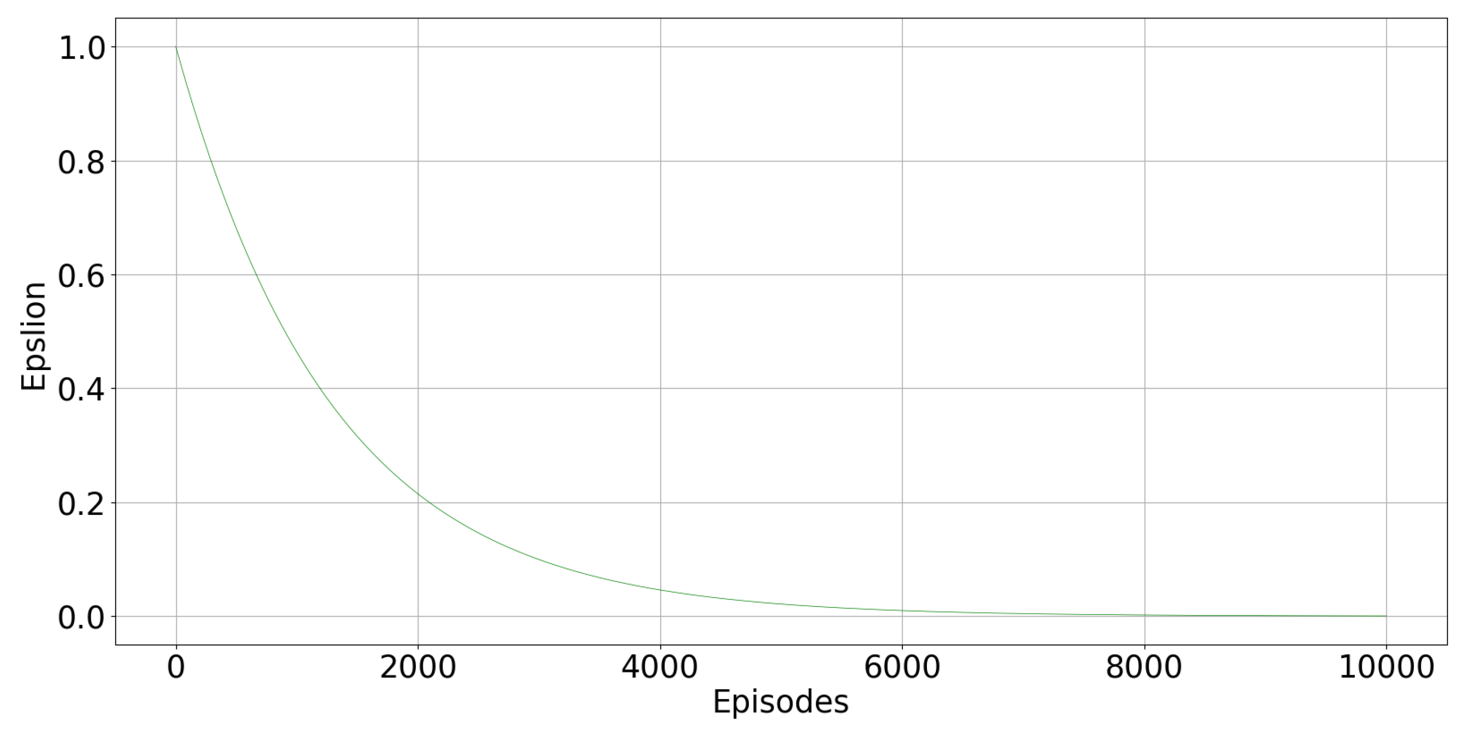
Figure 3 displays how the parameter $ϵ$ varies episode after episode, following (7). In the first episodes, high values of $ϵ$ encourage exploration. As the agent progresses in learning the optimal policy, $ϵ$ decreased to favour exploitation of the acquired knowledge.

5.2. Scenario 1

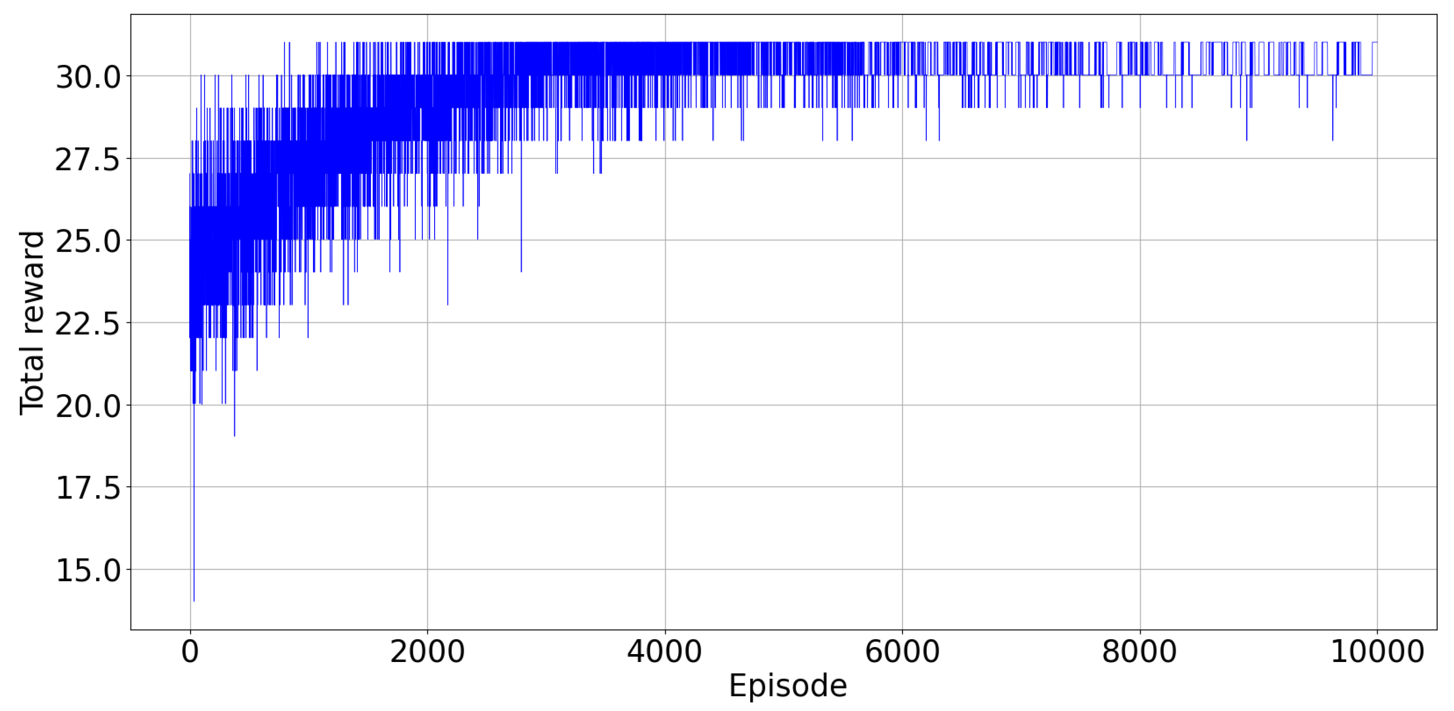
Figure 4 illustrates the total reward collected from the environment at every episode. The agents were trained over 10,000 episodes and simulation results are described below. From the Figure 4, we can empirically check that the proposed DQN algorithm converges after about 6000 episodes of training. The training process over 10,000 episodes took 2460 s.

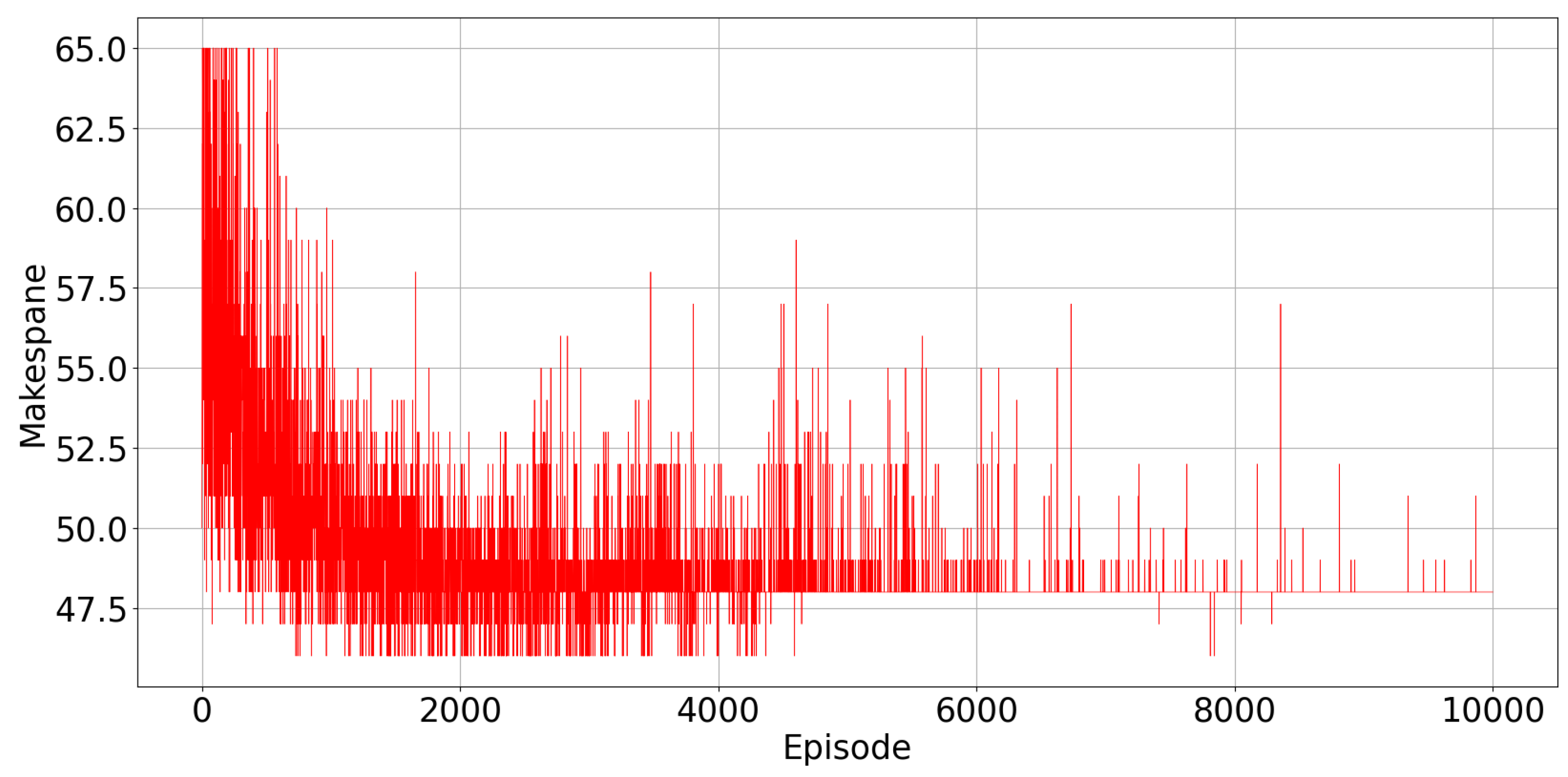
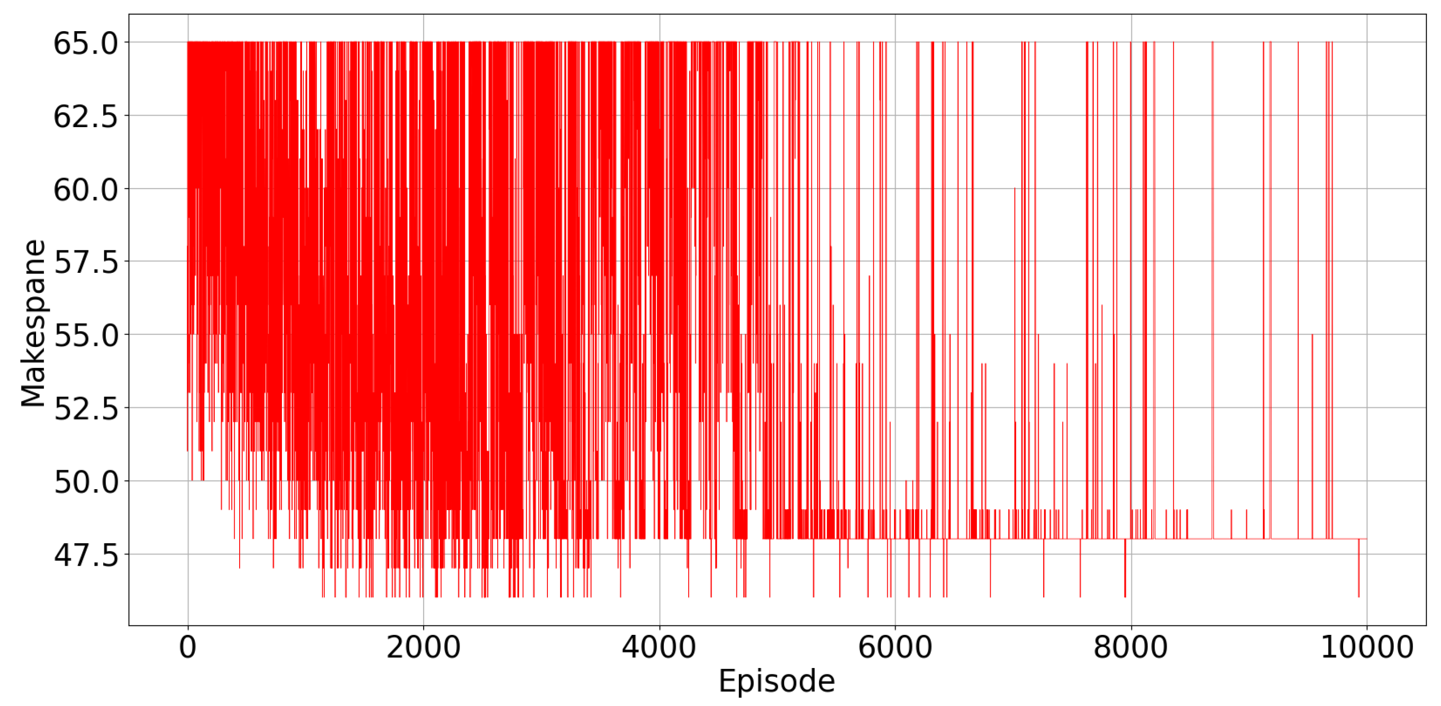
Figure 5 displays the evolution of the total make-span observed in every episode. As the learning progresses, the make-span decreases, and it converges to the minimum value of 48 time intervals. In Figure 5, there are spikes in the observed value of the make-span at some points, when the agents explore random actions. Exploration becomes less and less frequent from one episode to the other, because $ϵ$, the exploration rate, decreases, as reported in Figure 3.

We can see also from Figure 5 that in some early episodes, the observed make-span is lower than the optimal one found after learning has converged. This is because in these early episodes, the stopping criterion on the maximum possible number of iterations within a single episode is reached, and the episode is terminated before all the tasks are assigned, so that the observed make-span refers only to a portion of the total number of tasks.

The Gantt charts in Figure 6 and in Figure 7 illustrate, respectively, the placement of resources and the scheduling of tasks on workstation, as suggested by the trained agents.

It is possible to check from the Gantt charts that actually there is no alternative feasible plan of resource and task assignment that results in a lower make-span, which confirms that the agents have learned the optimal scheduling policy for the problem.

5.3. Scenario 2

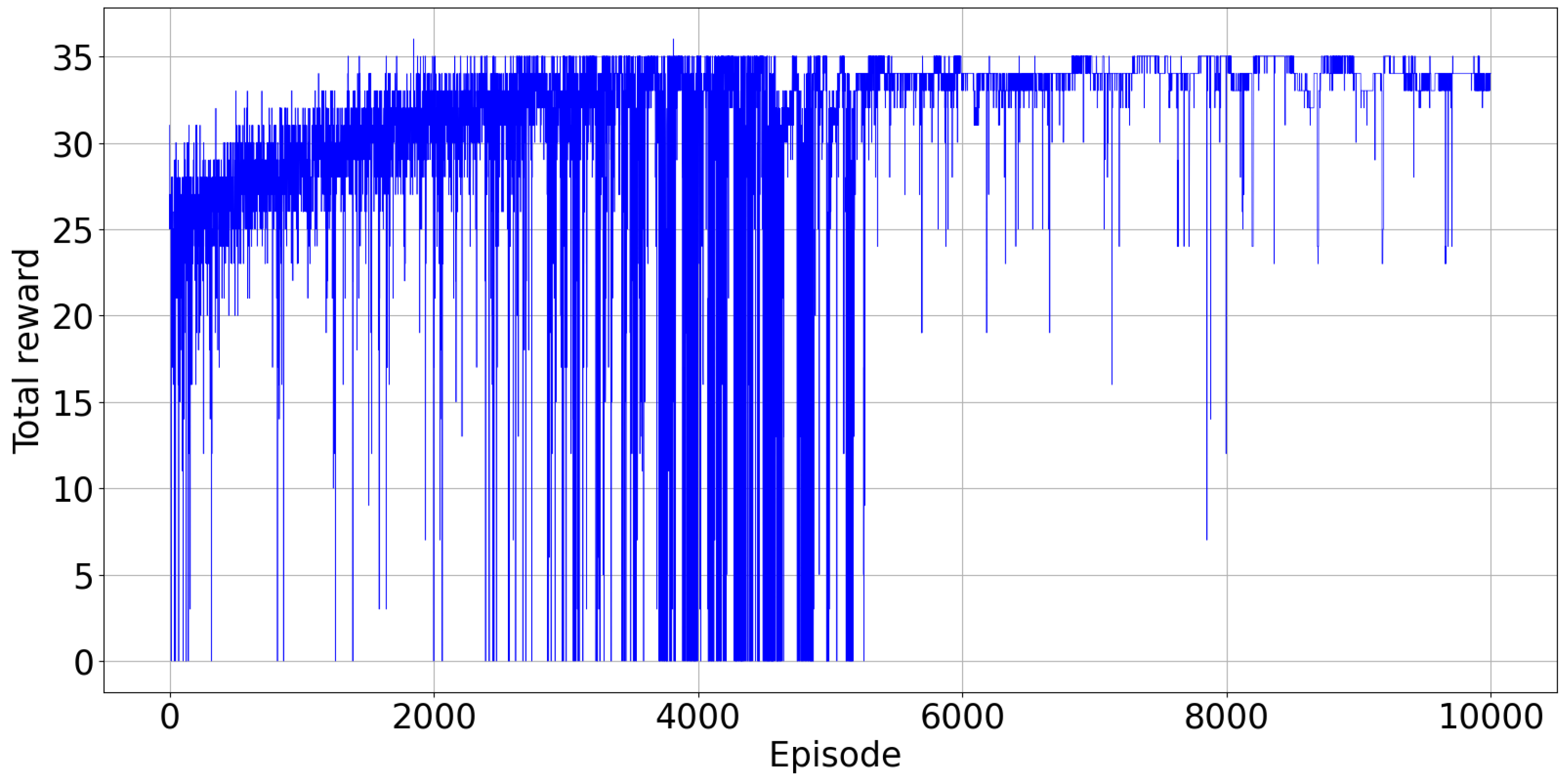
In this scenario, resource constraints are also considered, in addition to the ones already considered in Scenario 1. The agents are again trained over 10,000 episodes. Figure 8 displays the total reward collected from the environment and Figure 9 illustrates the total make-span at every episode. In Figure 9, there are again spikes in the observed value of the make-span at some points, when the agents explore random actions. Exploration becomes less and less frequent from one episode to the other, because $ϵ$, the exploration rate, decreases, as reported in Figure 3.

We can see in some early episodes that the observed make-span is again lower than the optimal one found after learning has converged, for the same reasons as above.

Figure 10 and Figure 11 report, respectively, the optimal assignment of resources and tasks to workstations.

5.4. Comparison with State-of-the-Art Approaches

We compare the proposed algorithm with a heuristic solution for task scheduling, and with an optimization-based algorithm implementing a Model Predictive Control (MPC) scheme for task control. These are two popular solutions in assembly line control. The comparison is performed based on Scenario 2 above. The main key performance indicators of interest for the comparison are:

• The total time to complete the tasks (cycle time). This gives a measure of how good the algorithm is in optimizing the tasks’ execution;
• The execution time of the algorithm. This tells us how fast the algorithm is in computing the tasks’ scheduling. This is important, especially when there is the need to update the scheduling in real time (e.g., due to faults).

5.4.1. MPC for Task Execution Control

We implemented the MPC algorithm proposed in our previous work [33], which controls the allocation of tasks and resources to the workstations in discrete time, with sampling time of T seconds. The MPC logic foresees that, every T seconds, an optimization problem is built and solved, to decide the best allocation of resources and tasks to workstations, while respecting all the applicable constraints. The target function of the MPC algorithm is designed to achieve the minimization of the cycle time. The MPC algorithm has been implemented in Julia 1.7 (https://julialang.org/, accessed on 21 December 2021), and the optimization problem solved using the solver Gurobi (https://www.gurobi.com/, accessed on 21 December 2021).

The average detected solving time of the MPC algorithm was $21.2$ s, which compares with an almost instantaneous running time ($0.046$ s) of the trained agents of the algorithm proposed in this paper. This gap is expected to be much larger in larger scenarios, with higher number of tasks, resources and workstations. Additionally, the solving time of the MPC algorithm increases further when the sampling time is decreased (in this simulation, we considered for the MPC algorithm a sampling time $T=15$ min). Due to its almost instantaneous speed, the proposed deep RL approach is more usable in real-time applications, for example, when there is the need to reschedule tasks in real time.

The total time to complete the tasks resulting from the MPC algorithm is 46 time steps (compared to a cycle time of 48 time steps resulting from the proposed RL approach).

5.4.2. Shortest Processing Time Heuristic

In the following, Scenario 2 is solved by using the Shortest Processing Time (SPT) heuristic, which is one of the heuristics often used in practice to derive simple and effective task scheduling. This heuristic gives precedence in the execution to the tasks with the shortest processing time. The assumptions used in SPT are the following ones:

• In the assignment problem, if both workstations are free, priority is given to workstations’ IDs;
• In the assignment problem, if two or more tasks have the same processing time, priority is given to tasks’ IDs.

The rule repeatedly tries to send in execution first the tasks with shortest execution time, after all the constraints are verified to be satisfied.

The heuristic has negligible computing times. Figure 12 reports the resulting tasks’ Gantt chart. The total time to complete the tasks is 52 time steps.

In conclusion, the MPC provides solutions that are characterized by the minimum total time to execute the tasks. This is achieved at the expense of the computational complexity, and the complexity of the control architecture (the approach requires to build and solve an optimization problem, and a detailed modelling of the problem). On the contrary, simple heuristics, such as the SPT one, require no computational complexity and modelling effort, at the expense of achieving a suboptimal solution, often far from the optimal one. The proposed approach presents the benefits of both the optimization-based approaches and the heuristics, being characterized by low computational complexity required to execute it in real time, low complexity of the control architecture and reduced modelling effort, and good optimization of the cycle time (achieving a value that is intermediate between the optimal one, achieved by MPC, and the one achieved by the heuristics). In conclusion, the RL approaches such as the one presented in this paper, which are made more powerful and scalable by the use of neural networks, can be integrated and can benefit from the ongoing Industry 4.0 digitalization trend (especially in the training phase, thanks to the digital twin concept), and appear as a very promising solution for making the assembly lines more agile and able to optimally react, in real time, to disruption, that could otherwise seriously impair the productivity of the factory.

6. Conclusions

This paper has discussed a deep RL-based algorithm for optimal scheduling and control of tasks’ and resources’ assignment to workstations in an assembly line. The algorithm returns an optimal schedule for the allocation of tasks and resources to workstations in the presence of constraints. The main objective is to minimize the overall cycle time, and to minimize the amount of resources circulating in the assembly line. In contrast with the standard optimization-based approaches from operational research, the proposed approach is able to learn the optimal policy during a training process, which can be run on a digital twin model of the assembly line (the simulation environment in this paper was developed by using openAI gym [18]). Furthermore, the proposed method is scalable, and after training is completed, can be used for decision support to the scheduling operators in real time, with negligible computation times. This can also prove very useful in the scenario of replanning after an adverse event, such as unexpected delays, faults, etc.

The proposed deep RL approach solves the problem of dimensionality that impairs classical, tabular RL methods (a huge number of states and actions). A parallel training approach for the agents was used, which further reduces the training times, since more than one agent simultaneously take action and learn from the environment observation. The proposed multiagent RL approach generates promising results in terms of minimization of the makespan, which demonstrates the feasibility of the proposed method.

Future work will primarily concern the introduction of more operational constraints of the tasks within the model of the complete assembly line. Then, we will work on the components of the decision-making process such as the state and the reward. The state will be extended to include additional information available within an assembly line. This information will then be used for the design of more complex reward functions that can better coordinate the activity of the agents. Therefore, different reward functions will be designed based on different performance indicators.