
LST-GCN: Long Short-Term Memory Embedded Graph Convolution Network for Traffic Flow Forecasting

Abstract
:1. Introduction
2. Related Work
2.1. Traffic Forecasting
2.2. Convolutions on Graphs
2.3. Long Short-Term Memory Network
3. Preliminaries
3.1. Traffic Networks
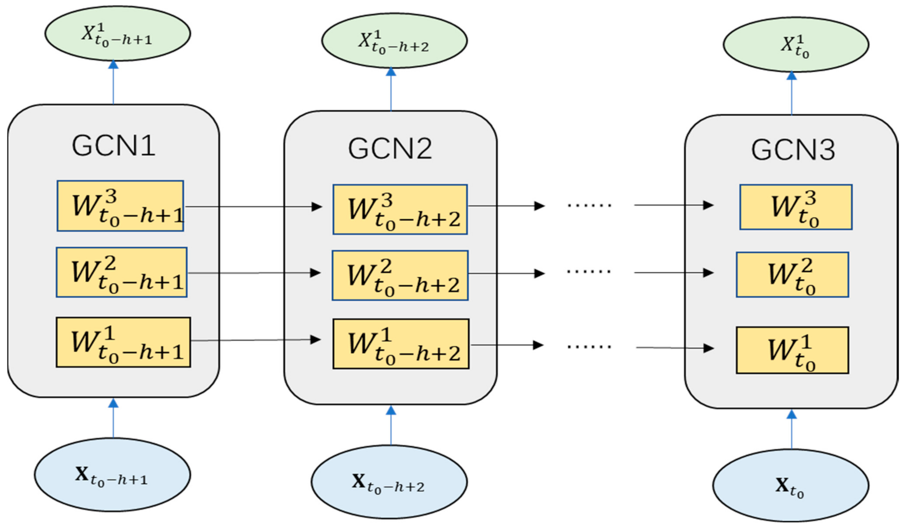
3.2. GCN Model
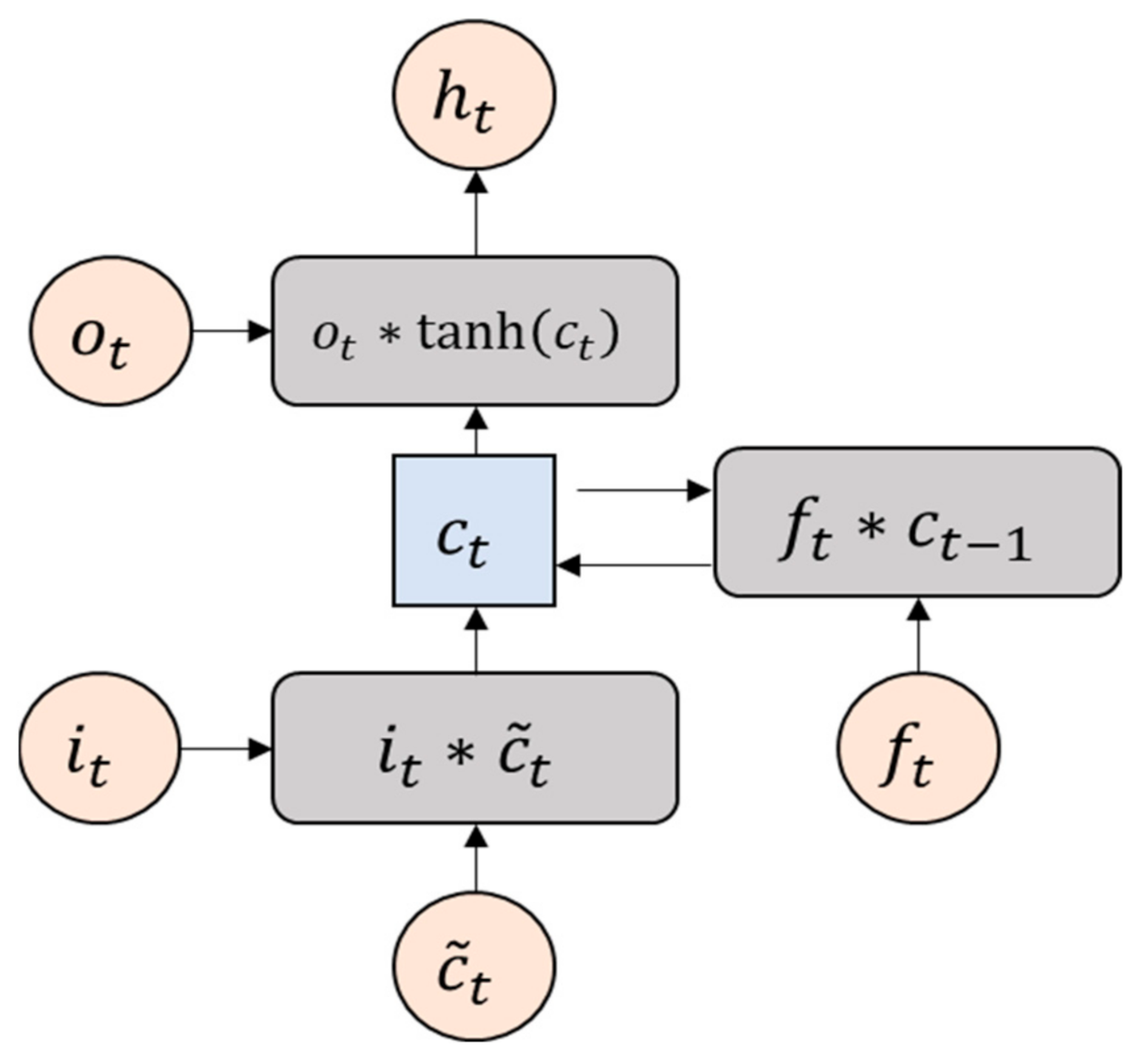
3.3. LSTM Model
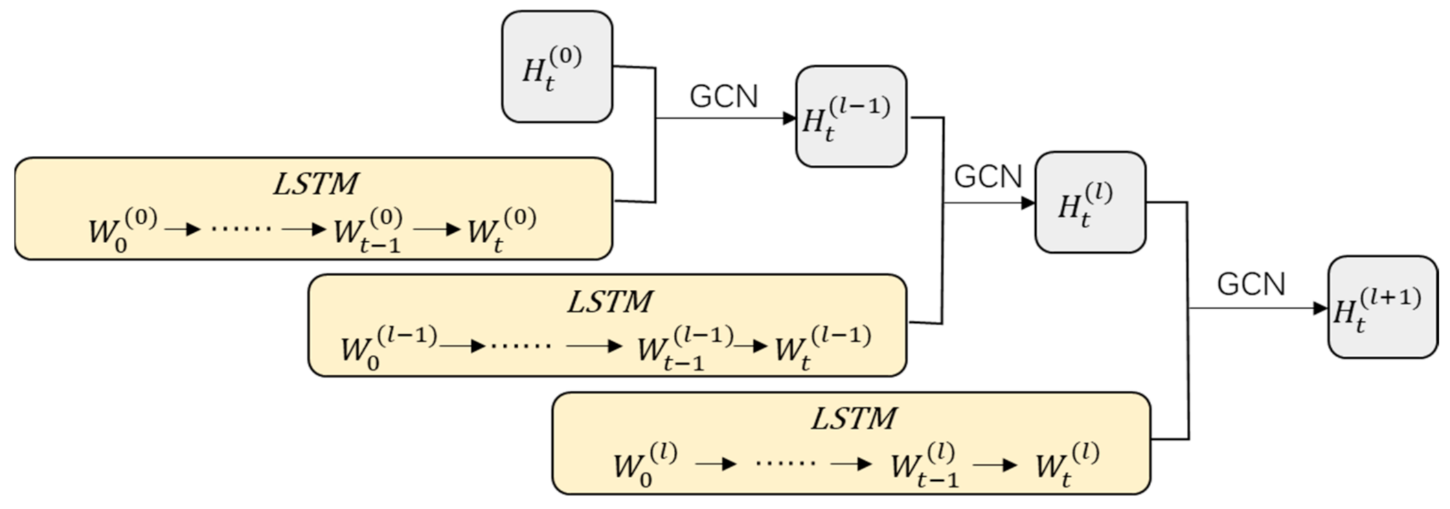
4. Method
5. Experiment
5.1. Data Set and Processing
5.2. Experimental Setup
5.3. Evaluation Indicators
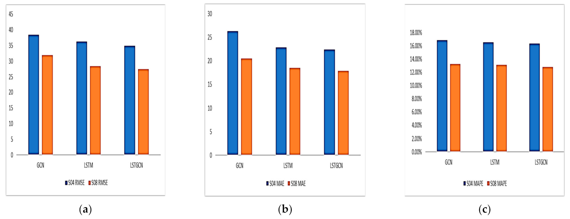
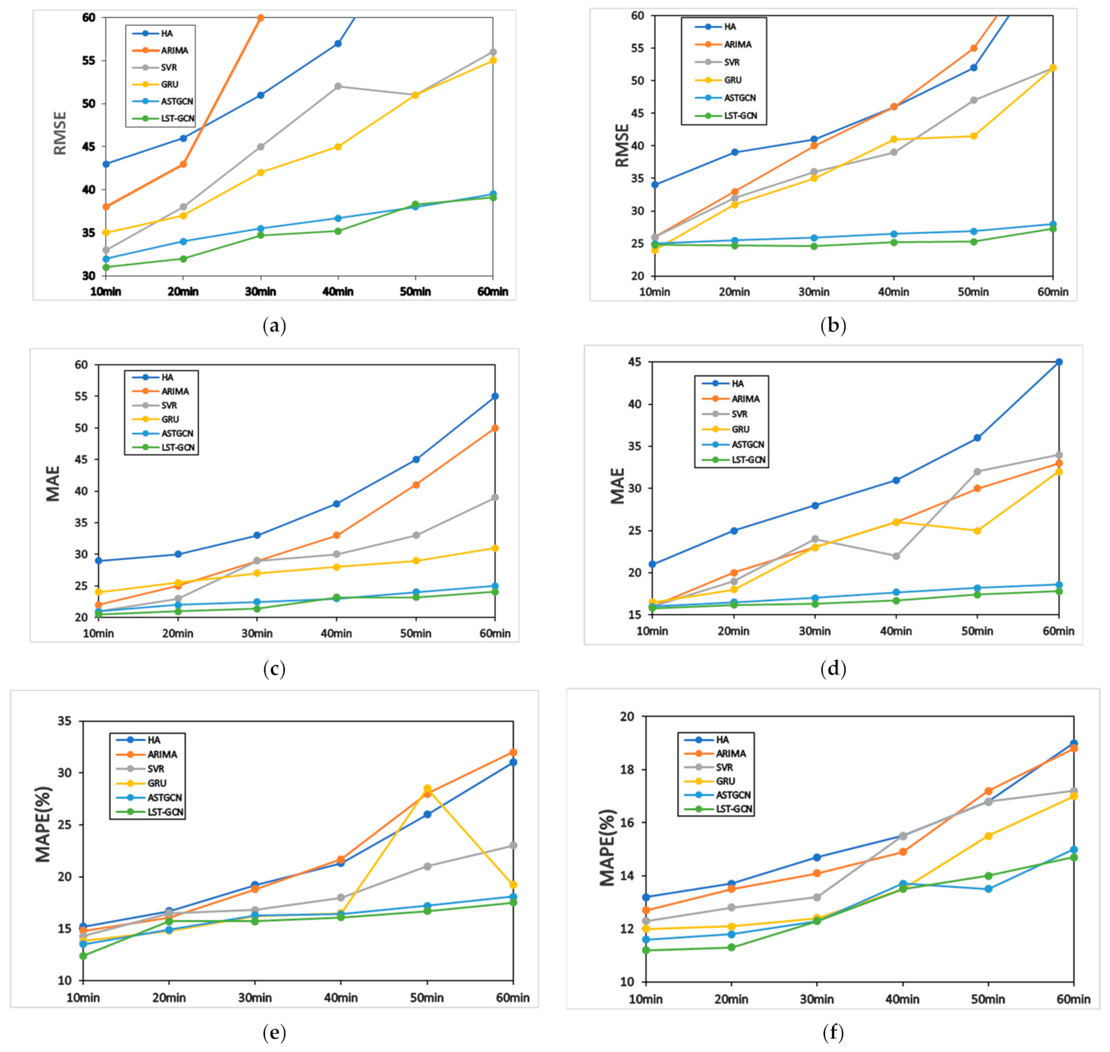
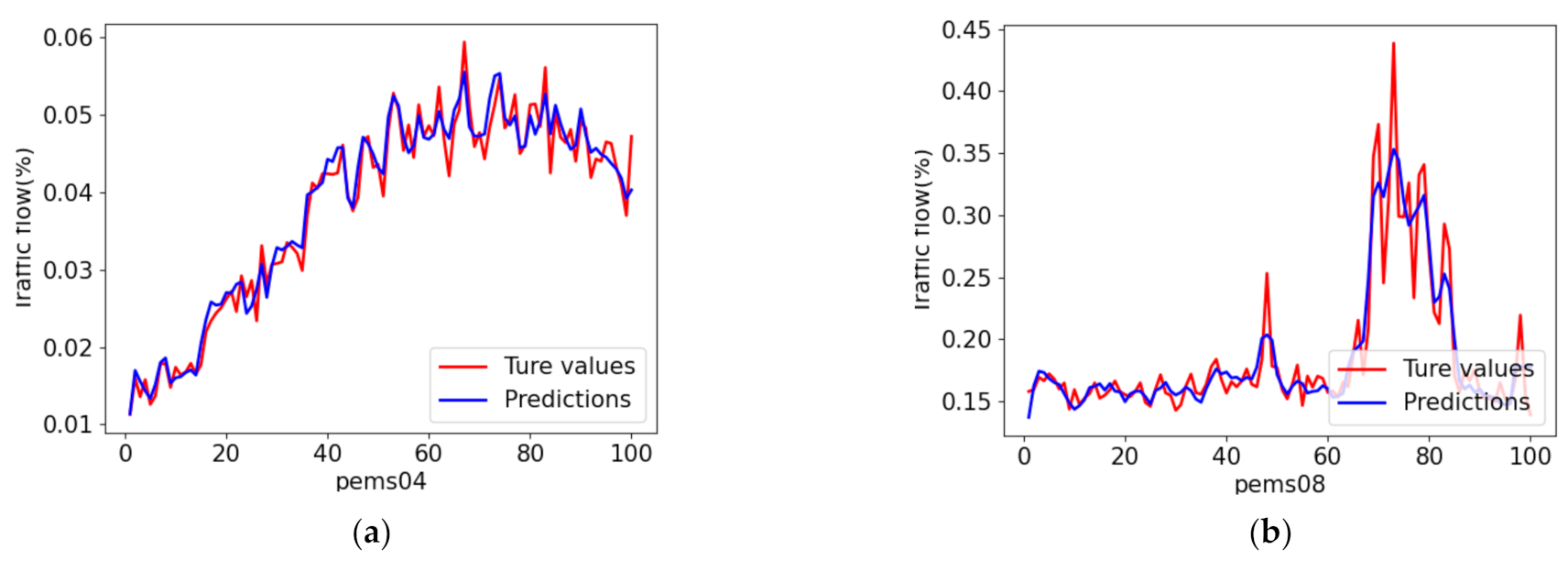
5.4. Results
6. Discussion
7. Conclusions
Author Contributions
Funding
Conflicts of Interest
Abbreviations
| GCN | Graph convolutional network |
| LSTM | Long short-term memory network |
| ARIMA | Autoregressive integrated moving average model |
| HA | History average model |
| ES | Exponential smoothing model |
| KF | Kalman filter model |
| SVR | Support vector regression model |
| KNN | K-nearest neighbor model |
| GRU | Gated recurrent unit model |
| CNN | Convolutional neural network |
| RNN | Recurrent neural network |
References
- Hani, S.M. Traveler behavior and intelligent transportation systems. Transp. Res. Part C Emerg. Technol. 1999, 7, 73–74. [Google Scholar]
- Li, Y.; Lin, Y.; Zhang, F. Research on geographic information system intelligent transportation systems. Chung-Kuo K. Lu Hsueh Pao China J. Highw. Transp. 2000, 13, 97–100. [Google Scholar]
- Liu, J.; Guan, W. A summary of traffic flow forecasting methods. J. Highw. Transp. Res. Dev. 2004, 3, 82–85. [Google Scholar]
- Ma, X.; Tao, Z.; Wang, Y. Long short-term memory neural network for traffic speed prediction using remote microwave sensor data. Transp. Res. C Emerg. Technol. 2015, 54, 187–197. [Google Scholar] [CrossRef]
- Kipf, T.N.; Welling, M. Semi-Supervised Classification with Graph Convolutional Networks. arXiv 2016, arXiv:1609.02907. [Google Scholar]
- Levin, M.; Tsao, Y.-D. On forecasting freeway occupancies and volumes. Transp. Res. Rec. 1980, 773, 47–49. [Google Scholar]
- Guo, J.; Huang, W.; Williams, B.M. Adaptive Kalman filter approach for stochastic short-term traffic flow rate prediction and uncertainty quantification. Transp. Res. C Emerg. Technol. 2014, 43, 50–64. [Google Scholar] [CrossRef]
- Shi, G.; Guo, J.; Huang, W.; Williams, B.M. Modeling seasonal heteroscedasticity in vehicular traffic condition series using a seasonal adjustment approach. J. Transp. Eng. 2014, 140, 5. [Google Scholar] [CrossRef]
- Chan, K.Y.; Dillon, T.S.; Singh, J.; Chang, E. Neural-network-based models for short-term traffic flow forecasting using a hybrid exponential smoothing and Levenberg–Marquardt algorithm. IEEE Trans. Intell. Transp. Syst. 2012, 13, 644–654. [Google Scholar] [CrossRef]
- Kumar, S.V. Traffic flow prediction using Kalman filtering technique. Procedia Eng. 2017, 187, 582. [Google Scholar] [CrossRef]
- Zhou, T.; Jiang, D.; Lin, Z.; Han, G.; Xu, X.; Qin, J. Hybrid dual Kalman filtering model for short-term traffic flow forecasting. IET Intell. Transp. Syst. 2019, 13, 1023–1032. [Google Scholar] [CrossRef]
- Cai, L.; Zhang, Z.; Yang, J.; Yu, Y.; Zhou, T.; Qin, J. A noise-immune Kalman filter for short-term traffic flow forecasting. Phys. A Stat. Mech. Appl. 2019, 536, 122601. [Google Scholar] [CrossRef]
- Zhang, S.; Song, Y.; Jiang, D.; Zhou, T.; Qin, J. Noise-identified Kalman filter for short-term traffic flow forecasting. In Proceedings of the IEEE 15th International Conference on Mobile Ad-Hoc Sensor Networks, Shenzhen, China, 11–13 December 2019; pp. 1–5. [Google Scholar]
- Castro-Netoa, M.; Jeong, Y.S.; Jeong, M.K.; Hana, L. Online-svr for short-term traffic flow prediction under typical and atypical traffic conditions. Expert Syst. Appl. 2009, 36, 6164–6173. [Google Scholar] [CrossRef]
- Chang, H.; Lee, Y.; Yoon, B.; Baek, S. Dynamic near-term traffic flow prediction: System-oriented approach based on past experiences. IET Intell. Transp. Syst. 2012, 6, 292–305. [Google Scholar] [CrossRef]
- Su, Z.; Liu, Q.; Lu, J.; Cai, Y.; Jiang, H.; Wahab, L. Short-time traffic state forecasting using adaptive neighborhood selection based on expansion strategy. IEEE Access 2018, 6, 48210–48223. [Google Scholar] [CrossRef]
- Yin, H.; Wong, S.C.; Xu, J.; Wong, C.K. Urban traffic flow prediction using a fuzzy-neural approach. Transp. Res. Part C 2002, 10, 85–98. [Google Scholar] [CrossRef]
- Çetiner, B.G.; Sari, M.; Borat, O. A Neural Network Based Traffic-Flow Prediction Model. Math. Comput. Appl. 2010, 15, 269–278. [Google Scholar] [CrossRef]
- Fu, R.; Zhang, Z.; Li, L. Using LSTM and GRU neural network methods for traffic flow prediction. In Proceedings of the 2016 31st Youth Academic Annual Conference of Chinese Association of Automation, Wuhan, China, 11–13 November 2016. [Google Scholar]
- Wu, Y.; Tan, H. Short-term traffic flow forecasting with spatial-temporal correlation in a hybrid deep learning framework. arXiv 2016, arXiv:1612.01022. [Google Scholar]
- Li, Y.; Yu, R.; Shahabi, C.; Liu, Y. Diffusion convolutional recurrent neural network: Data-driven traffic forecasting. In Proceedings of the 6th International Conference on Learning Representations (ICLR), Vancouver, BC, Canada, 30 Apr–3 May 3 2018. [Google Scholar]
- Sun, S.; Wu, H.; Xiang, L. City-Wide Traffic Flow Forecasting Using a Deep Convolutional Neural Network. Sensors 2020, 20, 421. [Google Scholar] [CrossRef] [Green Version]
- Zhao, L.; Song, Y.; Zhang, C. T-GCN: A temporal graph convolutional network for traffic prediction. IEEE Trans. Intell. Transp. 2020, 21, 3848–3858. [Google Scholar] [CrossRef] [Green Version]
- Geng, X.; Li, Y.; Wang, L. Spatiotemporal multi-graph convolution network for ride-hailing demand forecasting. AAAI Conf. Artif. Intell. 2019, 33, 3656–3663. [Google Scholar] [CrossRef] [Green Version]
- Diao, Z.; Wang, X.; Zhang, D. Dynamic spatial-temporal graph convolutional neural networks for traffic forecasting. AAAI Conf. Artif. Intell. 2019, 33, 890–897. [Google Scholar] [CrossRef]
- Huang, R.; Huang, C.; Liu, Y. Lsgcn: Long short-term traffic prediction with graph convolutional networks. Int. Joint Conf. Artif. Intell. 2020, 2355–2361. [Google Scholar]
- Lv, M.; Hong, Z.; Chen, L. Temporal multi-graph convolutional network for traffic flow prediction. IEEE Trans. Intell. Transp. Syst. 2020, 22, 3337–3348. [Google Scholar] [CrossRef]
- Guo, S.; Lin, Y.; Feng, N.; Song, C.; Wan, H. Attention Based Spatial-Temporal Graph Convolutional Networks for Traffic Flow Forecasting. AAAI Conf. Artif. Intell. 2019, 33, 922–929. [Google Scholar] [CrossRef] [Green Version]
- Bruna, J.; Zaremba, W.; Szlam, A.; LeCun, Y. Spectral networks and locally connected networks on graphs. arXiv 2014, arXiv:1312.6203. [Google Scholar]
- Defferrard, M.; Bresson, X.; Vandergheynst, P. Convolutional neural networks on graphs with fast localized spectral filtering. In Advances in Neural Information Processing Systems; Morgan Kaufmann Publishers Inc.: San Francisco, CA, USA, 2016. [Google Scholar]
- Bengio, Y.; Simard, P.; Frasconi, P. Learning long-term dependencies with gradient descent is difficult. IEEE Trans. Neural Netw. 1994, 5, 157–166. [Google Scholar] [CrossRef]
- Mauro, M.D.; Galatro, G.; Liotta, A. Experimental Review of Neural-Based Approaches for Network Intrusion Management. IEEE Trans. Netw. Service Manag. 2020, 17, 2480–2495. [Google Scholar] [CrossRef]
- Dong, S.; Xia, Y.; Peng, T. Network Abnormal Traffic Detection Model Based on Semi-Supervised Deep Reinforcement Learning. IEEE Trans. Netw. Service Manag. 2021, 18, 4197–4212. [Google Scholar] [CrossRef]
- Pelletier, C.; Webb, G.I.; Petitjean, F. Deep Learning for the Classification of Sentinel-2 Image Time Series. In Proceedings of the IGARSS 2019, Yokohama, Japan, 31 July 2019. [Google Scholar]


| Model | PMES04 | PMES08 | ||||
|---|---|---|---|---|---|---|
| RMSE | MAE | MAPE(%) | RMSE | MAE | MAPE(%) | |
| HA | 54.16 | 36.68 | 19.69 | 44.06 | 29.46 | 15.25 |
| ARIMA | 68.16 | 32.01 | 19.17 | 43.31 | 24.05 | 14.34 |
| SVR | 45.75 | 29.45 | 17.09 | 36.98 | 23.13 | 13.81 |
| GRU | 45.16 | 28.64 | 16.27 | 35.96 | 22.25 | 13.03 |
| ASTGCN | 35.23 | 22.93 | 16.58 | 28.16 | 18.61 | 13.05 |
| LST-GCN | 34.93 | 22.43 | 16.37 | 27.47 | 17.93 | 12.81 |
Publisher’s Note: MDPI stays neutral with regard to jurisdictional claims in published maps and institutional affiliations. |
© 2022 by the authors. Licensee MDPI, Basel, Switzerland. This article is an open access article distributed under the terms and conditions of the Creative Commons Attribution (CC BY) license (https://creativecommons.org/licenses/by/4.0/).
Share and Cite
Han, X.; Gong, S. LST-GCN: Long Short-Term Memory Embedded Graph Convolution Network for Traffic Flow Forecasting. Electronics 2022, 11, 2230. https://doi.org/10.3390/electronics11142230
Han X, Gong S. LST-GCN: Long Short-Term Memory Embedded Graph Convolution Network for Traffic Flow Forecasting. Electronics. 2022; 11(14):2230. https://doi.org/10.3390/electronics11142230
Chicago/Turabian StyleHan, Xu, and Shicai Gong. 2022. "LST-GCN: Long Short-Term Memory Embedded Graph Convolution Network for Traffic Flow Forecasting" Electronics 11, no. 14: 2230. https://doi.org/10.3390/electronics11142230
APA StyleHan, X., & Gong, S. (2022). LST-GCN: Long Short-Term Memory Embedded Graph Convolution Network for Traffic Flow Forecasting. Electronics, 11(14), 2230. https://doi.org/10.3390/electronics11142230