Trajectory Prediction with Correction Mechanism for Connected and Autonomous Vehicles

Abstract

Trajectory prediction of surrounding vehicles is a critical task for connected and autonomous vehicles (CAVs), helping them to realize potential dangers in the traffic environment and make the most appropriate decisions. In a practical traffic environment, vehicles may affect each other, and the trajectories may have multi-modality and uncertainty, which makes accurate trajectory prediction a challenge. In this paper, we propose an interactive network model based on long short-term memory (LSTM) and a convolutional neural network (CNN) with a trajectory correction mechanism, using our newly proposed probability forcing method. The model learns the interactions between vehicles and corrects their trajectories during the prediction process. The output is a multimodal distribution of predicted trajectories. In the experimental evaluation of the US-101 and I-80 Next-Generation Simulation (NGSIM) real highway datasets, our proposed method outperforms other contrast methods.

1. Introduction

Connected and autonomous vehicles (CAVs) have emerged as a promising technology, attracting much attention from academia and industry. CAVs have the ability of perception and communication. On the one hand, CAVs employ a variety of sensors, such as radars, lidars, and cameras, to perceive environmental information [1]. On the other hand, they can exchange information with other entities, such as other CAVs, roadside infrastructure, cloud and edge servers [2,3]. Based on the information they perceive or receive, CAVs can drive themselves autonomously. Hence, they are considered to be important components of future intelligent transportation systems.

When CAVs drive autonomously, safety is a key concern [4]. For CAVs, trajectory prediction of surrounding pedestrians [5] and vehicles [6,7,8] is a critical task that can help them to avoid potential dangers [9,10] and make appropriate path planning [11,12], which enhances traffic safety and efficiency. However, to predict the future trajectories of vehicles on the road is a challenge. In the vehicle–infrastructure collaboration scenario shown in Figure 1, the traffic environment is highly dynamic and uncertain, and the trajectories of surrounding vehicles may change at any time. Owing to the limited sensing range of its own sensors, a CAV cannot fully understand the changes in the surrounding driving environment, and vehicle-to-vehicle and vehicle-to-environment interactions may cause hazards to occur at any time. Therefore, the CAV must obtain information such as its surrounding environment and vehicle position from roadside units (RSUs) to predict the trajectories of surrounding vehicles and make more accurate decisions.

It is difficult to accurately predict the future trajectory of a vehicle only based on its past states, such as its direction and speed. The reason for this is that road environment and surrounding vehicles also have a great influence on the behavior of the vehicle. Researchers have proposed different methods to address the problems of trajectory prediction. Traditional physics-based models [13,14] do not consider the interactions of other vehicles and the surrounding environment, and they are only able to make short-term predictions in simple scenarios. With the popularity of CAVs, the road environment has become more complex. The road environment and vehicle interactions have an increasing influence on the vehicle trajectory, and a single short-term prediction is no longer sufficient for a CAV decision system to make accurate decisions. Inspired by deep learning, researchers have used deep learning networks to perform multi-feature extraction and relationship modeling of vehicle behavior. Some existing methods learn from various factors affecting vehicle trajectories to make long-term predictions [15,16].

In order to further improve the prediction accuracy, in this paper, we consider not only the interactions between vehicles and environment, but also the correction of the predicted trajectory of a vehicle during the prediction process. An interaction network model that utilizes long short-term memory (LSTM) [17] and convolutional neural network (CNN) [18] with a correction mechanism is proposed to extract and encode the spatiotemporal dependencies between vehicles. In this model, factors including locations of surrounding vehicles, historical trajectories, time, and maneuvers of vehicle are treated as dynamic backgrounds. The proposed model enables a CAV to predict the trajectories of surrounding vehicles, and the trajectories can be corrected during the prediction process to improve the prediction accuracy. The experiments based on the publicly vehicle-infrastructure Next Generation Simulation (NGSIM) datasets [19,20] prove the effect of the our proposed model.

The contributions of this paper are summarized as follows:

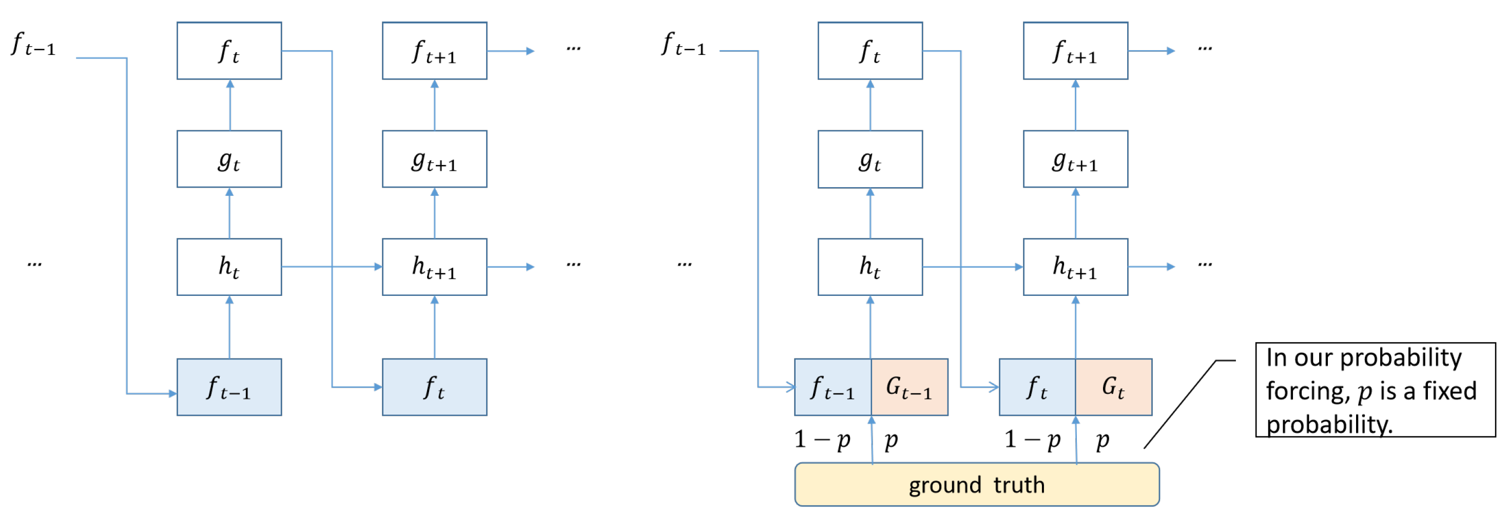
• A trajectory correction module is introduced into the interactive network model. Probability forcing is applied in the trajectory correction module to predict the trajectories of surrounding vehicles. In each step, the prediction result of the previous step or the ground truth is fed into the model with a certain probability for trajectory prediction.
• Extensive experiments are conducted based on real datasets. The prediction accuracy produced by our proposed model outperforms other recent authoritative methods in both short-term and long-term predictions, which demonstrates the effectiveness of the probability forcing scheme.

The rest of this paper is organized as follows. In Section 2, the related work on trajectory prediction, teacher forcing and scheduled sampling are summarized. The research problem is defined in Section 3, and the system model of the proposed method is established in Section 4. In Section 5, the experimental settings and the comparison models are presented. In Section 6, the experimental results are analyzed, and the potential problems are discussed. Finally, conclusions are drawn in Section 7.

2. Related Work

2.1. Trajectory Prediction

As trajectory prediction is an important task of autonomous vehicles, many methods have been proposed to solve this issue in recent years. These methods can be categorized [21,22] into three types, which are physics-based prediction, maneuver-based prediction, and interaction-aware prediction, respectively.

Physics-based prediction models [13,14] assume that the behaviors of vehicles only depend on the physical factors of their movement, including vehicle shape, acceleration, steering, and other external conditions. As only low-level motion characteristics are considered, such models are only suitable for the short-term predictions [23] (e.g., within 1 s), and cannot make long-term predictions (e.g., within 5 s) due to certain maneuvers (e.g., sudden deceleration) or interactions with surrounding vehicles (e.g., braking for the leading vehicle).

The core idea of maneuver-based prediction methods [24,25] is to classify vehicle movements into semantically interpretable maneuver classes. More specifically, Tomar et al. [24] adopt multi-layer perceptrons to predict vehicle trajectories during lane changing. Schreier et al. [25] describe an integrated Bayesian approach to make maneuver-based trajectory prediction and criticality assessment. They infer the distribution of advanced driving maneuvers for each vehicle in a traffic scenario by Bayesian inference. Subsequently, maneuver-based probabilistic trajectory prediction models are employed to predict each vehicle’s configuration forward in time. Long-term prediction [26,27] is a current hot issue. Most physics-based and maneuver-based methods do not account for interactions between vehicles, which leaves a large gap between model predictions and actual trajectories. The reality that these solutions are not suitable for long-term prediction has led to the emergence of interaction-aware methods, which consider vehicle intention and contextual information (e.g., map information and interactions between vehicles) to obtain more accurate results.

In interaction-aware methods [15,16,28], vehicles are viewed as interaction-aware mobile entities. These methods always contain a vehicle interaction module that considers the traffic environment and interactions between vehicles. Most existing studies have used interaction-aware intention and mobility prediction frameworks for complex traffic scenarios. Several studies have analyzed the effectiveness of LSTM at predicting the movement of surrounding vehicles. Inspired by the social LSTM architecture [28], many approaches have successfully migrated the method to the task of predicting vehicles. Deo and Trivedi [15] propose a convolutional social pooling method with a maneuver-class LSTM decoder, encoding and decoding multimodal predicted trajectories based on the behavior and historical trajectories between vehicles. Mersch and Hollen [29] propose a new data-driven approach to predict the motion of vehicles in a road environment, which uses a spatiotemporal convolutional network model to jointly exploit correlations in both spatial and temporal domains to capture interactions between vehicles, and predict trajectories over the next 5 seconds by considering vehicle maneuver intentions and motions. Zhao et al. [16] propose a multi-agent tensor fusion network to simulate the social interaction behaviors among vehicles on a highway, which can encode scene background images together with the trajectories of past vehicles, and use adversarial loss to improve the prediction capability for multiple vehicles. Additional methods simulate the interaction between vehicles and extract other relevant features to predict trajectory based on new tools, such as multi-headed attention [30], graph neural networks [31], etc.

2.2. Teacher Forcing and Scheduled Sampling

The predictive power of recurrent neural network (RNN) is very weak in the early stages of training iterations. The incorrect result of one step inevitably affects subsequent learning, resulting in slower learning of the model and difficulty in convergence. Teacher forcing [32,33] is proposed to solve this problem. It plays a crucial role in machine translation, contextual analysis and image captioning. Instead of using the output of the previous state as the input of the current state each time, it directly uses the corresponding term of the ground truth of the training data. However, teacher forcing has the disadvantage that children who always rely on the teacher will not progress far. Because of the reliance on labeled data, the model will work better during training, but during testing, because it cannot be supported by the ground truth, the model becomes fragile if the currently generated sequence differs significantly during training. To solve the exposure bias problem of teacher forcing in natural language processing (NLP), scheduled sampling [32,34], as shown in Figure 2. It mainly consists of three processing methods, namely linear decay, exponential decay, and inverse sigmoid decay [34]:

• Linear decay: $p_i=max(p,k-ci)$ where $0\le p<1$ is the minimum amount of truth to be given to the model, and k and c provide the offset and slope of the decay, which depend on the expected speed of convergence, i represents the number of the i-th mini-batch.
• Exponential decay: $p_i=k^i$ where $k<1$ is a constant that depends on the expected speed of convergence.
• Inverse sigmoid decay: $p_i=k/(k+exp(i/k))$ where $k\ge 1$ depends on the expected speed of convergence.

It improves performance by feeding the model a mixture of embeddings from teacher forcing and model predictions from the previous training step. Good results were achieved in the language generation model used for a transformer [35].

3. Problem Description

The present work uses the CAV to predict and correct the trajectories of surrounding vehicles. Following the same setting proposed by Deo and Trivedi [15], we discretize the space centered around the target vehicle into a 3 × 13 grid. The rows represent the current and adjacent lanes of target vehicle, and the columns represent discrete grid cells. Each surrounding vehicle is assigned a grid cell. As depicted in Figure 3, when a CAV predicts the trajectories of surrounding vehicles, in addition to their historical trajectories, we consider the interaction between vehicles and the lane changing behaviors of individual vehicles (e.g., change lane to right or left, or keep lanes). At the same time, the longitudinal behaviors of vehicles, including normal driving and braking, are also considered. Lane change behavior can be understood by the lane number where a vehicle is located. A 3 × 13 tensor is used to represent the lane changing behavior of the vehicle. When a value in the tensor is 1, the vehicle changes lanes to the corresponding lane. A vehicle is defined as performing a braking maneuver when its average speed within the predicted range is less than 0.75 times the speed at the time of prediction.

3.1. Inputs and Outputs

In this paper, we use the historical trajectories in the past $t_{obs}$ seconds to predict the trajectories in $t_{pred}$ seconds, taking as input the past trajectories of the target vehicle and its surrounding vehicles X, which is denoted as:

$$X=[{\mathbf{x}}^{t-t_{obs}},\dots ,{\mathbf{x}}^{t-1},{\mathbf{x}}^t]$$

(1)

where

$${\mathbf{x}}^t=[x_0^t,y_0^t,\dots ,x_{n-1}^t,y_{n-1}^t,x_n^t,y_n^t]$$

(2)

represents the longitudinal and lateral positions of the predicted vehicle and all surrounding vehicles at time t. The x-axis and y-axis, respectively, represent the direction of movement on the road and perpendicular to the road.

The output parameters of our model characterize a conditional probability distribution $P(Y\mid X)$, of the predicted positions of the target vehicle

$$Y=[{\mathbf{y}}^{t+1},{\mathbf{y}}^{t+2},\dots ,{\mathbf{y}}^{t+t_{pred}}]$$

(3)

where

$${\mathbf{y}}^t=[x^t,y^t]$$

(4)

denotes the predicted coordinates of the vehicle, the conditional probability distribution $P(Y\mid X)$ that can behave as a bivariate Gaussian distribution with parameters ${\theta }^t$ = (${\mu }^t,{\Sigma }^t$) at each future time step $t\in \{t+1,\dots ,t+t_{pred}\}$, where

$${\mathbf{y}}^t\sim N({\mu }^t,{\Sigma }^t),$$

(5)

where ${\mu }^t$ = $\left(\begin{array}{c}{\mu }_x^t\\ {\mu }_y^t\end{array}\right)$ is the mean vector and ${\Sigma }^t$ = $\left(\begin{array}{cc}{\left({\sigma }_x^t\right)}^2& {\sigma }_x^t{\sigma }_y^t{\rho }^t\\ {\sigma }_x^t{\sigma }_y^t{\rho }^t& {\left({\sigma }_y^t\right)}^2\end{array}\right)$ is the covariance matrix.

3.2. Probability Forcing

Although teacher forcing and scheduled sampling [32,33,34] have achieved good results in natural language processing, no application has emerged for frequency-sampled prediction. Aiming to solve the problem presented in this paper without ignoring the drawbacks of teacher forcing and scheduled sampling, a probability forcing method is proposed to solve this problem based on the ideas of these two methods, using a fixed probability to feed the prediction result of the previous step mixed with ground truth into the decoder. In order to ensure that the number of corrections is an integer, the probability is set as a product of an integer and the sampling period. It determines how many times the ground truth has been fed into the decoder. The formula is described as follows:

$$p=n\times \frac{1}{f}$$

(6)

where n is an integer that can be viewed as the number of corrections, and f represents the frequency of data sampling. The probability p is a fixed correction rate, where 0 < p < 1. The ground truth is fed into the decoder as the input with a probability of p, and the output of the previous step is used as input with a probability of $1-p$, as demonstrated in Figure 2.

4. System Model

It is crucial to understand the relationships and interactions that occur on the road to accurately predict vehicle trajectories. As shown in Figure 4, our model architecture has four main components.

4.1. Encoding Layer

The embedding module obtains the historical trajectory features of the vehicle and its neighbors, which are passed into the LSTM encoder. When trajectory correction is performed, a real vehicle trajectory at a certain moment is fed into the LSTM decoder to correct the predicted trajectories. The LSTM encoder is used to encode the evolution in vehicle trajectories and motion characteristics over time. It receives the recent $t_{obs}$ s of the CAV and the historical trajectories of all surrounding vehicles from the embedding module, whose hidden states at each time step are updated according to the hidden state of the previous time step and the input of the current time step, and whose final state can be used to encode the trajectory history and relative position information of these vehicles. Each vehicle shares LSTM weights, allowing direct correspondence between the LSTM states of all vehicles.

4.2. Convolutional Interaction Layer

As the behavior of vehicles on a road can be highly correlated, their interactions must be considered when predicting their trajectories [36], as indicated by the blue dashed line in Figure 3. When drivers decide to perform a specific motion, they shift attention to a set of surrounding vehicles in the region, as when they pay attention to the vehicles in the target lane when making a lane change. The LSTM encoder captures the motion states of vehicles, but not their interdependence in the scene. Lee et al. [37] utilized social pooling to solve this problem, pooling the LSTM states of all vehicles in the vicinity of the predicted vehicle in a social tensor by defining a spatial grid around the predicted vehicle and populating it with LSTM states based on the spatial configuration of the vehicles in the driving scenario. In the convolutional interaction layer, a modified social pooling method [15] is used to combine convolution and social pooling. The equivariance of the convolution layer helps to learn locally useful features in the social tensor space grid, while the max-pooling layer adds local translational invariance. The social tensor is created by a lane based grid, with a 13 × 3 grid region around the predicted vehicle, where each column corresponds to a lane, each row is spaced about the length of a vehicle, and the social tensor is formed by populating this grid with the surrounding vehicle locations. Two convolutional layers and a pooling layer are then applied to the social tensor to obtain a social environment code. In addition, the LSTM state of the predicted vehicle is passed through a fully connected layer to obtain the vehicle dynamics encoding, and the two encodings are connected to form a complete trajectory encoding that is passed to the decoding layer.

4.3. Trajectory Correction Module

Previous works [15,16,29] consider various factors in vehicle interactions, but they do not consider correcting the trajectories of the prediction process in a vehicle–infrastructure collaboration scenario to achieve a more accurate result. In the trajectory-correction module, we correct the predicted trajectory using probability forcing, obtaining the ground truth at a certain moment from the embedding module and feeding it to the LSTM decoder with probability p (an integer multiple of the sampling period). Instead of using the prediction result of the previous step as the input of the next step, we performed this according to the mixture between the ground truth and the model prediction. The correction module is connected to the embedding module and the decoding layer. When correction is needed, it obtains information such as the true position of the current step from the embedding module to pass to the decoder. Through the final process, the predicted decoder performs back-propagation. The performance of this module is discussed further in Section 6.2.

4.4. Decoding Layer

Owing to the complexity of traffic scenes and differences in driving styles, vehicles have uncertain driving trajectories. We use the LSTM-based decoder, combined with the classification of future lane change intentions of vehicles in Figure 3, to generate a binary Gaussian distribution of future $t_{pred}$ s, to obtain the predicted distribution of vehicle trajectories. The decoder feeds back the decoding result to the correction module, which controls the feeding of the real value to realize the correction of the trajectories.

5. Experimental Evaluation

5.1. Experimental Settings

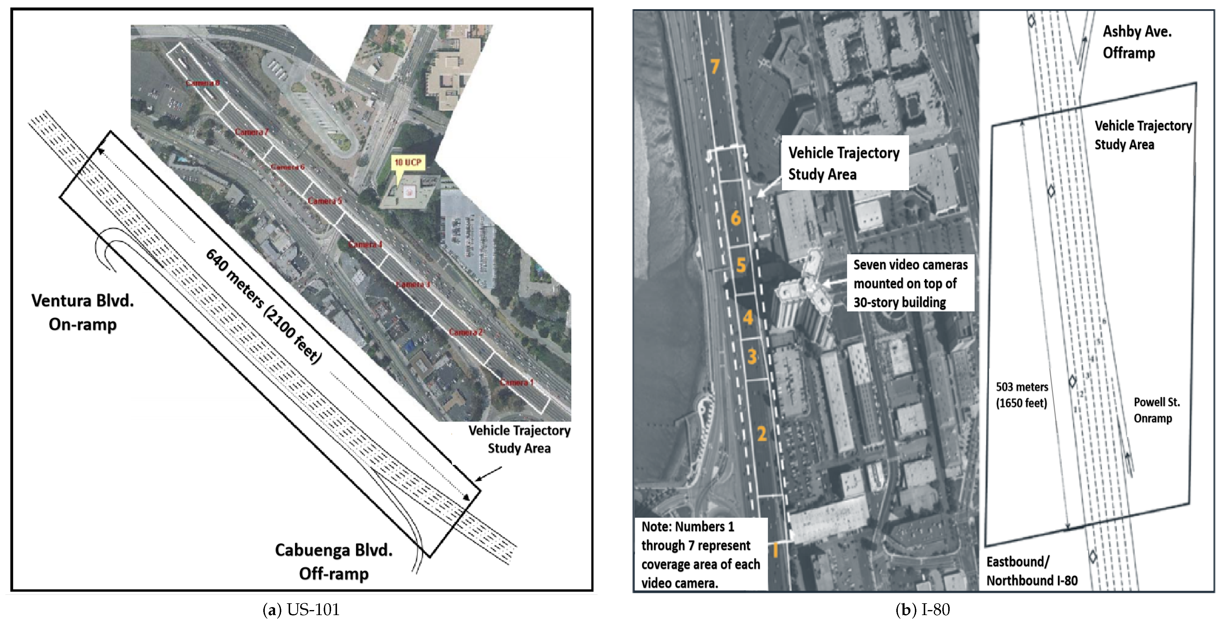
Our model is fully differentiable and can be trained end-to-end by minimizing the mean square error (MSE) [38] loss,

$$Los{s}_{MSE}=\frac{1}{t_{pred}}\sum _{pred=t+1}^{t+t_{pred}}{(x_{pred}-x)}^2+{(y_{pred}-y)}^2$$

(7)

We train the model using the Adam [39] optimizer with the hyper-parameters set in

Table 1. The hyper-parameters setting of the Adam optimizer and model network.

Hyper-Parameter	Value
learning rate	0.001
${\beta }_1$	0.9
${\beta }_2$	0.98
$ϵ$	${10}^{-9}$
batch_size	128
encoder_size	64
conv1_depth	64
conv2_depth	16
decoder_size	128
activation function	leaky-ReLU ($\alpha$ = 0.1)

. The LSTM encoder has a 64-dimensional state, and the decoder has a 128-dimensional state. The convolutional interaction module learns spatial dependencies between vehicles, with convolutional layers of 64 and 16 dimensions, and a maximum pooling layer. The size of fully connected layer for obtaining vehicle dynamics encoding is 32. Leaky-ReLU is as activation with $\alpha =0.1$ for all layers. The model is implemented on PyTorch, and it runs on a computer with Intel Core i9 9900 CPU, 64G memory and RTX 2080 GPU.

5.2. Datasets

Our experiments used the NGSIM public dataset, which is suitable for vehicle–infrastructure collaboration studies, and consists of two subsets, US-101 [19] and I-80 [20], of trajectories of real highway traffic captured at 10 Hz, and the scenario layout of its acquisition dataset is shown in Figure 5. Each subset consists of three 15 min segments recorded over a span of 45 min. The road section consists of five lanes, whose traffic conditions were recorded. The datasets provided the longitudinal and lateral coordinates of vehicles projected to a local coordinate system, in addition to data such as vehicle number, vehicle class, lane number, velocity, and acceleration. We divided these two subsets into training (70%), validation (10%) and testing (20%) sets, and extract the necessary data as input to the model. The vehicle trajectories are segmented into 8 s segments. We use the historical trajectories with $t_{obs}$ = 3 s to predict the trajectories with $t_{pred}$ = 5 s, downsampling at 5 Hz to reduce model complexity [15].

5.3. Evaluation Metric

The root mean square error (RMSE) [38], which is calculated as

$$RMSE=\sqrt{\frac{1}{t_{pred}}\sum _{i=t+1}^{t+t_{pred}}{(x_i-x)}^2+{(y_i-y)}^2}$$

(8)

is employed as the evaluation metric in trajectory prediction, reflecting the average distance deviation between the predicted and true trajectory, i.e., ($x_i$, $y_i$) and (x, y), respectively, denoting the predicted and actual horizontal and vertical coordinates at the current moment.

5.4. Comparison Models

In order to make a fair comparison, we evaluated all models on the same test set. We report the RMSE for each prediction step, which is a common evaluation metric in trajectory-prediction tasks. Using the proposed model and the following comparison models:

• CS-LSTM(M) [15]: This convolutional social pooling approach with a maneuver class LSTM decoder generates multimodal trajectory predictions based on two longitudinal and three lateral behaviors;
• MATF [16]: This model encodes the scene context and past vehicle trajectories, and deploys convolutional layers to capture interactions. The decoder generates predicted trajectories using adversarial loss;
• NLS-LSTM [40]: Local and non-local operations are combined to generate an adapted context vector for social pooling. The non-local multi-head attention mechanism captures the relative importance of each vehicle and the local blocks represent nearby interactions between vehicles;
• JSTM [41]: This joint time-series model is based on the shared LSTM layer and further FC regression networks for different driving styles. A common LSTM temporal pattern network is trained, and concatenate networks are fine-tuned for each driving style;
• PiP [42]: a planning-coupled module extracts interaction features with a special channel for injecting future planning, and a target fusion module encodes and decodes tightly coupled future interactions among agents;
• MTP [29]: a spatiotemporal convolutional network model captures interactions between vehicles to predict trajectories considering multiple possible maneuvering intentions and movements of vehicles.

6. Results and Discussion

6.1. Results

The above comparison models all consider the interaction between vehicles, but the processing of vehicle interactions and the inputs of the background are different. They are given the historical trajectories and other dynamic background information (e.g., vehicle interaction vectors and scene context vectors) of the target and surrounding vehicles, and output probability distributions on the future trajectory of the target vehicle.

Table 2. Comparison of RMSE at each prediction horizon evaluated on NGSIM datasets. Bolded numbers indicate best results.

Datasets	Prediction Horizon(s)	CS-LSTM(M)	MATF	NLS-LSTM	JSTM	PiP	MTP	Ours
	1	0.62	0.66	0.56	0.57	0.55	0.53	0.45
	2	1.29	1.34	1.22	1.38	1.18	1.17	0.98
NGSIM	3	2.13	2.08	2.02	2.21	1.94	1.93	1.72
	4	3.20	2.97	3.03	3.03	2.88	2.88	2.78
	5	4.52	4.13	4.31	3.77	4.04	4.05	4.26

shows RMSE values for the models being compared on the NGSIM datasets. The evaluation results show that the longer the prediction time the larger the model error. At the same time, from the perspective of the RMSE performance of each model, there are certain differences in performance due to different modeling of vehicle interactions and background factors considered. Our method significantly outperformed the other methods in the range of 1 s to 4 s. Compared to the best-performing method (i.e., MTP), our method reduced the prediction error by 15.1% within 1 s, by 10.9% within 3 s, and by 3.5% within 4 s. However, at 5 s, our method only outperforms CS-LSTM(M) [15] and NLS-LSTM [40], and is inferior to the other comparison methods. The possible reason for this is that our method is based on the improvement of CS-LSTM(M) [15], and the factors affecting vehicle trajectory are not sufficiently considered, thus its performance is lower than other methods in longer-term predictions. However, the experimental results prove that our trajectory correction is effective.

To further validate the advantages of our proposed model, we selected several other methods applied in short-term forecasting. The first one is a simple physics-based model that predicts the trajectory of the target vehicle from longitudinal and lateral velocities and historical trajectories. The second one is SA-LSTM [43], an LSTM model with only spatial attention mechanism, which selects the last hidden state containing the latest trajectory information to form a spatial attention layer, and fuses the information of the target vehicle and nearby vehicles to predict the trajectory. The third one is CS-LSTM [15], which is compared to above-mentioned CL-LSTM(M); CS-LSTM does not consider the influence of the vehicle’s maneuver on the trajectory. The last one is the state-of-the-art short-term prediction method STA-LSTM [44], which predicts vehicle trajectories within 1 s using an interpretable spatiotemporal attention mechanism. The results in Figure 6 show that the physics-based model performs the worst of all the models compared within five time steps (each time step is 0.2 s), also indicating that the traditional physics-based model is no longer advantageous in today’s vehicle trajectory prediction. Our method that utilizes trajectory correction shows a tremendous improvement in performance over the physics-based model within five time steps (each time step is 0.2 s). There is also a significant advantage over the state-of-the-art equivalent model. These results are sufficient to illustrate the short-term forecasting performance of our method.

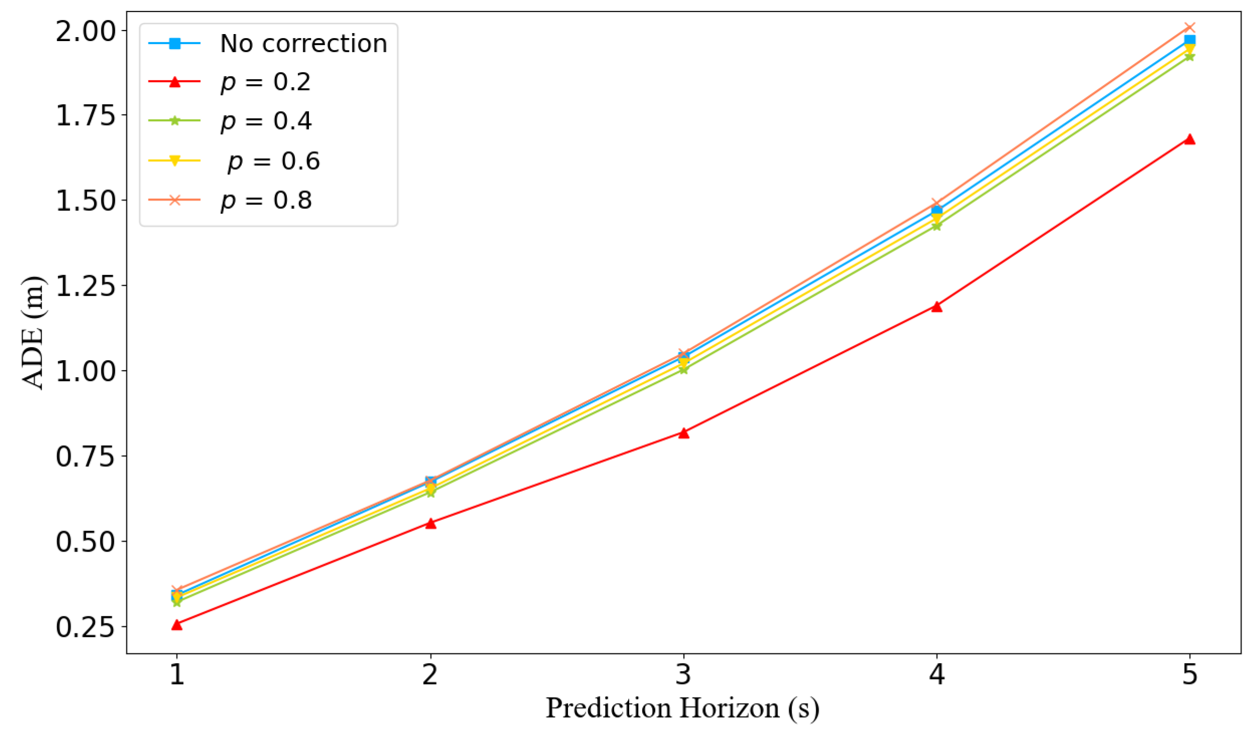
6.2. Analyzing the Correction Module in Trajectory Prediction

This module can learn how to correct the predicted trajectory during training. We conducted experiments to evaluate whether to add the correction module and the effect of different correction rates on the prediction accuracy.

When applying the correction module, we correct the predicted trajectories with different correction rates p (0 < p < 1). In Section 3.2, we proposed probability forcing with an integer multiple of the sampling period as the correction rate when selecting it. We processed the NGSIM datasets with a sampling period of 0.2 s at each step. Therefore, we used a correction rate p that was an integer multiple of 0.2. Starting from p = 0.2, we conducted experiments separately and compared the average displacement error (ADE) [45], which is calculated as:

$$ADE=\frac{{\sum }_i^N{\sum }_{i_{t+1}}^{i_{t+t_{pred}}}\sqrt{{(x_{i_t}-x_i)}^2+{(y_{i_t}-y_i)}^2}}{N\times t_{pred}}$$

(9)

where N represents the number of vehicles; ($x_{i_t}$, $y_{i_t}$) are the predicted and actual positions, respectively, of vehicle i at time t; and $t_{pred}$ represents the prediction range.

Figure 7 shows the ADE performance for different correction rates without applying and after applying correction module. The results show that the correction module is effective. When the correction rate p = 0.2, it can also be understood that it is corrected once within 1 s, and the performance is much better than the other experiments in the prediction range. Especially at 1 s and 3 s, the ADE is reduced by 24.7% and 21.2%, respectively, compared with no correction method. When p = 0.4, the ADE performance at 2 s is the best, which is 2.7% less than no correction method. When p = 0.6, the performance is also better than when the correction module is not used, and the best performance in the predicted range is also obtained at 2 s, with a 2.2% improvement. However, at p = 0.8, it is weaker, and only when 0.2 is better than without correction. We speculate that this is due to an overcorrection. It can be seen from Figure 7 that the performance does not always improve with the improvement of the correction rate, and it also shows that it is not true that the more times the trajectory is corrected, the better the ADE performance will be. By analyzing the experimental results, it can be concluded that the correction is necessary when predicting the vehicle trajectory, but an appropriate number of corrections is needed in the prediction range.

6.3. Discussion

In Section 6.1 and Section 6.2, we analyze the experimental results and the effectiveness of the correction module in trajectory prediction, respectively. Although our method achieves competitive results, there are still limitations and potential problems. In longer-term predictions, our method performs weaker than other comparison methods, and we believe that there is insufficient consideration in handling the interactions between vehicles and the dynamic context factors where vehicles are located. Pedestrians are also present on urban roads, but our model only considers the interactions between vehicles, which may lead to inaccurate trajectory prediction in other traffic scenarios involving pedestrians. Our trajectory correction is a random correction with a fixed probability. Although the correction achieves certain effect, but when the correction rate is too large, that is, when the number of corrections is too many, the effect of overcorrection tends to occur, thus our correction mechanism can be further optimized. These issues will be focused on in our future work.

7. Conclusions and Future Work

We proposed a vehicle trajectory prediction model based on LSTM and CNN networks with a correction mechanism. The model encodes the temporal and spatial interdependencies between vehicles, combines their lane change intentions, and finally obtains the multimodal trajectory distribution of future movements of surrounding vehicles by an LSTM decoder. One of the correction mechanisms applies our newly proposed probability forcing method. It can be used to simulate CAV to obtain perceptual information from RSUs in the form of fixed probability to correct predicted trajectories. Experimental results demonstrate the effectiveness of the probability forcing approach in the trajectory correction module. It is also shown that our proposed model outperforms similar existing methods on the NGSIM dataset.

In future work, due to the potential problems of this study, we will consider the effects of factors such as pedestrians and traffic rules on vehicles trajectories, and use these factors as inputs to the model for prediction. When the trajectory is corrected, a dynamic correction mechanism will be established within the prediction range, which can dynamically determine the number of corrections and reduce the occurrence of overcorrection.

References

1. Liu, Y.; Tight, M.; Sun, Q.; Kang, R. A systematic review: Road infrastructure requirement for connected and autonomous vehicles (CAVs). In Proceedings of the Journal of Physics: Conference Series; IOP Publishing: Bristol, UK, 2019; Volume 1187, p. 042073. [Google Scholar]
2. Guanetti, J.; Kim, Y.; Borrelli, F. Control of connected and automated vehicles: State of the art and future challenges. Annu. Rev. Control 2018, 45, 18–40. [Google Scholar] [CrossRef] [Green Version]
3. Shiwakoti, N.; Stasinopoulos, P.; Fedele, F. Investigating the state of connected and autonomous vehicles: A literature review. Transp. Res. Procedia 2020, 48, 870–882. [Google Scholar] [CrossRef]
4. Bila, C.; Sivrikaya, F.; Khan, M.A.; Albayrak, S. Vehicles of the future: A survey of research on safety issues. IEEE Trans. Intell. Transp. Syst. 2016, 18, 1046–1065. [Google Scholar] [CrossRef]
5. Giuliari, F.; Hasan, I.; Cristani, M.; Galasso, F. Transformer networks for trajectory forecasting. In Proceedings of the 25th International Conference on Pattern Recognition (ICPR), Milan, Italy, 10–15 January 2021; pp. 10335–10342. [Google Scholar] [CrossRef]
6. Liu, Y.; Zhang, J.; Fang, L.; Jiang, Q.; Zhou, B. Multimodal motion prediction with stacked transformers. In Proceedings of the 2021 IEEE/CVF Conference on Computer Vision and Pattern Recognition (CVPR), Nashville, TN, USA, 20–25 June 2021; pp. 7573–7582. [Google Scholar] [CrossRef]
7. Schlechtriemen, J.; Wirthmueller, F.; Wedel, A.; Breuel, G.; Kuhnert, K.D. When will it change the lane? A probabilistic regression approach for rarely occurring events. In Proceedings of the 2015 IEEE Intelligent Vehicles Symposium (IV), Seoul, Korea, 28 June–1 July 2015; pp. 1373–1379. [Google Scholar] [CrossRef]
8. Deo, N.; Trivedi, M.M. Multi-modal trajectory prediction of surrounding vehicles with maneuver based LSTMs. In Proceedings of the 2018 IEEE Intelligent Vehicles Symposium (IV), Suzhou, China, 26–30 June 2018; pp. 1179–1184. [Google Scholar] [CrossRef] [Green Version]
9. Li, G.; Yang, Y.; Zhang, T.; Qu, X.; Cao, D.; Cheng, B.; Li, K. Risk assessment based collision avoidance decision-making for autonomous vehicles in multi-scenarios. Transp. Res. Part C Emerg. Technol. 2021, 122, 102820. [Google Scholar] [CrossRef]
10. Li, A.; Sun, L.; Zhan, W.; Tomizuka, M.; Chen, M. Prediction-based reachability for collision avoidance in autonomous driving. In Proceedings of the 2021 IEEE International Conference on Robotics and Automation (ICRA), Xi’an, China, 30 May–5 June 2021; pp. 7908–7914. [Google Scholar] [CrossRef]
11. Huang, C.; Huang, H.; Hang, P.; Gao, H.; Wu, J.; Huang, Z.; Lv, C. Personalized trajectory planning and control of lane-change maneuvers for autonomous driving. IEEE Trans. Veh. Technol. 2021, 70, 5511–5523. [Google Scholar] [CrossRef]
12. Zhao, W.; Liu, R.; Ngoduy, D. A bilevel programming model for autonomous intersection control and trajectory planning. Transp. A Transp. Sci. 2019, 17, 34–58. [Google Scholar] [CrossRef]
13. Toledo-Moreo, R.; Zamora-Izquierdo, M.A. IMM-based lane-change prediction in highways With low-cost GPS/INS. IEEE Trans. Intell. Transp. Syst. 2009, 10, 180–185. [Google Scholar] [CrossRef] [Green Version]
14. Barth, A.; Franke, U. Where will the oncoming vehicle be the next second? In Proceedings of the 2008 IEEE Intelligent Vehicles Symposium, Eindhoven, The Netherlands, 4–6 June 2008; pp. 1068–1073. [Google Scholar] [CrossRef]
15. Deo, N.; Trivedi, M.M. Convolutional social pooling for vehicle trajectory prediction. In Proceedings of the 2018 IEEE/CVF Conference on Computer Vision and Pattern Recognition Workshops (CVPRW), Salt Lake City, UT, USA, 18–22 June 2018; pp. 1468–1476. [Google Scholar] [CrossRef] [Green Version]
16. Zhao, T.; Xu, Y.; Monfort, M.; Choi, W.; Baker, C.; Zhao, Y.; Wang, Y.; Wu, Y.N. Multi-agent tensor fusion for contextual trajectory prediction. In Proceedings of the 2019 IEEE/CVF Conference on Computer Vision and Pattern Recognition (CVPR), Long Beach, CA, USA, 15–20 June 2019; pp. 12118–12126. [Google Scholar] [CrossRef] [Green Version]
17. Hochreiter, S.; Schmidhuber, J. Long short-term memory. Neural Comput. 1997, 9, 1735–1780. [Google Scholar] [CrossRef] [PubMed]
18. LeCun, Y.; Bottou, L.; Bengio, Y.; Haffner, P. Gradient-based learning applied to document recognition. Proc. IEEE 1998, 86, 2278–2324. [Google Scholar] [CrossRef] [Green Version]
19. Colyar, J.; Halkia, J. US Highway 101 Dataset; Federal Highway Administration, US Department of Transportation: Washington, DC, USA, 2007. Available online: https://rosap.ntl.bts.gov/view/dot/38724 (accessed on 20 April 2022).
20. Halkia, J.; Colyar, J. Interstate 80 Freeway Dataset; Federal Highway Administration, US Department of Transportation: Washington, DC, USA, 2006. Available online: https://rosap.ntl.bts.gov/view/dot/38708 (accessed on 20 April 2022).
21. Lefèvre, S.; Vasquez, D.; Laugier, C. A survey on motion prediction and risk assessment for intelligent vehicles. ROBOMECH J. 2014, 1, 1–14. [Google Scholar] [CrossRef] [Green Version]
22. Xie, G.; Gao, H.; Qian, L.; Huang, B.; Li, K.; Wang, J. Vehicle trajectory prediction by integrating physics- and maneuver-based approaches using interactive multiple models. IEEE Trans. Ind. Electron. 2018, 65, 5999–6008. [Google Scholar] [CrossRef]
23. Batz, T.; Watson, K.; Beyerer, J. Recognition of dangerous situations within a cooperative group of vehicles. In Proceedings of the 2009 IEEE Intelligent Vehicles Symposium, Xi’an, China, 3–5 June 2009; pp. 907–912. [Google Scholar] [CrossRef]
24. Tomar, R.S.; Verma, S. Safety of lane change maneuver through a priori prediction of trajectory using neural networks. Netw. Protoc. Algorithms 2012, 4, 4–21. [Google Scholar] [CrossRef]
25. Schreier, M.; Willert, V.; Adamy, J. An integrated approach to maneuver-based trajectory prediction and criticality assessment in arbitrary road environments. IEEE Trans. Intell. Transp. Syst. 2016, 17, 2751–2766. [Google Scholar] [CrossRef]
26. Xing, Y.; Lv, C.; Wang, H.; Cao, D.; Velenis, E.; Wang, F.Y. Driver activity recognition for intelligent vehicles: A deep learning approach. IEEE Trans. Veh. Technol. 2019, 68, 5379–5390. [Google Scholar] [CrossRef] [Green Version]
27. Mukherjee, S.; Wang, S.; Wallace, A. Interacting vehicle trajectory prediction with convolutional recurrent neural networks. In Proceedings of the 2020 IEEE International Conference on Robotics and Automation (ICRA), Paris, France, 31 May–4 June 2020; pp. 4336–4342. [Google Scholar] [CrossRef]
28. Alahi, A.; Goel, K.; Ramanathan, V.; Robicquet, A.; Fei-Fei, L.; Savarese, S. Social LSTM: Human trajectory prediction in crowded spaces. In Proceedings of the 2016 IEEE Conference on Computer Vision and Pattern Recognition (CVPR), Las Vegas, NV, USA, 27–30 June 2016; pp. 961–971. [Google Scholar] [CrossRef] [Green Version]
29. Mersch, B.; Höllen, T.; Zhao, K.; Stachniss, C.; Roscher, R. Maneuver-based trajectory prediction for self-driving cars using spatio-temporal convolutional networks. In Proceedings of the 2021 IEEE/RSJ International Conference on Intelligent Robots and Systems (IROS), Prague, Czech Republic, 27 September–1 October 2021; pp. 4888–4895. [Google Scholar]
30. Vaswani, A.; Shazeer, N.; Parmar, N.; Uszkoreit, J.; Jones, L.; Gomez, A.N.; Kaiser, Ł.; Polosukhin, I. Attention is all you need. In Proceedings of the 31st International Conference on Neural Information Processing Systems (NIPS), Long Beach, CA, USA, 4–9 December 2017; pp. 6000–6010. [Google Scholar]
31. Wu, Z.; Pan, S.; Chen, F.; Long, G.; Zhang, C.; Yu, P.S. A comprehensive survey on graph neural networks. IEEE Trans. Neural Netw. Learn. Syst. 2021, 32, 4–24. [Google Scholar] [CrossRef] [PubMed] [Green Version]
32. Drossos, K.; Gharib, S.; Magron, P.; Virtanen, T. Language modelling for sound event detection with teacher forcing and scheduled sampling. In Proceedings of the International Workshop on Detection and Classification of Acoustic Scenes and Events (DCASE), New York, NY, USA, 25–26 October 2019; pp. 59–63. [Google Scholar] [CrossRef] [Green Version]
33. Williams, R.J.; Zipser, D. A learning algorithm for continually running fully recurrent neural networks. Neural Comput. 1989, 1, 270–280. [Google Scholar] [CrossRef]
34. Bengio, S.; Vinyals, O.; Jaitly, N.; Shazeer, N. Scheduled sampling for sequence prediction with recurrent neural networks. In Proceedings of the 28th International Conference on Neural Information Processing Systems (NIPS), Montreal, QC, Canada, 7–12 December 2015; pp. 1171–1179. [Google Scholar]
35. Mihaylova, T.; Martins, A.F. Scheduled sampling for transformers. In Proceedings of the 57th Annual Meeting of the Association for Computational Linguistics: Student Research Workshop, Florence, Italy, 28 July–2 August 2019; pp. 351–356. [Google Scholar]
36. Messaoud, K.; Yahiaoui, I.; Verroust-Blondet, A.; Nashashibi, F. Attention based vehicle trajectory prediction. IEEE Trans. Intell. Veh. 2021, 6, 175–185. [Google Scholar] [CrossRef]
37. Lee, N.; Choi, W.; Vernaza, P.; Choy, C.B.; Torr, P.H.; Chandraker, M. Desire: Distant future prediction in dynamic scenes with interacting agents. In Proceedings of the IEEE Conference on Computer Vision and Pattern Recognition (CVPR), Honolulu, HI, USA, 21–26 July 2017; pp. 336–345. [Google Scholar]
38. Willmott, C.J. Some comments on the evaluation of model performance. Bull. Am. Meteorol. Soc. 1982, 63, 1309–1313. [Google Scholar] [CrossRef] [Green Version]
39. Kingma, D.P.; Ba, J. Adam: A method for stochastic optimization. In Proceedings of the 3rd International Conference for Learning Representations (ICLR), San Diego, CA, USA, 7–9 May 2015; pp. 1–15. [Google Scholar]
40. Messaoud, K.; Yahiaoui, I.; Verroust-Blondet, A.; Nashashibi, F. Non-local social pooling for vehicle trajectory prediction. In Proceedings of the 2019 IEEE Intelligent Vehicles Symposium (IV), Paris, France, 9–12 June 2019; pp. 975–980. [Google Scholar]
41. Xing, Y.; Lv, C.; Cao, D. Personalized vehicle trajectory prediction based on joint time-series modeling for connected vehicles. IEEE Trans. Veh. Technol. 2020, 69, 1341–1352. [Google Scholar] [CrossRef]
42. Song, H.; Ding, W.; Chen, Y.; Shen, S.; Wang, M.Y.; Chen, Q. Pip: Planning-informed trajectory prediction for autonomous driving. In Proceedings of the 16th European Conference on Computer Vision (ECCV), Glasgow, UK, 23–28 August 2020; pp. 598–614. [Google Scholar]
43. Yang, Z.; Yang, D.; Dyer, C.; He, X.; Smola, A.; Hovy, E. Hierarchical attention networks for document classification. In Proceedings of the 2016 Conference of the North American Chapter of the Association for Computational Linguistics: Human Language Technologies, San Diego, CA, USA, 12–17 June 2016; pp. 1480–1489. [Google Scholar]
44. Lin, L.; Li, W.; Bi, H.; Qin, L. Vehicle trajectory prediction using LSTMs with spatial-temporal attention mechanisms. IEEE Intell. Transp. Syst. Mag. 2022, 14, 197–208. [Google Scholar] [CrossRef]
45. Ivanovic, B.; Pavone, M. The trajectron: Probabilistic multi-agent trajectory modeling with dynamic spatiotemporal graphs. In Proceedings of the IEEE/CVF International Conference on Computer Vision (ICCV), Seoul, Korea, 27 October–2 November 2019; pp. 2375–2384. [Google Scholar]
Figure 1. Owing to the limited sensing range of the black vehicle, it requires sensing information from the roadside unit (RSU) to predict the trajectories of surrounding vehicles.
Electronics 11 02149 g001
Figure 2. (Left) a general sequential prediction model directly uses predicted values of the previous step as input for the next step; (Right) a prediction model based on scheduled sampling uses the corresponding term of the ground truth of the training data instead of the output of the previous state as the input for the next state. The notation t is the current time step, f t 1 is the predicted value of the previous step, h t is the hidden layer state of t time step, g t is the probability distribution obtained by decoding t time step, G t 1 is the ground truth at t 1 moment, p is the probability of feeding ground truth when mixing inputs.
Electronics 11 02149 g002
Figure 3. If the red CAV wishes to predict the behavior and trajectory of the blue vehicle, it must consider the interrelationships of all vehicles with the blue vehicles, and the lane-changing behaviors of individual vehicles. A coordinate system for trajectory prediction, where the y-axis points to the direction of movement of the highway, and the x-axis is the direction perpendicular to it.
Electronics 11 02149 g003
Figure 4. Model Architecture: The LSTM encoders with shared weights generate a vector encoding of each vehicle motion. Convolutional interaction layer models interactions between vehicles. Trajectory correction module corrects predicted vehicle trajectories with probability p during prediction process. Decoding layer receives interaction vector, vehicle coding, and correction information fed into module, and generates distribution of predicted trajectories.
Electronics 11 02149 g004
Figure 5. Scenarios of NGSIM datasets collection.
Electronics 11 02149 g005
Figure 6. Compare the RMSE of our method with the physics-based method, SA-LSTM [43], CS-LSTM [15], and STA-LSTM [44] within five time steps.
Electronics 11 02149 g006
Figure 7. ADE performance under different correction rates p.
Electronics 11 02149 g007