A Theoretical Analysis of Favorable Propagation on Massive MIMO Channels with Generalized Angle Distributions

Abstract

Massive MIMO obtains the multiuser performance gain based on the favorable propagation (FP) assumption, defined as the mutual orthogonality of different users’ channel vectors. Until now, most of the theoretical analyses of FP are based on uniform angular distributions and only consider the horizontal dimension. However, the real propagation channel contains full dimensions, and the spatial angle varies with the environment. Thus, it remains unknown whether the FP condition holds in real deployment scenarios and how it impacts the massive MIMO system performance. In this paper, we analyze the FP condition theoretically based on a cluster-based three-dimensional (3D) MIMO channel with generalized angle distributions. Firstly, the FP condition’s unified mathematical expectation and variance expressions with full-dimensional angular integral are given. Since the closed-form expressions are hard to derive, we decompose generalized angle distributions, i.e., wrapped Gaussian (WG), Von Mises (VM), and truncated Laplacian (TL) into the functions of Bessel and Cosine basis by introducing Jacobi-Anger expansions and Fourier series. Thus the closed-form expressions of the FP condition are derived. Based on the above, we theoretically analyze the asymptotically FP condition under generalized angle distributions and then compare the impact of angular spreads on the FP performance. Furtherly, the FP condition is also investigated by numerical simulations and practical measurements. It is observed that environments with larger angle spreads and larger antenna spacing are more likely to realize FP. This paper provides valuable insights for the theoretical analysis of the practical application of massive MIMO systems.

1. Introduction

Mobile communications are undergoing a generational evolution from Fifth-generation (5G) to Sixth-generation (6G) systems. Compared with 5G, 6G requires much higher data rates, better reliability, and lower transmission latency, etc. [1,2,3]. To meet the above requirements, one of the most promising solutions is massive MIMO, which can further utilize the spatial resource [4,5,6,7,8,9].

Massive MIMO brings more resources to the spatial domain and improves the communication system capacity [5] by using the channel degrees of freedom (DoFs). Full or three dimensional (3D) MIMO [10,11,12,13] is a typical massive antenna realization, which deploys antenna elements in both horizontal and elevation domains. Holographic MIMO is another novel spatially-constrained massive antenna realization with densely deployed antennas in a limited array aperture [14,15]. In reality, the favorable propagation (FP) condition defined as mutual orthogonality of different users’ channel vectors impacts the performance of massive MIMO systems severely [16,17,18,19,20].

Several studies have focused on the effectiveness of the FP condition in recent years. In [7,18], theoretical analysis indicates that the FP condition is realized in i.i.d. Rayleigh fading channels when the number of BS antennas tends to infinity. In [20], the authors furtherly analyze the FP condition for reconfigurable intelligent surfaces in spatially correlated Rayleigh channels. Different from the assumption of rich-scattering for Rayleigh fading, the single ray line-of-sight (SR-LOS) case without scattering is researched when the uniform linear array (ULA) is deployed at BS [16,18]. Besides, the authors expand the cases of different antenna arrays, i.e., the uniform planar array (UPA) and uniform circular array (UCA) [21]. However, the above two cases might not be practical in some scenarios. For example, the spatial sparsity is observed in realistic massive MIMO channels [22], especially in mmWave frequency bands [23,24,25]. Therefore, we set up a massive MIMO channel measurement system with 32 to 256 antenna elements at BS to study the FP condition in more common cases of real scenarios. And then, we perform a field experiment in three typical scenarios, i.e., urban macrocell (UMa), urban microcell (UMi), and rural macrocell (RMa) [6]. The analysis results imply that the orthogonality of different users’ channel vectors is related to spatial angle spreads, i.e., scattering environments. Furthermore, the channel correlation and capacity performance of i.i.d. Rayleigh channels are analyzed in massive MIMO measurements with 128 antenna elements [26,27]. Moreover, measurements in an indoor ultra-dense scenario show that a distributed ULA topology is easier to satisfy the FP condition for multiple serving users [28].

Researchers usually assume the angles of arrival or departure (AOAs/AODs) follow uniform distributions to analyze the theoretical closed-form of the FP condition. The drawback of uniform distributions is their constant angle spreads which cannot distinguish spatial characteristics caused by different scattering environments. Besides, field measurements [10,29] and theoretical research [11,17,30,31,32,33] imply that wrapped Gaussian (WG), Von Mises (VM) and truncated Laplacian (TL) generalized angle distributions can better fit AOAs/AODs. Moreover, both the spatial azimuth and elevation angles are considered, and they can be modeled by WG and TL distributions in the 5G channel model standards [34,35], respectively. However, the closed-form solution is difficult to express due to the double integral of spatial angles for the FP condition under these generalized distributions. Hence, it is necessary to analyze the FP condition under these cases.

This paper studies the asymptotically FP condition under generalized angle distributions. Firstly, the 3D MIMO channel model without mutual coupling is adopted to gain more insight into the FP condition in realistic environments. The model is proposed based on a large number of field measurements and is the basic model adopted in the 5G channel standards, such as 3GPP TR 38.901 [34] and ITU M. 2412 [35]. In our previous work [17], we have derived the expectations and variances of the steering vector inner product under a WG-TL distribution, and the performance has been validated by simulations. Furtherly in this paper, we give the derivations of the asymptotically FP condition under a generalized VM-TL distribution, and prove that the FP condition under the azimuth angle distribution is a particular case with the elevation angle set to $\frac{\pi }{2}$. Moreover, performances of the FP condition are validated by both numerical simulations and practical measurements in this paper. The main contributions of this paper are summarized as follows:

• To the best of the authors’ knowledge, it is the first time to analyze the FP condition of the 3D MIMO channel with both horizontal and elevation domains. Moreover, we investigate whether the real channel satisfies the FP condition in this paper.
• The expectations and variances of the channel steering vector inner product are derived mathematically. Moreover, they are applied to analyzing different antenna arrays by changing the coordinates of antenna elements, such as UPA and UCA.
• We theoretically prove that the asymptotically FP condition is satisfied under generalized angle distributions, i.e., WG-TL and VM-TL. The FP condition under uniform distributions is a particular case for our results, and it underestimates the capacity gap between real channels and the channel under the FP condition.
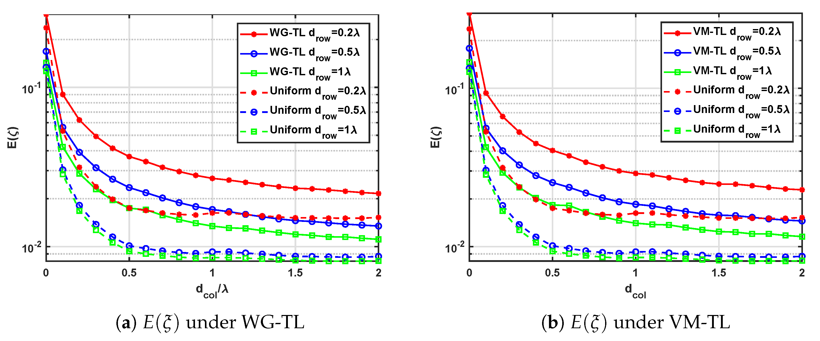
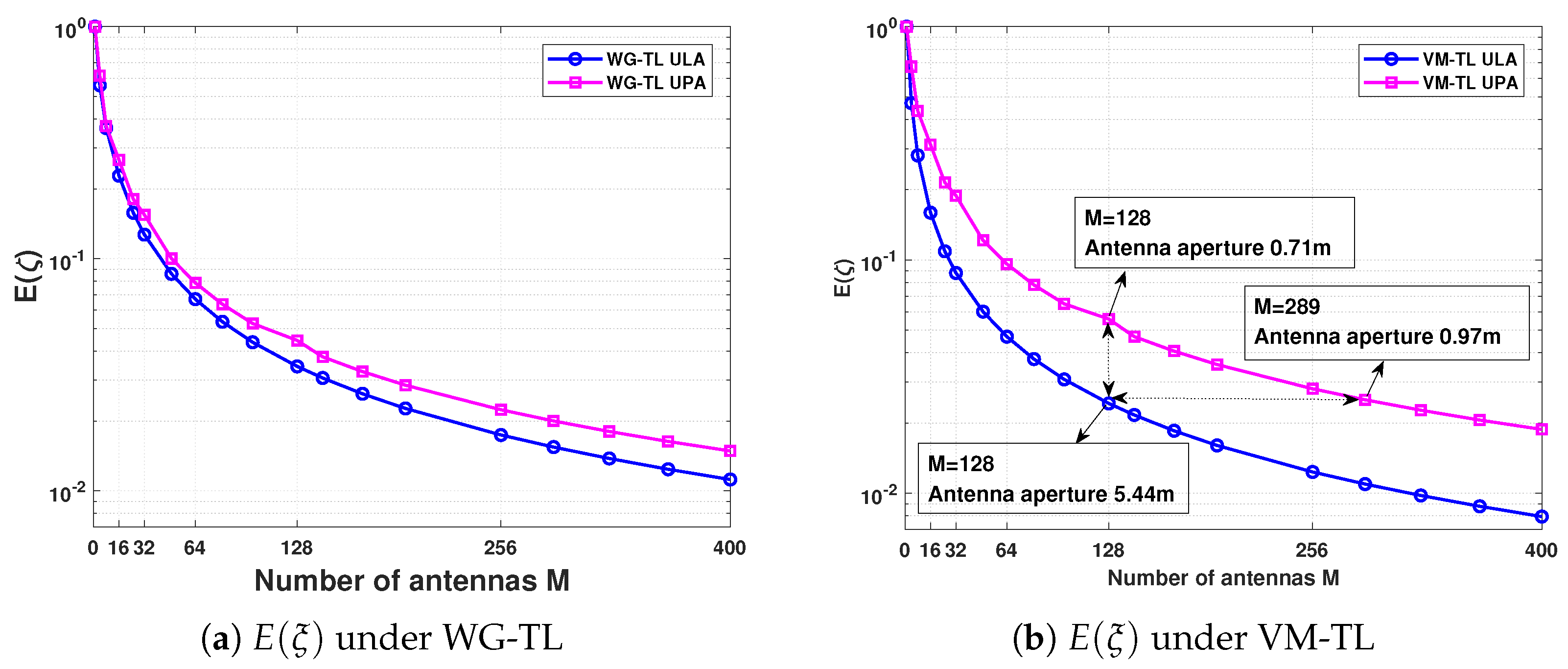
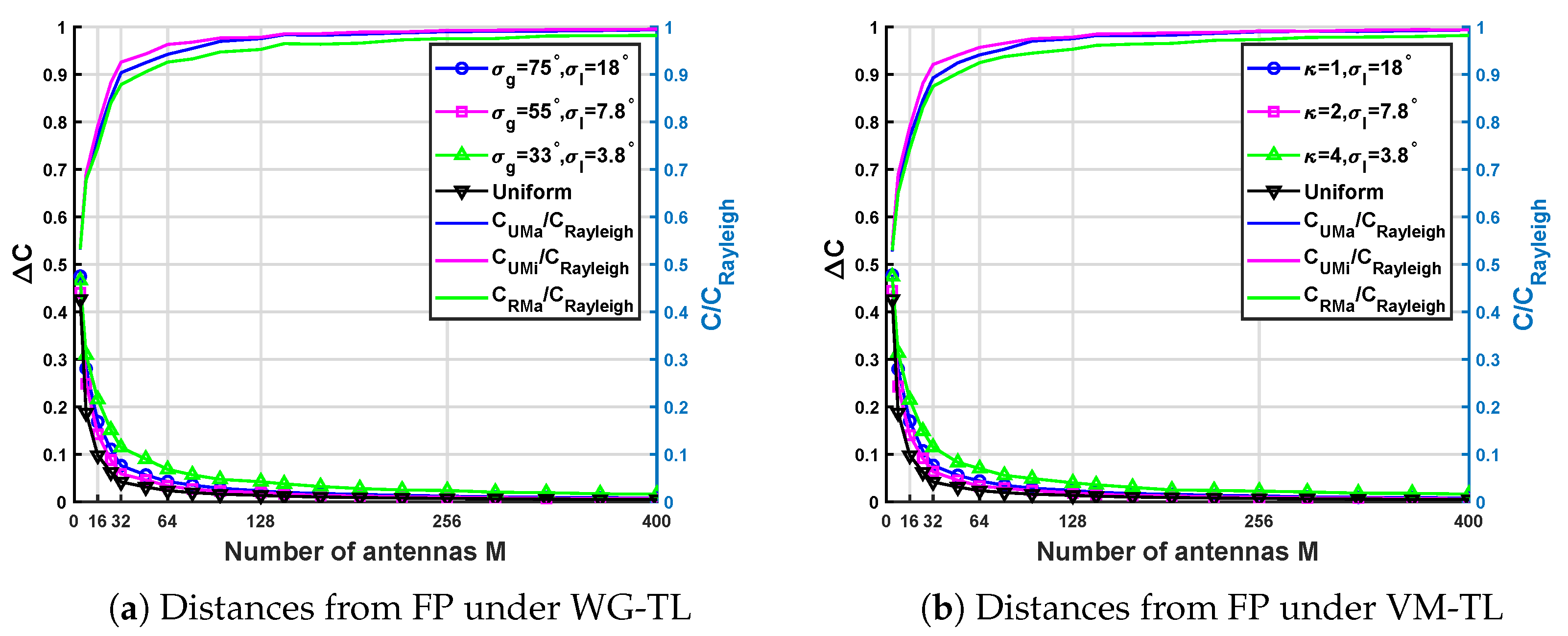
• We analyze the FP condition under different antenna spacing in the numerical simulations. It is noted that small antenna spacing, i.e., smaller than half-wavelength, leads to large inter-user interference. The effect of the antenna array on the FP condition is studied, and suitable spacing and array types are recommended.
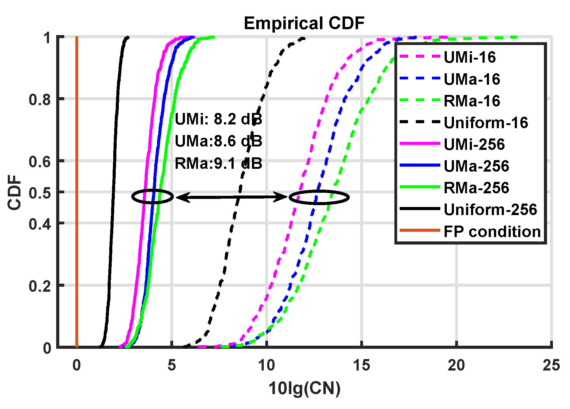
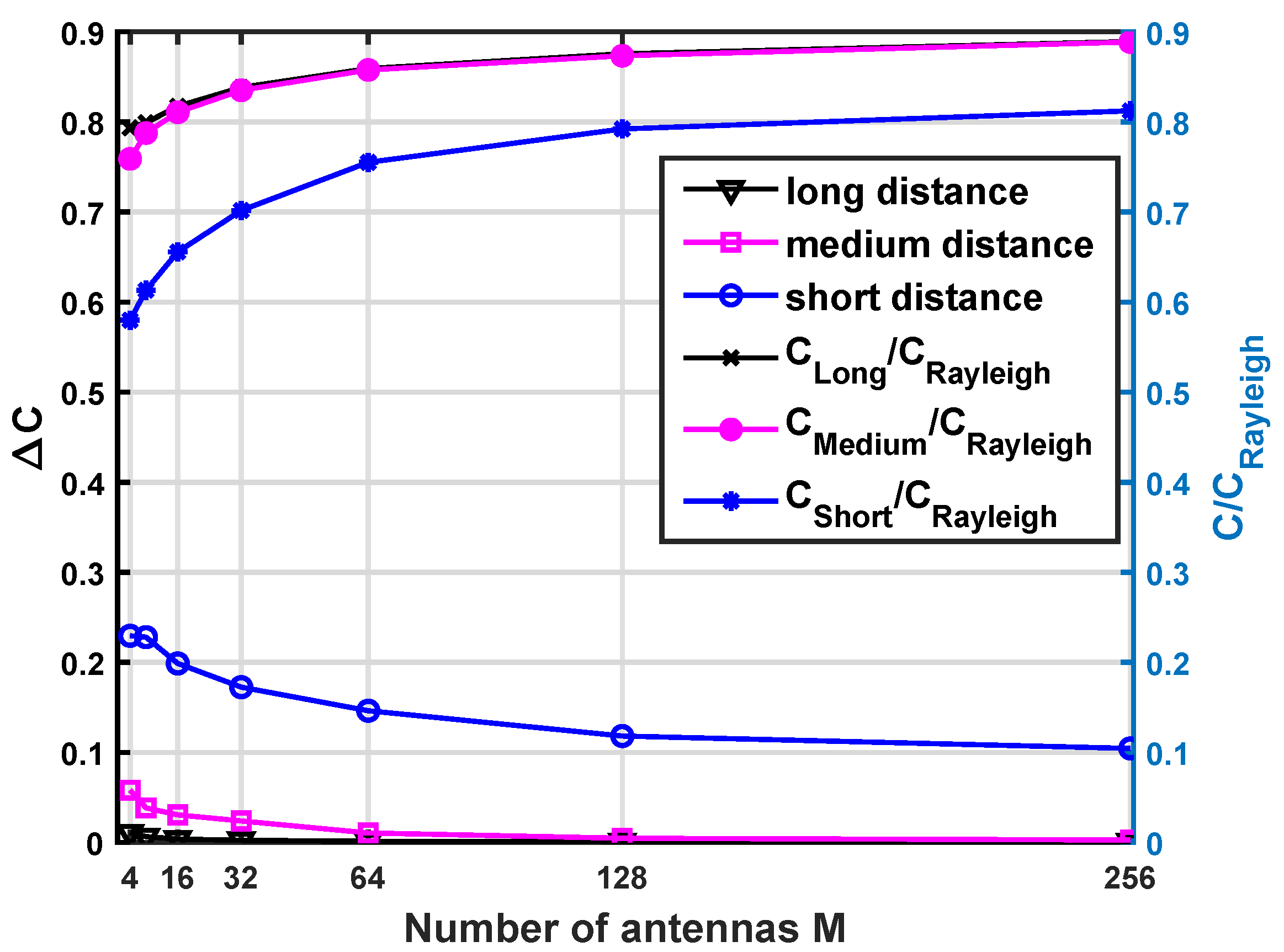
• The FP condition is also validated by practical measurements. It is observed that environments with larger angle spreads are more likely to satisfy the asymptotically FP condition. Moreover, users in significantly different propagation environments are more likely to have orthogonal channel vectors.

The remainder of the paper is outlined as follows. Section 2 briefly introduces the FP’s definition and the 3D MIMO channel model we adopt. In Section 3, the expectations and variances of the steering vector inner product are derived. Moreover, we theoretically analyze the asymptotically FP condition under WG-TL and VM-TL. Section 4 and Section 5 give FP’s numerical and measurement results under different scattering scenarios and antenna configurations. Finally, we conclude this paper in Section 6.

Notation: ${(·)}^T$ and ${(·)}^H$ denote the transpose and Hermitian transpose operation, respectively. ${\mathbb{C}}^{m\times n}$ represents a $m\times n$ dimensional matrix. The expectation and variance are denoted as $E(·)$ and $Var(·)$. The distributions of Von Mises, truncated Laplacian, wrapped Gaussian, complex Gaussian and uniform distributions are expressed as $\mathcal{V}\mathcal{M}(\mu ,k)$, $\mathcal{T}\mathcal{L}(\mu ,{\sigma }^2)$, $\mathcal{W}\mathcal{G}(\mu ,{\sigma }^2)$, $\mathcal{C}\mathcal{N}\left(\mu ,{\sigma }^2\right)$ and $\mathcal{U}(a,b)$, respectively. $J_n(·)$ and $I_n(·)$ are the nth order Bessel and modified Bessel function of the first kind, respectively.

2. Preliminaries

2.1. System Model

Consider an uplink single BS and multi-user massive MIMO system. K single-antenna users are simultaneously communicating with an M-antenna BS, where M is much larger than K. The system model can be given as [7]

$$\mathbf{y}=\sqrt{\rho }\mathbf{Gx}+\mathbf{n},$$

(1)

where $\mathbf{x}={[x_1,x_2,\dots x_K]}^T$ denotes a $K\times 1$ vector transmitted by K users and meets $E\left(\right|x_k{|}^2)=1$. $\mathbf{y}$ is an $M\times 1$ vector received by the BS. $\mathbf{G}=[{\mathbf{g}}_1,{\mathbf{g}}_2,\dots ,{\mathbf{g}}_K]$ is the channel matrix and ${\mathbf{g}}_k\in {\mathbb{C}}^{M\times 1}$ denotes the channel vector between the kth user and the BS. n is the additive noise vector and its components follow the zero-mean and unit-variance complex Gaussian distribution, i.e., $\mathcal{C}\mathcal{N}\left(0,1\right)$. $\rho$ represents the transmitted signal-to-noise ratio (SNR).

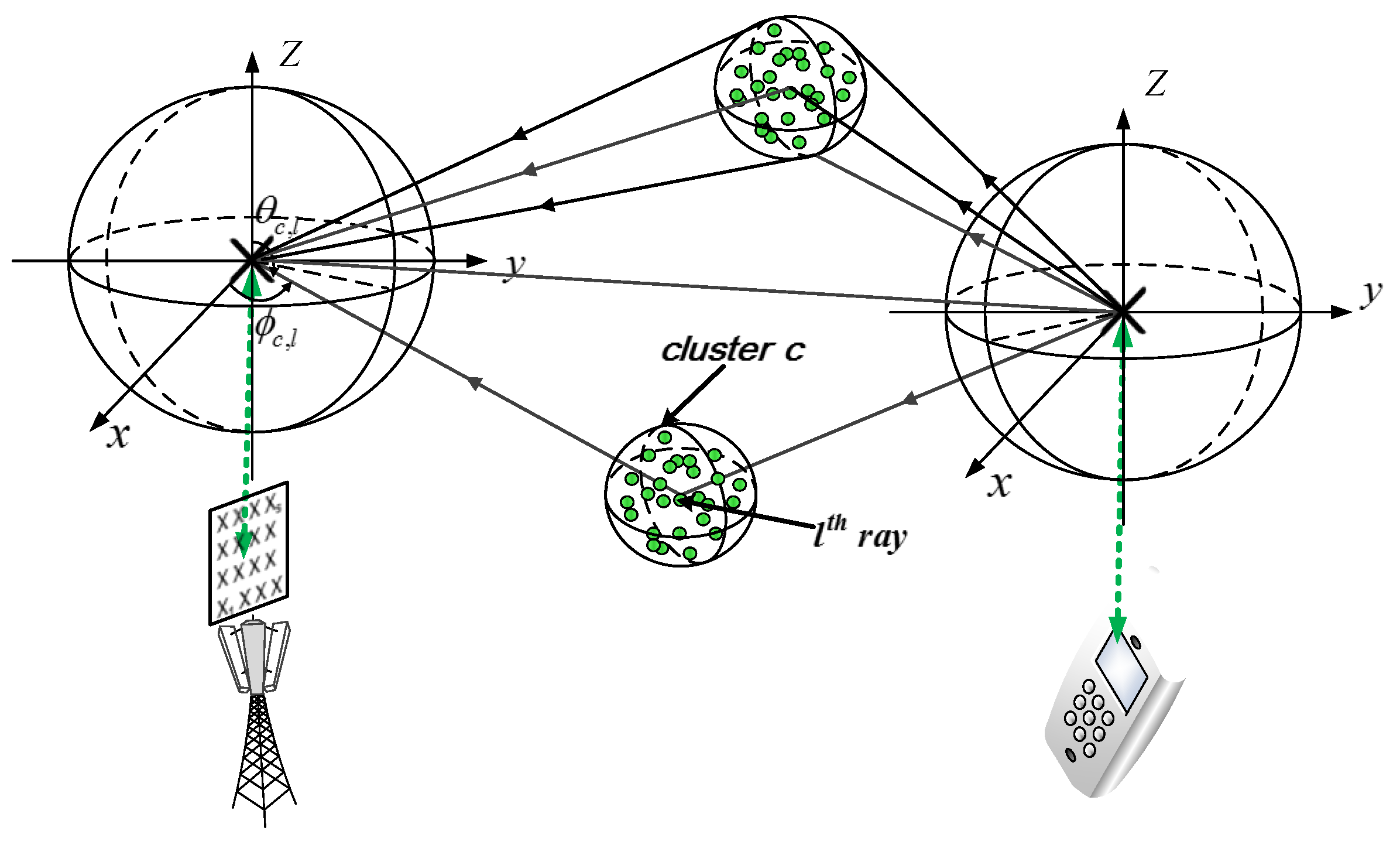
2.2. 3D MIMO Channel Model

In this paper, the 3D MIMO Geometry Based Stochastical channel model (GBSM) is adopted due to its wide application in both academics and standards [5,34]. In general, the wireless channel vector is a combination of the antenna response and the pure channel impulse response [34,35]. A cluster-based 3D MIMO channel model is illustrated in Figure 1, where each sphere represents a cluster and the dots inside it are similar rays of the cluster [5,36]. It can be seen the 3D MIMO channel is superimposed by the rays in each cluster. The wave line of each ray is represented by the azimuth AOA ${\varphi }_{c,l}$ and elevation AOA ${\theta }_{c,l}$ in a spherical coordinate together, and they can be fitted by some statistical distributions based on practical field channel measurements [34,35].

Figure 1. The illustration of a 3D MIMO channel model [5].

Assuming mutual coupling does not exist between isotropic antenna elements, the channel vector of the kth user can be simplistically expressed as

$$\begin{array}{cc}\hfill {\mathbf{g}}_k& =\sqrt{{\beta }_k}\sum _{c=1}^C\sqrt{\frac{p_{k,c}}{L}}\sum _{l=1}^L{\alpha }_{k,c,l}\mathbf{w}({\varphi }_{k,c,l},{\theta }_{k,c,l})\hfill \\ \hfill & \stackrel{\left(a\right)}{=}\sum _{s=1}^S{\alpha }_s\mathbf{w}({\varphi }_s,{\theta }_s),\hfill \end{array}$$

(2)

where

• ${\beta }_k$ is the large-scale fading.
• C and L are the number of clusters (spheres in Figure 1) and rays per cluster (dots in each sphere in Figure 1), respectively.
• $p_{k,c}$ is the normalized power of the kth user’s cluster c.
• ${\alpha }_{k,c,l},{\varphi }_{k,c,l},{\theta }_{k,c,l}$ are the normalized complex amplitude, azimuth AOA, elevation AOA of the lth ray in the cth cluster for the kth user, respectively.
• ${\alpha }_{k,c,l}\sim \mathcal{C}\mathcal{N}(0,1)$.
• $\mathbf{w}({\varphi }_{k,c,l},{\theta }_{k,c,l})$ is the antenna array steering vector. And the element of $\mathbf{w}({\varphi }_{k,c,l},{\theta }_{k,c,l})$ is $w({\varphi }_{k,c,l},{\theta }_{k,c,l})=e^{j\frac{2\pi }{\lambda }(sin{\theta }_{k,c,l}cos{\varphi }_{k,c,l}{x}_m+sin{\theta }_{k,c,l}sin{\varphi }_{k,c,l}{y}_m+cos{\theta }_{k,c,l}{z}_m)}$ when each antenna radiation pattern is assumed to be omnidirectional. ${[x_m,y_m,z_m]}^T$ is the mth antenna element’s location vector in a Cartesian coordinate system.

The equality (a) in the formula (2) holds when we use subscript s to represent subscript (k,c,l) equivalently for a simplified representation. The element of $\mathbf{w}({\varphi }_s,{\theta }_s)$ is $w_{ms}=w_{m,k,c,l}$, and ${\alpha }_s=\sqrt{\frac{{\beta }_k{p}_{k,c}}{L}}{\alpha }_{k,c,l}$.

2.3. Favorable Propagation and Channel Capacity

According to [18], the FP condition is defined as

$${\mathbf{g}}_i^H{\mathbf{g}}_j=\left\{\begin{array}{cc}0,& i\ne j,\\ {∥{\mathbf{g}}_i∥}_2^2,& i=j.\end{array}\right.$$

(3)

Equation (3) is an ideal assumption, which usually does not hold in most of realistic scenarios. However, when the antenna number at BS tends to infinity, different users’ channel vectors will become asymptotically orthogonal. This is the asymptotically favorable propagation condition [7] in (4). When $i\ne j$, there is

$$\frac{1}{M}{\mathbf{g}}_i^H{\mathbf{g}}_j\to 0,M\to \infty .$$

(4)

Assuming the channel state information (CSI) is known to the BS [7] and considering the system model in (1), we express the massive MIMO system capacity as (5).

$$\begin{array}{cc}\hfill C& ={log}_{2}det({\mathbf{I}}_K+\rho {\mathbf{G}}^H\mathbf{G})\hfill \\ \hfill & \stackrel{\left(b\right)}{=}\mathrm{lo}{\mathrm{g}}_2\det ({\mathbf{I}}_K+\rho diag({∥{\mathbf{g}}_1∥}_2^2,{∥{\mathbf{g}}_2∥}_2^2,\dots ,{∥{\mathbf{g}}_K∥}_2^2))\hfill \\ \hfill & =\sum _{k=1}^K{log}_2(1+\rho {∥{\mathbf{g}}_k∥}_2^2),\hfill \end{array}$$

(5)

where $diag(a_1,a_2,\dots ,a_n)$ represents a diagonal matrix and $a_n$ is the diagonal element. The equality (b) in the formula (5) holds only if the FP condition is satisfied. The expression (5) shows that different users’ channel vectors are mutually independent and inter-user interference does not exist. Besides, it shows that the channel under FP provides the maximum capacity [6].

3. Asymptotically Favorable Propagation Analysis Using WG-TL and VM-TL

3.1. Asymptotically FP Analysis

The asymptotically FP can be expressed as (6) based on the channel model in (2).

$$\begin{array}{cc}\hfill \frac{1}{M}{\mathbf{g}}_i^H{\mathbf{g}}_j& =\frac{1}{M}\sum _{s=1}^S{\alpha }_s^{*}{\mathbf{w}}^H({\varphi }_s,{\theta }_s)\sum _{p=1}^P{\alpha }_p\mathbf{w}({\varphi }_p,{\theta }_p)\hfill \\ \hfill & =\sum _{s=1}^S\sum _{p=1}^P{\alpha }_s^{*}{\alpha }_p·\frac{1}{M}\sum _{m=1}^M{w}_{ms}^{*}{w}_{mp}.\hfill \end{array}$$

(6)

Since the term ${\alpha }_s^{*}{\alpha }_p$ is limited by the large-scale fading parameter $\sqrt{{\beta }_i{\beta }_j}$, the condition

$$\begin{array}{cc}\hfill \xi & =\frac{1}{M}{\mathbf{w}}^H({\varphi }_s,{\theta }_s)\mathbf{w}({\varphi }_p,{\theta }_p)\hfill \\ \hfill & =\frac{1}{M}\sum _{m=1}^M{w}_{ms}^{*}{w}_{mp}\to 0,M\to \infty ,\hfill \end{array}$$

(7)

is sufficient to satisfy the asymptotically FP condition in (4).

In practical massive MIMO systems, $\xi$ in (7) can be calculated as

$$\begin{array}{cc}\hfill \xi & =\frac{1}{M}\sum _{m=1}^M\left(e^{j\frac{2\pi }{\lambda }(sin{\theta }_{s}cos{\varphi }_s{x}_m+sin{\theta }_{s}sin{\varphi }_s{y}_m+cos{\theta }_s{z}_m)}\right.\hfill \\ \hfill & \left.\times e^{-j\frac{2\pi }{\lambda }(sin{\theta }_{p}cos{\varphi }_p{x}_m+sin{\theta }_{p}sin{\varphi }_p{y}_m+cos{\theta }_p{z}_m)}\right),\hfill \end{array}$$

(8)

Equation (8) is a general formula for arbitrary types of antenna arrays with only different location vectors being generated [21,37].

3.2. Statistical Property Analysis under Generalized Angle Distributions

To derive the formula (7) holds is to prove the expectation $E\left(\xi \right)$ and variance $Var\left(\xi \right)$ both equal to zero based on the statistical theory [38]. Considering the rays between different users and the BS follow i.i.d. distribution, $E\left(\xi \right)$ and $Var\left(\xi \right)$ are converted to (9) and (10). Therefore, we need to derive $E\left(w_{ms}^{*}\right)$, $E\left(w_{ms}\right)$, and $E\left(w_{ms}^{*}{w}_{m^{\prime }s}\right)$ in (9) and (10) to get $E\left(\xi \right)$ and $Var\left(\xi \right)$, where $E_{{\varphi }_0}(·)$ is the expectation operator for mean azimuth AOAs of different users.

$$\begin{array}{cc}\hfill E\left(\xi \right)& =\frac{1}{M}\sum _{m=1}^{M}E\left(w_{ms}^{*}{w}_{mp}\right)=\frac{1}{M}\sum _{m=1}^{M}E\left(w_{ms}^{*}\right)E\left(w_{mp}\right)\hfill \\ \hfill & =\frac{1}{M}\sum _{m=1}^M{E}_{{\varphi }_0}\left\{E_{AOA}\left(w_{ms}^{*}\right)\right\}{E}_{{\varphi }_0}\left\{E_{AOA}\left(w_{mp}\right)\right\}.\hfill \end{array}$$

(9)

$$\begin{array}{cc}\hfill Var\left(\xi \right)& =E\left(\xi {\xi }^{*}\right)-E\left(\xi \right)E\left({\xi }^{*}\right)\hfill \\ \hfill & =\frac{1}{M^2}\sum _{m=1}^M\sum _{m^{\prime }=1}^M\left\{E\left(w_{ms}^{*}{w}_{m^{\prime }s}{w}_{m^{\prime }p}^{*}{w}_{mp}\right)\right.-\left.E\left(w_{ms}^{*}{w}_{mp}\right)E\left(w_{m^{\prime }s}{w}_{m^{\prime }p}^{*}\right)\right\}\hfill \\ \hfill & =\frac{1}{M^2}\sum _{m=1}^M\sum _{m^{\prime }=1}^M\left\{E_{{\varphi }_0}\left\{E_{AOA}\left(w_{ms}^{*}{w}_{m^{\prime }s}\right)\right\}{E}_{{\varphi }_0}\left\{E_{AOA}\left(w_{m^{\prime }p}^{*}{w}_{mp}\right)\right\}\right.\hfill \\ \hfill & -\left.E_{{\varphi }_0}\left\{E_{AOA}\left(w_{ms}^{*}\right)\right\}{E}_{{\varphi }_0}\left\{E_{AOA}\left(w_{mp}\right)\right\}\left\{E_{AOA}\left(w_{m^{\prime }s}\right)\right\}{E}_{{\varphi }_0}\left\{E_{AOA}\left(w_{m^{\prime }p}^{*}\right)\right\}\right\}.\hfill \end{array}$$

(10)

Referring to some measurement results [10] and the standard 3D MIMO channel model [34,35], VM or WG is used to model the azimuth angle distribution and TL is used to model the elevation angle distribution. The probability density functions (PDFs) of VM, WG, TL distributions are given in Table 1. The corresponding curves are plotted in Figure 2. Different PDFs characterize different spatial angular dispersions which directly affect the spatial correlation. It can be seen that the shape of the TL distribution is the narrowest, which means most angles are concentrated around the mean value. And this characteristic fits well with the elevation angle due to the sparse scatterers in the vertical dimension. Besides, the WG distribution’s curve is very similar to that of the VM distribution’s, especially for smaller angle spreads. As an ideal case, the uniform distribution which represents rich scattering environments, is also given in Table 1 and Figure 2. The uniform distribution $\mathcal{U}(-\pi ,\pi )$ has the largest angle spread of $104^{\circ }$ for azimuth angles.

Table 1. PDFs of different angle distributions.

Distribution	PDF	Domain
Wrapped Gaussian [34]	$\frac{Q_g}{\sqrt{2\pi }{\sigma }_g}{e}^{\frac{-{(\varphi -{\varphi }_0)}^2}{2{\sigma }_g^2}}$	$-\pi \le \varphi -{\varphi }_0\le \pi$
Von Mises [31]	$\frac{e^{\kappa cos(\varphi -{\varphi }_0)}}{2\pi I_0\left(\kappa \right)}$	$-\pi \le \varphi -{\varphi }_0\le \pi$
Truncated Laplacian [34]	$\frac{Q_l}{\sqrt{2}{\sigma }_l}{e}^{-\frac{\sqrt{2}\left|\theta -{\theta }_0\right|}{{\sigma }_l}}$	$-\frac{\pi }{2}\le \theta -{\theta }_0\le \frac{\pi }{2}$
Uniform [21]	$\frac{1}{2\pi }$	$-\pi \le \varphi -{\varphi }_0\le \frac{\pi }{2}$
	$\frac{1}{\pi }$	$-\frac{\pi }{2}\le \theta -{\theta }_0\le \pi$

Notes: ϕ₀, θ₀, σ_g, σ₁ are the mean azimuth AOA, mean elevation AOA, azimuth AOA spread, and elevation AOA spread, respectively. k is the concentration factor. Q_g and Q_l are the normalization factors, which make the integral of PDFs on the domain equal to 1.

Figure 2. PDFs of different angle distributions.

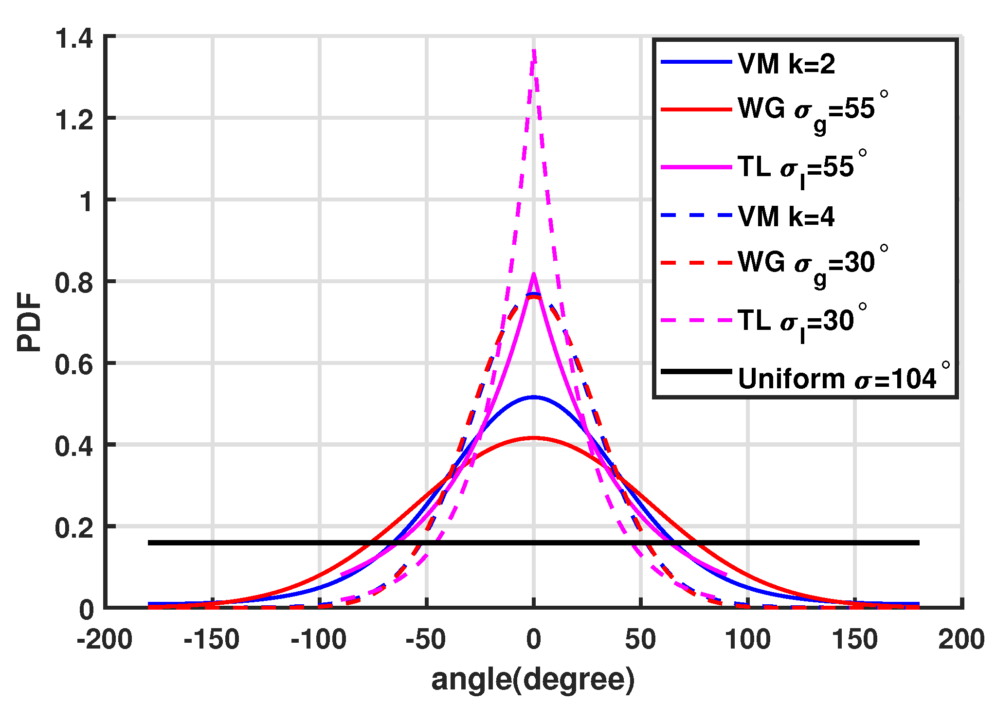
3.2.1. Von Mises and Truncated Laplacian Distributions

Assume azimuth AOAs $\varphi$ follow $\mathcal{V}\mathcal{M}({\varphi }_0^i,\kappa )$ and elevation AOAs $\theta$ follow $\mathcal{T}\mathcal{L}({\theta }_0^i,{\sigma }_l)$, where ${\varphi }_0^i$ and ${\theta }_0^i$ are the mean azimuth AOA and mean elevation AOA of the ith user, respectively. Assume that users are uniformly distributed around the BS, i.e., ${\varphi }_0^i$ follows $\mathcal{U}(-\pi ,\pi )$. We are now deriving the expectation $E_{vl}\left(\xi \right)$ and variance $Va{r}_{vl}\left(\xi \right)$ in (9) and (10).

$$\begin{array}{cc}\hfill & E_{AOA}\left(w_{ms}^{*}\right)=\underset{-\frac{\pi }{2}}{\overset{\frac{\pi }{2}}{\int }}\underset{-\pi }{\overset{\pi }{\int }}{e}^{j\frac{2\pi }{\lambda }(sin\theta cos\varphi x_m+sin\theta sin\varphi y_m+cos\theta z_m)}\frac{e^{\kappa cos(\Delta \varphi )}}{2\pi I_0\left(\kappa \right)}\frac{Q_l}{\sqrt{2}{\sigma }_l}{e}^{-\frac{\sqrt{2}\left|\Delta \theta \right|}{{\sigma }_l}}d\Delta \varphi d\Delta \theta .\hfill \end{array}$$

(11)

Firstly, $E_{AOA}\left(w_{m^{\prime }p}^{*}\right)$ in (9) and (10) can be expressed as (11), where $\mathrm{\Delta }\varphi = \varphi -{\varphi }_0$ and $\mathrm{\Delta }\theta = \theta -{\theta }_0$ in Table 1. Then we utilize the product-to-sum transform, Bessel expansion in (12), and Euler transform $cos\left(n\mathrm{\Delta }\varphi \right)=\frac{e^{jn\mathrm{\Delta }\varphi }+e^{-jn\mathrm{\Delta }\varphi }}{2}$ and compute the integral according to the integral representation of Bessel function in (13).

$$e^{\kappa cos\left(\mathrm{\Delta }\varphi \right)}=I_0\left(\kappa \right)+2\sum _{n=1}^{\infty }{I}_n\left(\kappa \right)cos\left(n\mathrm{\Delta }\varphi \right).$$

(12)

$$\begin{array}{c}\hfill J_n\left(v\right)=\frac{1}{2\pi }\underset{-\pi }{\overset{\pi }{\int }}{e}^{j(n\theta -vsin\theta )}d\theta .\end{array}$$

(13)

Furtherly, using the similar process with Equation (18) to (29) in [17], (11) is finally given as (14),

$$\begin{array}{c}\hfill E_{AOA}\left(w_{ms}^{*}\right)=C_{vl}\left({\chi }_0{\mathrm{\Gamma }}_0(-x_m,-y_m,z_m)+2\sum _{n=1}^{\infty }{\chi }_{n}cos(n({\varphi }_0^i-{\Omega }_m){\mathrm{\Gamma }}_n(-x_m,-y_m,z_m)\right),\end{array}$$

(14)

where

• $C_{vl}$ is the constant component associated with the distribution of AOA,

  $$C_{vl}=\frac{Q_l}{\sqrt{2}{\sigma }_l{I}_0\left(\kappa \right)}.$$

  (15)
• $\{{\chi }_n,n=0,1,2,\dots \}$ are given by

  $${\chi }_n={\left(-\mathrm{j}\right)}^n{I}_n\left(\kappa \right).$$

  (16)
• $\{{\mathrm{\Gamma }}_n(x,y,z),n=0,1,2,\dots \}$ are the functions of antenna coordinates in (17). ${\mathrm{\Omega }}_m$ is equal to $arctan\left(\frac{y_m}{x_m}\right)$. $\{a_l,l=0,1,2,\dots \}$ are the Fourier series coefficients of $e^{-\frac{\sqrt{2}\left|\theta -\frac{\pi }{2}\right|}{{\sigma }_l}}$.

Finally, (18) and (19) are derived. The detailed proof is given in Appendix A.

$$\begin{array}{cc}\hfill {\mathrm{\Gamma }}_n(x,y,z)& =\sum _{l=0}^{\infty }{a}_l\sum _{\beta =-\infty }^{\infty }{\left(j\right)}^{\beta }{J}_{\beta }\left(\frac{2\pi }{\lambda }{z}_m\right)\frac{\pi }{2}\{cos\left(\frac{l\pi }{2}\right)[cos\left(\frac{l+\beta }{2}\pi \right)J_{\frac{n-l-\beta }{2}}(\frac{\pi }{\lambda }sec{\mathrm{\Omega }}_m{x}_m)J_{\frac{n+l+\beta }{2}}(\frac{\pi }{\lambda }sec{\mathrm{\Omega }}_m{x}_m)\hfill \\ \hfill & +cos\left(\frac{l-\beta }{2}\pi \right)J_{\frac{n-l+\beta }{2}}(\frac{\pi }{\lambda }sec{\mathrm{\Omega }}_m{x}_m)J_{\frac{n+l-\beta }{2}}(\frac{\pi }{\lambda }sec{\mathrm{\Omega }}_m{x}_m)]+sin\left(\frac{l\pi }{2}\right)[sin\left(\frac{l+\beta }{2}\pi \right)J_{\frac{n-l-\beta }{2}}(\frac{\pi }{\lambda }sec{\mathrm{\Omega }}_m{x}_m)\hfill \\ \hfill & \times J_{\frac{n+l+\beta }{2}}(\frac{\pi }{\lambda }sec{\mathrm{\Omega }}_m{x}_m)+sin\left(\frac{l-\beta }{2}\pi \right)J_{\frac{n-l+\beta }{2}}(\frac{\pi }{\lambda }sec{\mathrm{\Omega }}_m{x}_m)J_{\frac{n+l-\beta }{2}}(\frac{\pi }{\lambda }sec{\mathrm{\Omega }}_m{x}_m)\left]\right\}.\hfill \end{array}$$

(17)

$$\begin{array}{c}\hfill E_{vl}\left(\xi \right)=\frac{{C_{vl}}^2}{M}\sum _{m=1}^M{{\chi }_0}^2{\mathrm{\Gamma }}_0(x_m,y_m,-z_m){\mathrm{\Gamma }}_0(-x_m,-y_m,z_m).\end{array}$$

(18)

$$\begin{array}{cc}\hfill Va{r}_{vl}\left(\xi \right)& =\frac{1}{M^2}\sum _{m=1}^M\sum _{m^{\prime }=1}^M{C_{vl}}^2{{\chi }_0}^2{\mathrm{\Gamma }}_0(x_m-x_{m^{\prime }},y_m-y_{m^{\prime }},z_{m^{\prime }}-z_m){\mathrm{\Gamma }}_0(x_{m^{\prime }}-x_m,y_{m^{\prime }}-y_m,z_m-z_{m^{\prime }})\hfill \\ \hfill & -{C_{vl}}^4{{\chi }_0}^4{\mathrm{\Gamma }}_0(x_m,y_m,-z_m){\mathrm{\Gamma }}_0(-x_m,-y_m,z_m){\mathrm{\Gamma }}_0(x_{m^{\prime }},y_{m^{\prime }},-z_{m^{\prime }}){\mathrm{\Gamma }}_0(-x_{m^{\prime }},-y_{m^{\prime }},z_{m^{\prime }}).\hfill \end{array}$$

(19)

$$\begin{array}{cc}\hfill {\mathrm{\Gamma }}_0(x,y,z)& \approx \sum _{l=0}^L{a}_l\sum _{\beta =-B}^B{\left(j\right)}^{\beta }{J}_{\beta }\left(\frac{2\pi }{\lambda }{z}_m\right)\frac{\pi }{2}\{cos\left(\frac{l\pi }{2}\right)[cos\left(\frac{l+\beta }{2}\pi \right)J_{\frac{-l-\beta }{2}}(\frac{\pi }{\lambda }sec{\mathrm{\Omega }}_m{x}_m)J_{\frac{l+\beta }{2}}(\frac{\pi }{\lambda }sec{\mathrm{\Omega }}_m{x}_m)\hfill \\ \hfill & +cos\left(\frac{l-\beta }{2}\pi \right)J_{\frac{\beta -l}{2}}(\frac{\pi }{\lambda }sec{\mathrm{\Omega }}_m{x}_m)J_{\frac{l-\beta }{2}}(\frac{\pi }{\lambda }sec{\mathrm{\Omega }}_m{x}_m)]+sin\left(\frac{l\pi }{2}\right)[sin\left(\frac{l+\beta }{2}\pi \right)J_{\frac{-l-\beta }{2}}(\frac{\pi }{\lambda }sec{\mathrm{\Omega }}_m{x}_m)\hfill \\ \hfill & \times J_{\frac{l+\beta }{2}}(\frac{\pi }{\lambda }sec{\mathrm{\Omega }}_m{x}_m)+sin\left(\frac{l-\beta }{2}\pi \right)J_{\frac{\beta -l}{2}}(\frac{\pi }{\lambda }sec{\mathrm{\Omega }}_m{x}_m)J_{\frac{l-\beta }{2}}(\frac{\pi }{\lambda }sec{\mathrm{\Omega }}_m{x}_m)\left]\right\}.\hfill \end{array}$$

(20)

As observed in (18), the convergence property of $E_{vl}\left(\xi \right)$ is determined by ${\mathrm{\Gamma }}_0$ function due to the constant values of ${C_{gl}}^2$ and ${{{\rm Y}}_0}^2$. Hence, the convergence property of ${\mathrm{\Gamma }}_0$ function is discussed. The coefficient $a_l$ tends to zero with l increasing based on the property of Fourier series coefficients. And $|J_{\left|\beta \right|}\left|\right(\left|x\right|)$ is limited by 1 for any integer $\beta$ and $J_v\left(x\right)J_{-v}\left(x\right)$ is a finite value based on the properties of Bessel function [39], (9.1.5, 9.1.60 and 9.1.14). Besides, as $\left|x\right|$ or $\left|\beta \right|$ increases, $|J_{\left|\beta \right|}\left|\right(\left|x\right|)$ decays to zero. Furthermore, the functions of sinusoidal, cosine and arc-cosine are all smaller than one. Therefore, it can be seen in (20) that ${\mathrm{\Gamma }}_0$ function is summed by a number of finite values. When the antenna number increases to infinity, i.e., $M\to \infty$, ${\mathrm{\Gamma }}_0$ function tends to zero and $E_{vl}\left(\xi \right)\to 0$.

Similar with the above analysis, it can be inferred that the convergence property of $Va{r}_{vl}\left(\xi \right)$ in (19) is also determined by ${\mathrm{\Gamma }}_0$ function. As the antenna number M increases to infinity, ${\mathrm{\Gamma }}_0$ function tends to zero and the variance $Va{r}_{vl}\left(\xi \right)$ converges to zero, i.e., $Va{r}_{vl}\left(\xi \right)\to 0$. It is concluded that the asymptotically FP condition is satisfied under the VM-TL distribution based on the analysis of the convergence properties of $E_{vl}\left(\xi \right)$ and $Va{r}_{vl}\left(\xi \right)$.

3.2.2. Wrapped Gaussian and Truncated Laplacian Distributions

Assuming azimuth AOAs $\varphi$ follow $\mathcal{W}\mathcal{G}({\varphi }_0^i,{\sigma }_g)$ and elevation AOAs $\theta$ follow $\mathcal{T}\mathcal{L}({\theta }_0^i,{\sigma }_l)$, (9) and (10) are expressed as (21) and (22),

$$\begin{array}{c}\hfill E_{gl}\left(\xi \right)=\frac{{C_{gl}}^2}{M}\sum _{m=1}^M{{{\rm Y}}_0}^2{\mathrm{\Gamma }}_0(x_m,y_m,z_m){\mathrm{\Gamma }}_0(-x_m,-y_m,-z_m),\end{array}$$

(21)

$$\begin{array}{cc}\hfill Va{r}_{gl}\left(\xi \right)& =\frac{1}{M^2}\sum _{m=1}^M\sum _{m^{\prime }=1}^M{C_{gl}}^2{{{\rm Y}}_0}^2{\mathrm{\Gamma }}_0(x_m-x_{m^{\prime }},y_m-y_{m^{\prime }},z_m-z_{m^{\prime }}){\mathrm{\Gamma }}_0(x_{m^{\prime }}-x_m,y_{m^{\prime }}-y_m,z_{m^{\prime }}-z_m)\hfill \\ \hfill & -{C_{gl}}^4{{{\rm Y}}_0}^4{\mathrm{\Gamma }}_0(x_m,y_m,z_m){\mathrm{\Gamma }}_0(-x_m,-y_m,-z_m){\mathrm{\Gamma }}_0(x_{m^{\prime }},y_{m^{\prime }},z_{m^{\prime }}){\mathrm{\Gamma }}_0(-x_{m^{\prime }},-y_{m^{\prime }},-z_{m^{\prime }}),\hfill \end{array}$$

(22)

where

• $C_{gl}=\frac{Q_g{Q}_l}{\sqrt{2}{\sigma }_l}$ is the constant component associated with the AOAs’ distribution, and $Q_g=\frac{1}{erf\left(\frac{\pi }{\sqrt{2}{\sigma }_g}\right)}$, $Q_l=\frac{1}{1-e^{\frac{-\sqrt{2}\pi }{2{\sigma }_l}}}$.
• $\{{{\rm Y}}_n,n=0,1,2,\dots \}$ are given by

  $$\begin{array}{cc}\hfill {{\rm Y}}_n& =\frac{1}{2}{\left(j\right)}^n{e}^{-\frac{{\left(n{\sigma }_g\right)}^2}{2}}[erf(\frac{\pi }{\sqrt{2}{\sigma }_g}-j\frac{n{\sigma }_g}{\sqrt{2}})\hfill \\ \hfill & +erf(\frac{\pi }{\sqrt{2}{\sigma }_g}+j\frac{n{\sigma }_g}{\sqrt{2}})],\hfill \end{array}$$

  (23)

  and $erf(a+jb)$ is the error function for complex argument [39].
• $\{{\mathrm{\Gamma }}_n(x,y,z),n=0,1,2,\dots \}$ and ${\mathrm{\Omega }}_m$ are same with them in (11), (14) and (17).

The detailed proof is similar to the VM-TL distribution, which is given in our previous work in [17]. When the antenna number m tends to infinity, the analysis of the convergence properties of $E_{gl}\left(\xi \right)$ and ${Var}_{gl}\left(\xi \right)$ is similar with that of $E_{vl}\left(\xi \right)$ and ${Var}_{vl}\left(\xi \right)$, and we omit the derivation process.

3.2.3. Uniform Distributions

Assuming azimuth AOAs $\varphi$ follow $\mathcal{U}(-\pi ,\pi )$ and elevation AOAs $\theta$ follow $\mathcal{U}(-\frac{\pi }{2},\frac{\pi }{2})$, (9) and (10) are expressed similarly with (18), (19), (21) and (22). This result is proved in (24)–(26) when we make $\kappa$ in VM tend to zero, ${\sigma }_g$ in WG and ${\sigma }_l$ in TL tend to infinity.

• When we make $\kappa$ in VM be zero, we have

  $$\begin{array}{c}\hfill \frac{e^{\kappa cos(\varphi -{\varphi }_0)}}{2\pi I_0\left(\kappa \right)}\stackrel{\kappa =0}{=}\frac{e^{0cos(\varphi -{\varphi }_0)}}{2\pi I_0\left(0\right)}=\frac{1}{2\pi }.\end{array}$$

  (24)
• When we make ${\sigma }_g$ in WG and ${\sigma }_l$ in TL tend to infinity and utilize the L${}^{\prime }$ Hospital (LH) rule, we have

  $$\begin{array}{c}\hfill \underset{{\sigma }_g\to \infty }{lim}\frac{Q_g}{\sqrt{2\pi }{\sigma }_g}{e}^{\frac{-{(\varphi -{\varphi }_0)}^2}{2{\sigma }_g^2}}=\underset{{\sigma }_g\to \infty }{lim}\frac{\frac{1}{\sqrt{2\pi }{\sigma }_g}}{erf\left(\frac{\pi }{\sqrt{2}{\sigma }_g}\right)}\stackrel{LH}{=}\frac{1}{2\pi },\end{array}$$

  (25)

  $$\begin{array}{c}\hfill \underset{{\sigma }_l\to \infty }{lim}\frac{Q_l}{\sqrt{2}{\sigma }_l}{e}^{-\frac{\sqrt{2}\left|\theta -{\theta }_0\right|}{{\sigma }_l}}=\underset{{\sigma }_l\to \infty }{lim}\frac{\frac{1}{\sqrt{2}{\sigma }_l}}{1-e^{-\frac{\sqrt{2}\pi }{2{\sigma }_l}}}\stackrel{LH}{=}\frac{1}{\pi }.\end{array}$$

  (26)

In this case, WG, VM, and TL distributions converge to uniform distributions. Therefore, WG, VM, and TL are the generalized expansions of uniform distributions, which are more practical for the FP condition in the real scenario.

3.2.4. Azimuth Angle Distributions

Assuming the antenna elements are only deployed in the azimuth domain, i.e., ULA in [16,18,21], rays can be distinguished only in the azimuth domain. We can set $\theta =\frac{\pi }{2}$, i.e., $\theta -{\theta }_0=0$ in TL in Table 1, which indicates that the azimuth angle distribution is only a particular case of our derivation.

4. Numerical Simulations

In order to analyze the FP condition under generalized angle distributions, we simulate the performance utilizing the IMT-2020 5G channel simulation platform. This platform is developed based on the 5G channel model standards 3GPP TR 38.901 [34] and ITU-R M.2412 [35]. Three typical scenarios, i.e., UMa, UMi, and RMa, are selected, and different types of antenna arrays are configured. Table 2 shows the detailed simulation parameters (http://www.zjhlab.net/publications/imt-2020cmbupt/) (accessed on 30 May 2022).

Table 2. Simulation parameters [34,35].

Scenarios (NLOS)	UMa	UMi	RMa
Center frequency		3.5 GHz
Number of clusters	20	19	10
Number of rays per cluster	20	20	20
Concentration factor $\kappa$	1	2	4
Inter-cluster azimuth angle spread ${\sigma }_g$	75${}^{\circ }$	55${}^{\circ }$	33${}^{\circ }$
Inter-cluster elevation angle spread ${\sigma }_l$	18${}^{\circ }$	7.8${}^{\circ }$	3.8${}^{\circ }$
Intra-cluster azimuth angle spread	15${}^{\circ }$	22${}^{\circ }$	3${}^{\circ }$
Intra-cluster elevation angle spread	7${}^{\circ }$	7${}^{\circ }$	3${}^{\circ }$

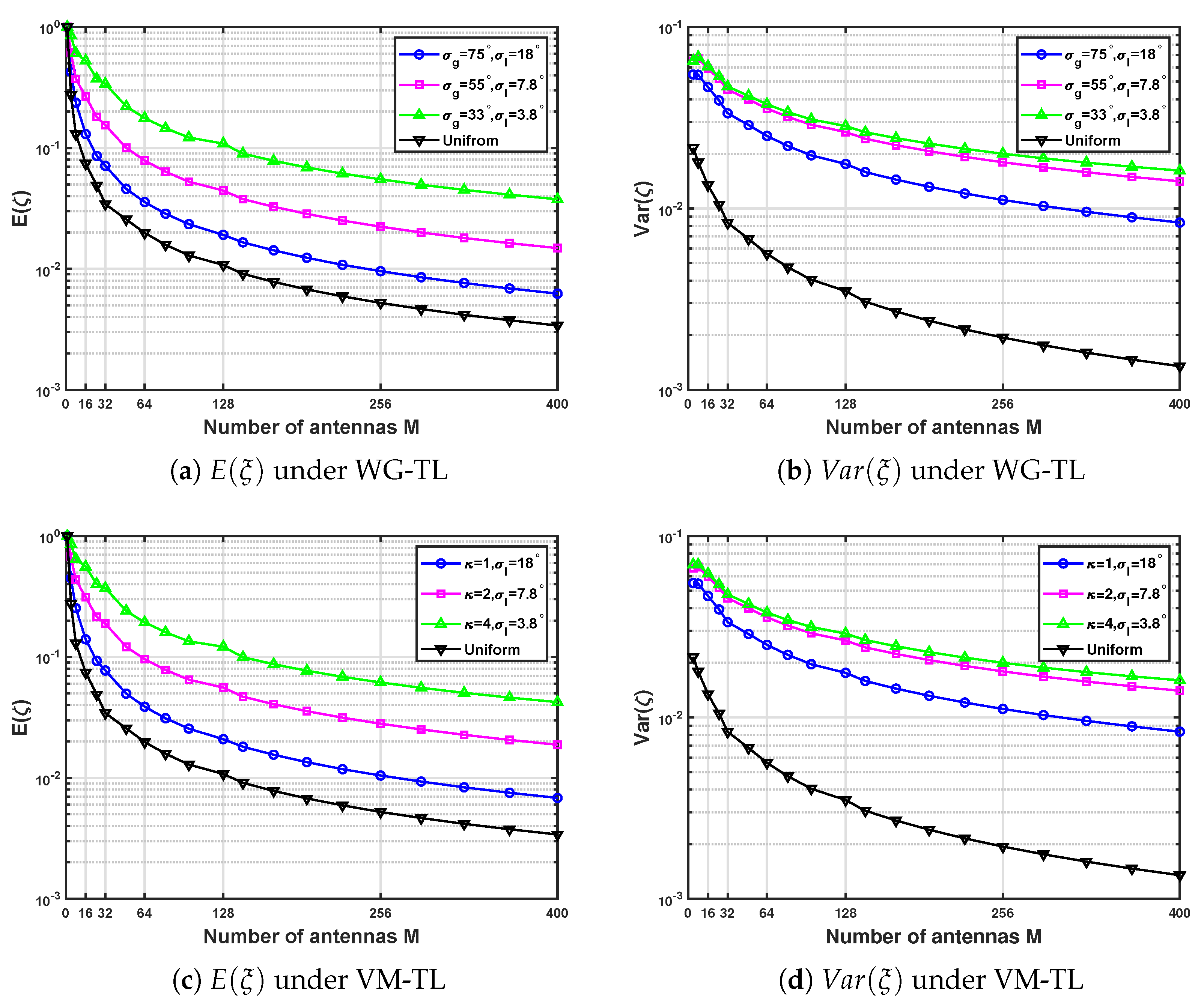
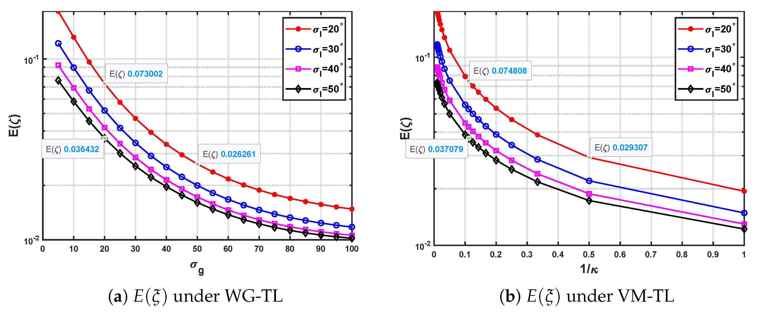
4.1. Statistical Property Analysis

This part analyzes the mathematical expressions of the expectations $E\left(\xi \right)$ and variances $Var\left(\xi \right)$ in Section 3.2. If not specified, UPA with half-wavelength antenna spacing is configured at BS. The configuration of the UPA element number is given in Table 3.

Table 3. The configuration of UPA elements in the horizontal and vertical dimensions.

Type	Element Number
Total	4	8	16	25	32	49	64	81	100	128	144	169	196	256	289	324	361	400
Horizontal	2	4	4	5	8	7	8	9	10	16	12	13	14	16	17	18	19	20
Vertical	2	2	4	5	4	7	8	9	10	8	12	13	14	16	17	18	19	20

Firstly, Figure 3 shows the simulation results of $E\left(\xi \right)$ and $Var\left(\xi \right)$ varying with the antenna number M under different angle spreads $\sigma$ in WG-TL and concentration factors $\kappa$ in VM-TL. It can be seen that the expectation and variance under WG-TL are very similar to them under VM-TL due to the similarity of their PDF curves with similar angle spreads.

Figure 3. Expectations and variances against the antenna number M, angle spread $\sigma$ and concentration factor $\kappa$ under WG-TL and VM-TL.

Furthermore, as the antenna number increases, the expectation and variance decrease to zero quickly. The values of $E\left(\xi \right)$ and $Var\left(\xi \right)$ decrease to ${10}^{-2}$, especially when the antenna number is larger than 128. This result is consistent with the theoretical derivation and analysis in Section 3.2. Therefore, the asymptotically FP condition can be satisfied in a practical massive MIMO system. Besides, larger angle spreads make $E\left(\xi \right)$ and $Var\left(\xi \right)$ become smaller. In this case, different spatial DoFs can be allocated to each user and the channel vectors of different users become orthogonal. For example, to achieve the expectation smaller than ${10}^{-1}$, the required number of antenna elements in ${\sigma }_g={78}^{\circ }$ and ${\sigma }_l={18}^{\circ }$, ${\sigma }_g={55}^{\circ }$ and ${\sigma }_l={7.8}^{\circ }$, ${\sigma }_g={33}^{\circ }$ and ${\sigma }_l={3.8}^{\circ }$ are about 25, 49 and 128, respectively. Moreover, the expectation and variance under the ideal uniform distributions decay to zero fastest due to its largest angle spread (${104}^{\circ }$ for the azimuth angle and ${52}^{\circ }$ for the elevation angle).

And then Figure 4 investigates the effects of elevation and azimuth angle spreads on $E\left(\xi \right)$ under WG-TL and VM-TL with the antenna number M=128. It can be seen that the declines of $E\left(\xi \right)$ caused by azimuth angle spreads are greater than those caused by elevation angle spreads. For example, when ${\sigma }_l$ increases from ${20}^{\circ }$ to ${50}^{\circ }$, $E\left(\xi \right)$ reduces about 0.037. However, when ${\sigma }_g$ increases from ${20}^{\circ }$ to ${50}^{\circ }$, $E\left(\xi \right)$ reduces about 0.047. The same phenomenon can be seen under VM-TL. The different angle distributions’ shapes can explain this. Compared with WG and VM, TL has the narrowest envelope, which makes the elevation AOAs more concentrated. The result implies that more antenna elements should be placed in the horizontal dimension to distinguish more azimuth angles.

Figure 4. Expectations against angle spreads under WG-TL and VM-TL with the antenna number M = 128.

Furtherly, Figure 5 shows the variations of $E\left(\xi \right)$ against antenna spacing under WG-TL and VM-TL with M=128, ${\sigma }_g={55}^{\circ }$, ${\sigma }_l={7.8}^{\circ }$, $\kappa =2$. For UPA, $d_{col}$ and $d_{row}$ represent the inter-element distance in the column and row, respectively. It is observed that $E\left(\xi \right)$ decreases quickly with the increase of $d_{col}$ and $d_{row}$. It implies that a larger distance between adjacent antenna elements can reduce inter-user interference. Besides, the values of $E\left(\xi \right)$ under the uniform distribution are the smallest due to the maximum angle spread, as observed in Figure 2. It is noted that the values of expectations decrease quickly with the increase of antenna spacing when the antenna spacing is smaller than $0.5\lambda$. However, the values of expectations hardly change when the Nyquist sampling rate in the spatial domain is satisfied [40], i.e., the antenna spacing is larger than $0.5\lambda$. This result is consistent with the theoretical analysis of holographic MIMO systems’ DoFs in [41], which means that the antenna aperture limits the holographic MIMO system performance. Larger antenna spacing with the same antenna number leads to a larger antenna aperture, which takes more DoFs. Therefore, setting the antenna spacing to about half-wavelength is a good choice when the antenna size and radiofrequency chain number are limited in the traditional engineering practice of MIMO systems.

Figure 5. Expectations against the antenna spacing under WG-TL and VM-TL with the antenna number M = 128.

Finally, Figure 6 investigates the effects of different antenna arrays on $E\left(\xi \right)$, where ${\sigma }_g={55}^{\circ }$, ${\sigma }_l={7.8}^{\circ }$, $\kappa =2$, $f_c=3.5$ GHz. It can be observed that the values of $E\left(\xi \right)$ under ULA are smaller than those under UPA with same antenna numbers. This result is because ULA has larger mean antenna spacing than UPA. However, the deployment of ULA in massive MIMO systems is unrealistic due to its large antenna aperture. For example, when the antenna number M is 128 and the antenna spacing is $0.5\lambda$, the antenna aperture of ULA is 10.88 m, which is about 7.5 times that of UPA. Besides, increasing the antenna number of UPA can achieve the same $E\left(\xi \right)$ as ULA but with smaller space. Thus, the deployment of UPA is a good choice for massive MIMO systems due to its compact size.

Figure 6. Expectations against the antenna number M under WG-TL and VM-TL with different antenna arrays.

4.2. Measures of the Favorable Propagation

Theoretical analysis and simulation results indicate that the asymptotically FP holds when the antenna number M tends to infinite. Nevertheless, the antenna number is always finite in reality. Therefore, we introduce two common metrics, i.e., the condition number (CN) and the distance from FP, to measure the proximity between the real channel and the channel under the FP condition in this part.

We define CN as the ratio between the largest and the smallest eigenvalues of the Gramian matrix ${\mathbf{G}}^H\mathbf{G}$ [5], i.e.,

$$CN=\frac{max\left\{Eigen\left({\mathbf{G}}^H\mathbf{G}\right)\right\}}{min\left\{Eigen\left({\mathbf{G}}^H\mathbf{G}\right)\right\}},$$

(27)

where $Eigen\left({\mathbf{G}}^H\mathbf{G}\right)$ represents the operation of calculating the eigenvalues of the matrix ${\mathbf{G}}^H\mathbf{G}$. Smaller CNs mean that the eigenvalues of ${\mathbf{G}}^H\mathbf{G}$ are more uniform, and they converge to one under the FP condition with equal large-scale fading $\beta$ for all users. In this case, different users’ channel vectors become orthogonal. CN is easy to be obtained with the utilization of $\mathbf{G}$. However, it has two drawbacks: (i) it only has a sound operational meaning with the same norm for all $\left\{{\mathbf{g}}_k\right\}$ and (ii) it disregards all other eigenvalues except for the maximum and minimum. Thus, we define the distance from FP, i.e.,

$$\mathrm{\Delta }C=\frac{{\displaystyle \sum _{k=1}^K}{log}_2(1+\rho {∥{\mathbf{g}}_k∥}_2^2)-{log}_{2}det({\mathbf{I}}_K+\rho {\mathbf{G}}^H\mathbf{G})}{{log}_{2}det({\mathbf{I}}_K+\rho {\mathbf{G}}^H\mathbf{G})}.$$

(28)

The distance from FP represents the capacity gap between the real channel and the channel under the FP condition. When $\mathrm{\Delta }C=0$, the channel satisfies the FP condition.

The system model in (1) is adopted to simulate the massive MIMO system capacity performance. In the simulation, six independent users are simultaneously served by one BS deployed with UPA. The transmit SNR is set to $\rho =0$ dB, and the large-scale fading $\beta$ is normalized to unit power.

In Figure 7, we compare CNs’ cumulative distribution functions (CDFs) for two specific scale antenna numbers in different scenarios. It can be seen that the 50% CDFs of 256-antenna massive MIMO systems are 8.2, 8.6, and 9.1 dB lower than those of 16-antenna MIMO systems in UMi, UMa, and RMa scenarios, respectively. Moreover, the CN distributions of 256-antenna massive MIMO systems are much more stable than those of 16-antenna MIMO systems. This result indicates that the channel vectors tend to be orthogonal and become hardening as the antenna number increases.

Figure 7. Condition numbers in UMi, UMa and RMa scenarios with different antenna configurations.

Besides, the CN values of UMi is the smallest, followed by UMa, and RMa is the largest for both 16 and 256-antenna MIMO systems. This result is because UMi has the richest scattering environment, which leads to the largest angle spread (although the inter-cluster angle spread is not the largest, the intracluster angle spread is the largest). On the contrary, RMa has the weakest scattering, which leads to the smallest angle spread. These results are consistent with the field measurements in [6,42], which furtherly validate our analysis. Also, it can be seen that uniform distributions have the smallest CN values compared with these three scenarios. This result is due to the assumption of ideal uniform rich-scattering propagation, and it overestimates the proximity between the real channel and the channel under the FP condition.

Furthermore, the expectations of $\left|\frac{1}{M}{\mathbf{g}}_i^H{\mathbf{g}}_j\right|$ in UMi, UMa, and RMa with different antenna configurations are given in Table 4. It is clearly that the values of $E\left(\left|\frac{1}{M}{\mathbf{g}}_i^H{\mathbf{g}}_j\right|\right)$ in the large-scale MIMO system are about 70% lower than those in the small-scale MIMO system. It implies that inter-user interference can be mitigated by increasing the antenna number. Moreover, we can find that larger angle spreads also decrease inter-user interference by comparing the values in different scenarios.

Table 4. Values of $E\left(\left|\frac{1}{M}{\mathbf{g}}_i^H{\mathbf{g}}_j\right|\right)$ in UMi, UMa and RMa with different antenna configurations.

Case	UMi-16	UMa-16	RMa-16	UMi-256	UMa-256	RMa-256
$E\left(\left|\frac{1}{M}{\mathbf{g}}_i^H{\mathbf{g}}_j\right|\right)$	0.2606	0.3101	0.3794	0.0775	0.0966	0.1034

Finally, Figure 8 shows the variations of the distance from FP against the antenna number M, angle spread $\sigma$ and concentration factor $\kappa$. Obviously, the distance from FP converges to zero quickly as the antenna number increases. This result implies that the capacity of massive MIMO systems can approach the maximum capacity obtained under the FP condition if the antenna number is large enough. Besides, we can investigate the capacity performance in different scattering environments by tuning the WG, TL, and VM parameters, i.e., ${\sigma }_g$, and ${\sigma }_l$, and $\kappa$. It is observed that the FP condition is easier to be satisfied in the rich scattering environment. Moreover, we plot the average capacity ratios between the real channel under three scenarios and i.i.d. Rayleigh channels with the increase of antenna numbers. It can be seen that the capacity achieved in real scenarios reaches more than 90% of that of i.i.d. Rayleigh channels when the antenna number is ten times the number of users, i.e., 64.

Figure 8. The distance from FP against the antenna number M, angle spread $\sigma$ and concentration factor $\kappa$ under WG-TL and VM-TL.

5. Measurement Validation

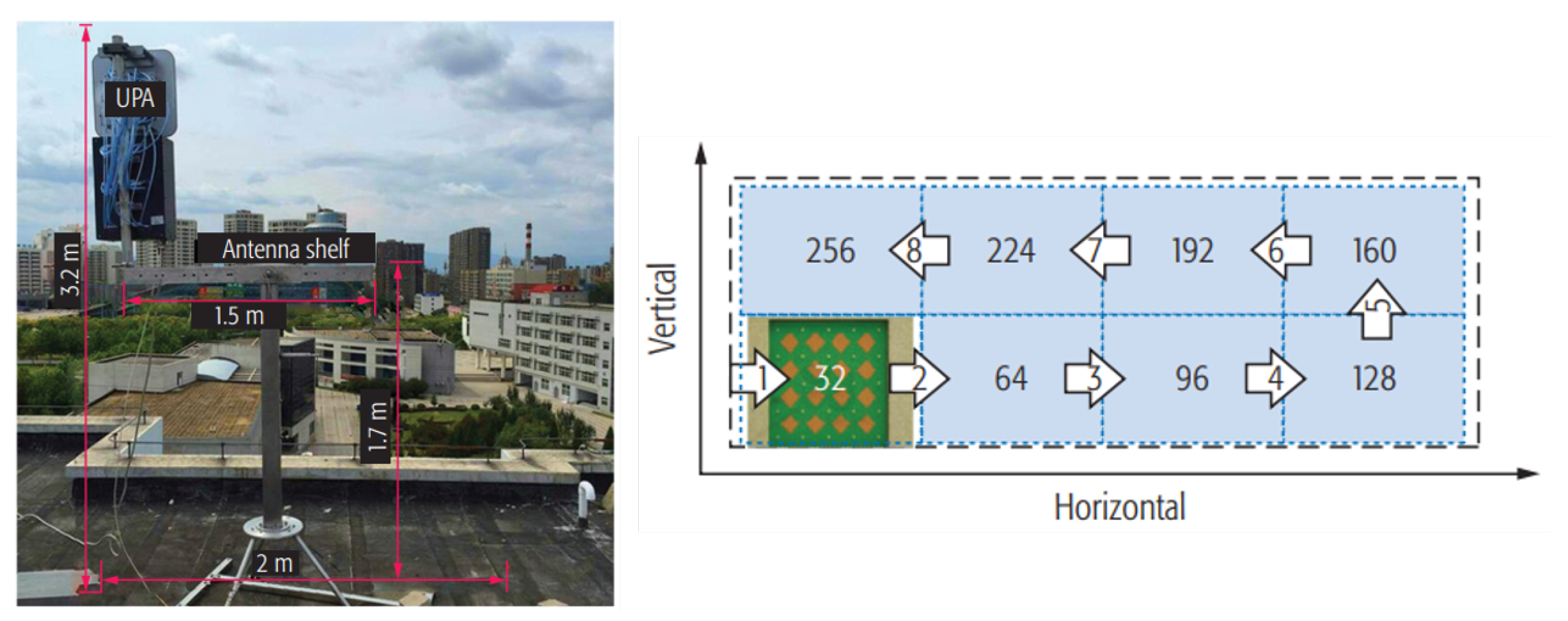
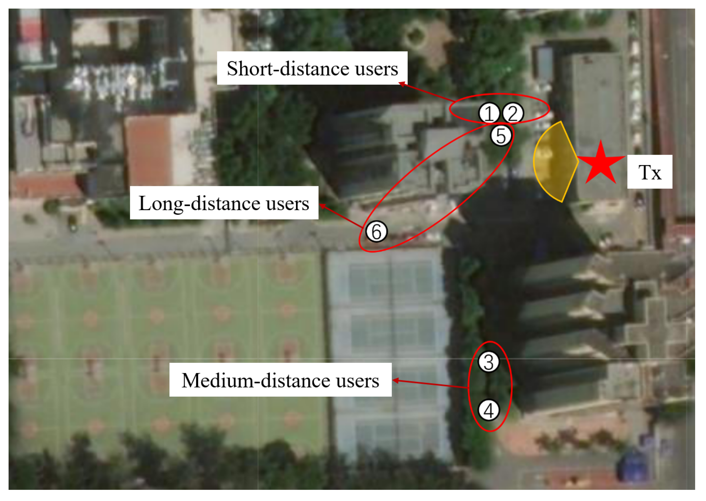
5.1. Measurement Description

To validate the experimental FP condition, we conducted channel measurements in an urban micro scenario [6]. Elektrobit Propsound channel sounder was adopted to obtain the 3D massive MIMO channel impulse response at the 3.5 GHz frequency band. A UPA with 32 elements and an omnidirectional array (ODA) with 56 elements were used to transmit and receive the channel-sounding signal. The UPA was vertically and horizontally shifted in a specific mechanical metal shelf in Figure 9 to realize the 256 antenna elements’ massive MIMO channel measurement. In our analysis, we select 4, 8, 16, 32, 64, 128, and 256 Tx elements from the shifted composite UPA to analyze the FP condition with the antenna number varying and choose one Rx element with the largest received power in the ODA as the user’s received antenna. Other detailed measurement system configurations and information are given in [6]. As shown in Figure 10, the transmitter was installed on the top of a 12-meter building and towards the west. Six measurement positions are selected and divided into three groups, which represent two users with 1.7 meter-short, 14 meter-medium and 41 meter-long distance between each other.

Figure 9. The antenna shelf and massive MIMO measurement principle diagram of 3D MIMO antennas from 32 to 256 at Tx [6].

Figure 10. The top view of a practical urban micro measurement scenario from Baidu satellite map.

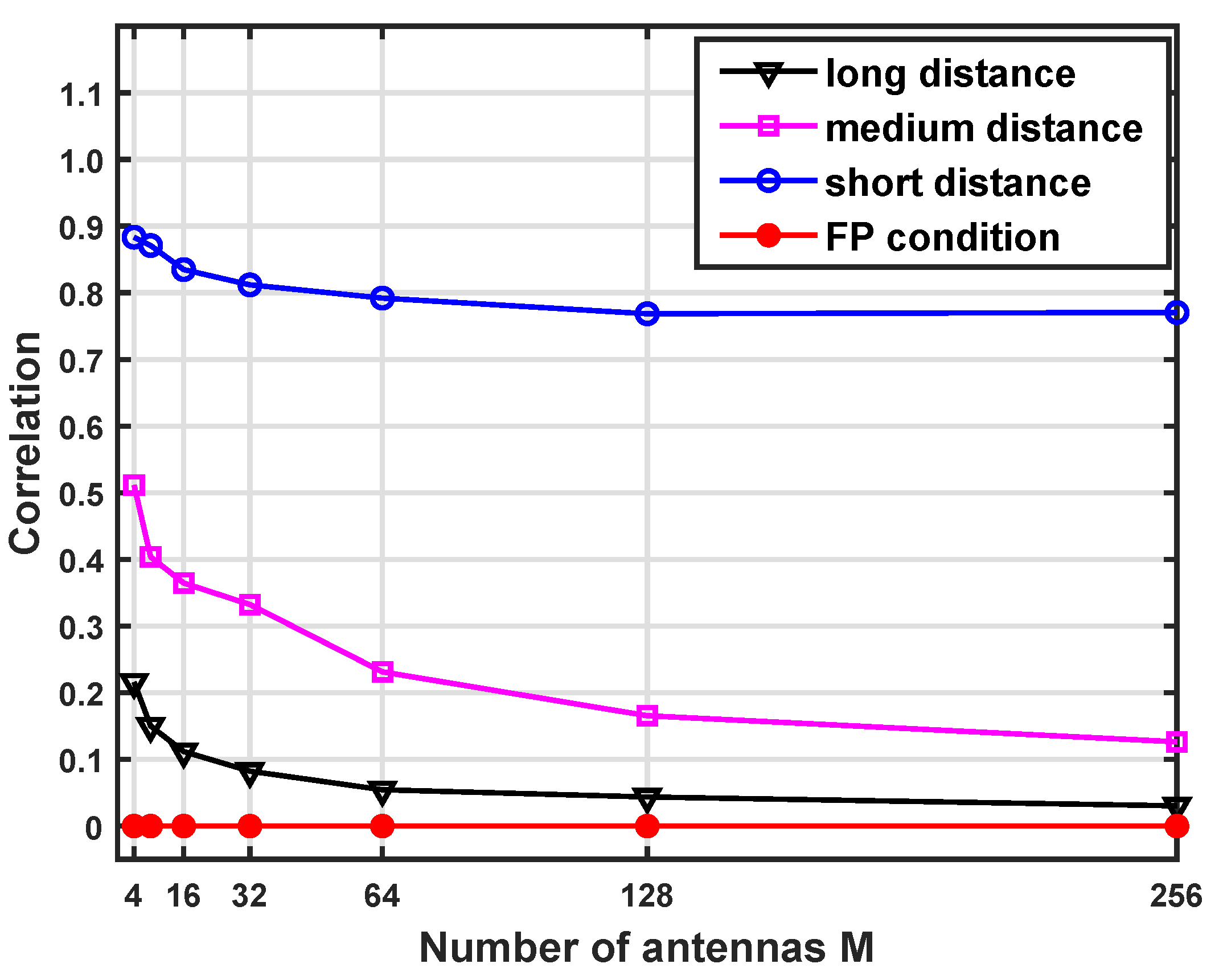
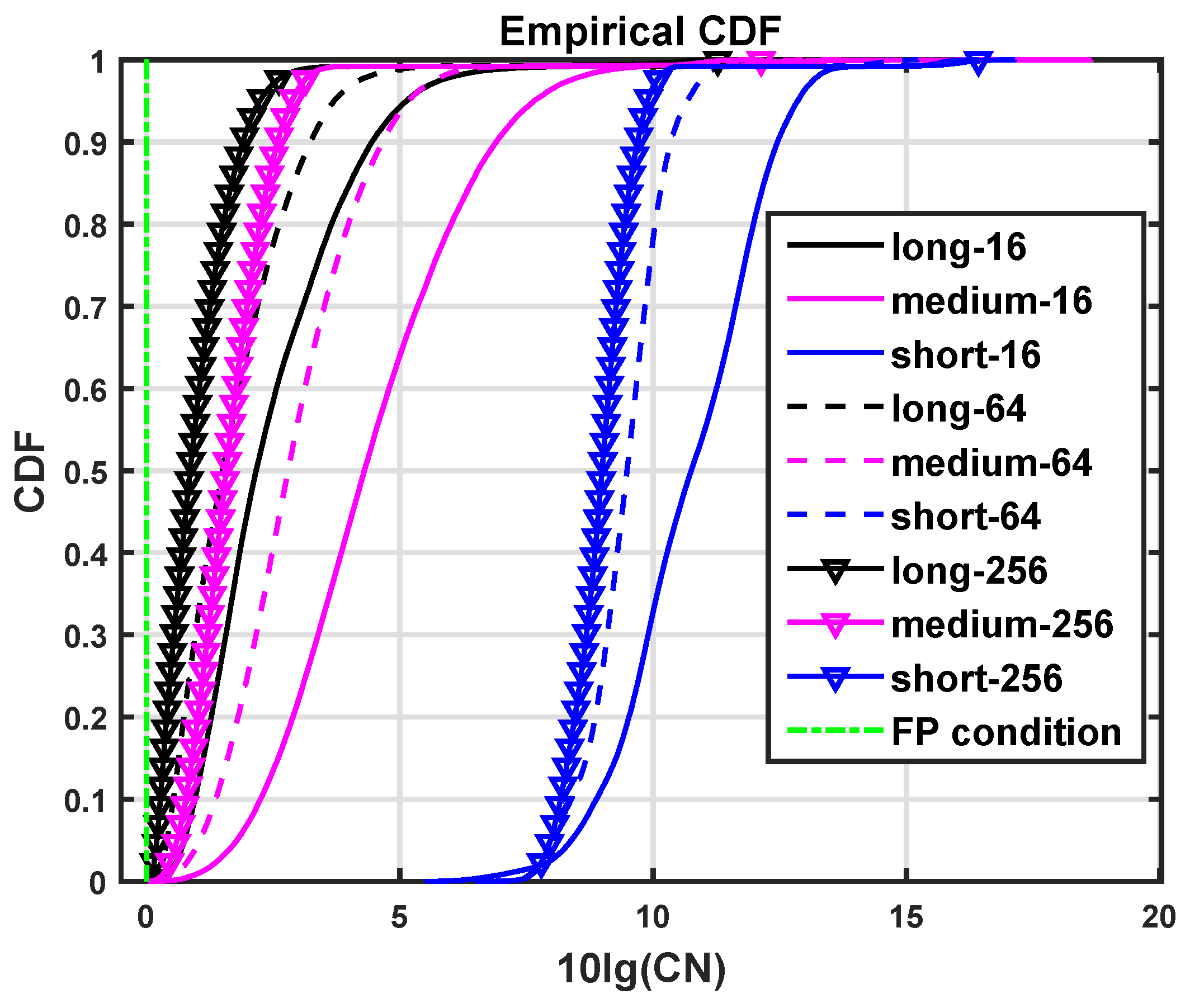
5.2. Result Analysis

Firstly, Figure 11 and Figure 12 show the results of channel correlations and CNs with antenna numbers in the practical measurement scenario, respectively. They are calculated by (3) and (27), respectively. The channel correlations and the CNs increase with the users close to each other. As the antenna number increases from 4 to 256, the correlations decrease by about 12.8%, 75.3%, and 85.9% in the short, medium, and long-distance, respectively. When the users are far away from each other, the correlations tend to be zero, and the CNs are nearly one in the 256-antenna case. These results are consistent with the theoretical analysis and numerical simulations, which means different users’ channel vectors become orthogonal in this case.

Figure 11. Channel correlations in a practical measurement scenario with different antenna configurations.

Figure 12. Condition numbers in a practical measurement scenario with different antenna configurations.

Moreover, Figure 13 shows the distance from the FP condition and the capacity ratio of the real channels to i.i.d. Rayleigh channels against antenna numbers in the practical scenario. The distance is calculated by (28). It can be seen that the distance from FP becomes smaller, and the capacity ratio rises with the antenna number increasing. When the antenna number is less than 32, the distances from FP are about 22.9%, 5.8%, and 1.1% in the short, medium, and long-distance between users, respectively. The real channel capacity of two long-distance users is very close to Rayleigh channels, especially in the 256-antenna case. This result is due to the significant differences in propagation environment between the two long-distance users. The FP condition is easy to realize as the antenna number tends to infinity. The theoretical proof in Section 3 can well explain these phenomena and evaluate the FP’s performance in any scenarios.

Figure 13. The distance from FP in a practical measurement scenario with different antenna configurations.

6. Conclusions

This paper investigates the asymptotically FP condition of a 3D MIMO channel under the assumption of generalized angle distributions, i.e., WG-TL and VM-TL. Theoretical analysis proves that the asymptotically FP is satisfied under these distributions, and the FP condition is easier to be satisfied in rich scattering environments. Besides, the effect of azimuth angle spreads on FP is more significant than that of elevation angle spreads due to different angle distributions in the spatial horizontal and vertical domains. In addition, the antenna aperture limits the system performance. Larger antenna spacing with the same antenna number leads to smaller inter-user interference. Hence, using compact antenna arrays, such as UPA, and setting antenna spacing as about half-wavelength are good choices when the antenna size is limited in engineering practice. Moreover, we have proved that the uniform distribution is a particular case of the generalized angle distributions. And the capacity achieved in real scenarios can reach more than 90% of the i.i.d. Rayleigh channel capacity when the antenna number is ten times the number of users. Finally, it has been shown that the channel vectors of users in more diverse propagation environments are easier to meet the FP condition. In the future, we will extend our research to more generalized near-field cases when the antenna size is non-negligible compared with the distance between BSs and users. In these cases, the spatial non-stationary will be considered in our analysis.

References

- IMT Vision-Framework and Overall Objectives of the Future Development of IMT for 2020 and Beyond; International Telecommunication Union: New York, NY, USA, 2015.
- Tataria, H.; Shafi, M.; Molish, A.F.; Dohler, M.; Sjöland, H.; Tufvesson, F. 6G wireless systems: Vision, requirements, challenges, insights, and opportunities. Proc. IEEE 2021, 109, 1166–1199. [Google Scholar] [CrossRef]
- Agbotiname, L.I.; Oluwadara, A.; Nistha, T.; Sachin, S. 6G Enabled Smart Infrastructure for Sustainable Society: Opportunities, Challenges, and Research Roadmap. Sensors 2021, 21, 1709. [Google Scholar]
- Marzetta, T.L. Noncooperative Cellular Wireless with Unlimited Numbers of Base Station Antennas. IEEE Trans. Wirel. Commun. 2010, 9, 3590–3600. [Google Scholar] [CrossRef]
- Zhang, J.; Zhang, Y.; Yu, Y.; Xu, R.; Zheng, Q.; Zhang, P. 3-D MIMO: How Much Does It Meet Our Expectations Observed From Channel Measurements? IEEE J. Select. Areas Commun. 2017, 35, 1887–1903. [Google Scholar] [CrossRef]
- Zhang, J.; Zheng, Z.; Zhang, Y.; Xi, J.; Zhao, X.; Gui, G. 3D MIMO for 5G NR: Several Observations from 32 to Massive 256 Antennas Based on Channel Measurement. IEEE Commun. Mag. 2018, 56, 62–70. [Google Scholar] [CrossRef]
- Rusek, F.; Persson, D.; Lau, B.K.; Larsson, E.G.; Marzetta, T.L.; Edfors, O.; Tufvesson, F. Scaling up MIMO: Opportunities and challenges with very large arrays. IEEE Sign. Process. Mag. 2013, 30, 40–60. [Google Scholar] [CrossRef] [Green Version]
- Borges, D.; Montezuma, P.; Dinis, R.; Beko, M. Massive MIMO Techniques for 5G and beyond opportunities and Challenges. Electronics 2021, 10, 1667. [Google Scholar] [CrossRef]
- Zhang, M.; Tan, L.; Huang, K.; You, L. On the Trade-Off between Energy Efficiency and Spectral Efficiency in RIS-Aided Multi-User MISO Downlink. Electronics 2021, 10, 1307. [Google Scholar] [CrossRef]
- Zhang, J.; Pan, C.; Pei, F.; Liu, G.; Cheng, X. Three-dimensional fading channel models: A survey of elevation angle research. IEEE Commun. Mag. 2014, 52, 218–226. [Google Scholar] [CrossRef]
- Yu, Y.; Zhang, J.; Smith, P.J.; Dmochowski, P.A. Theoretical Analysis of 3-D Channel Spatial Correlation and Capacity. IEEE Commun. Lett. 2018, 22, 420–423. [Google Scholar] [CrossRef]
- Yu, Y.; Smith, P.J.; Dmochowski, P.A.; Zhang, J.; Shafi, M. 3D vs. 2D channel models: Spatial correlation and channel capacity comparison and analysis. In Proceedings of the 2017 IEEE International Conference on Communications (ICC), Paris, France, 21–25 May 2017; pp. 1–7.
- Nam, Y.; Ng, B.L.; Sayana, K.; Li, Y.; Zhang, J.; Kim, Y.; Lee, J. Full-dimension MIMO (FD-MIMO) for next generation cellular technology. IEEE Commun. Mag. 2013, 51, 172–179. [Google Scholar] [CrossRef]
- Pizzo, A.; Marzetta, T.L.; Sanguinetti, L. Spatially-stationary model for holographic MIMO small-scale fading. IEEE J. Select. Areas Commun. 2020, 38, 1964–1979. [Google Scholar] [CrossRef]
- Pizzo, A.; Sanguinetti, L.; Marzetta, T.L. Fourier Plane-Wave Series Expansion for Holographic MIMO Communications. IEEE Trans. Wirel. Commun. 2022, 1. [Google Scholar] [CrossRef]
- Sun, Y.; Tian, L.; Zhang, J.; Wu, L.; Zhang, P. On asymptotic favorable propagation condition for massive MIMO with co-located user terminals. In Proceedings of the 2014 International Symposium on Wireless Personal Multimedia Communications (WPMC), Sydney, Austrlia, 7–10 September 2014; pp. 706–711. [Google Scholar]
- Zhang, J.; Zhang, J.; Tian, L.; Xu, R.; Zhang, Z. Favorable Propagation with Practical Angle Distributions for mm Wave Massive MIMO Systems. In Proceedings of the 2019 IEEE International Conference on Communications Workshops (ICC Workshops), Shanghai, China, 20–24 May 2019; pp. 1–6. [Google Scholar]
- Ngo, H.Q.; Larsson, E.G.; Marzetta, T.L. Aspects of favorable propagation in Massive MIMO. In Proceedings of the 2014 22nd European Signal Processing Conference (EUSIPCO), Lisbon, Portugal, 1–5 September 2014; pp. 76–80. [Google Scholar]
- Papazafeiropoulos, A.; PaKourtessis, P.; Renzo, M.D.; Chatzinotas, S.; Senior, J.M. Performance Analysis of Cell-Free Massive MIMO Systems: A Stochastic Geometry Approach. IEEE Trans. Veh. Technol. 2020, 69, 3523–3537. [Google Scholar] [CrossRef] [Green Version]
- Chien, T.V.; Ngo, H.Q.; Chatzinotas, S.; Ottersten, B. Reconfigurable Intelligent Surface-Assisted Massive MIMO: Favorable propagation, channel hardening, and rank deficiency. IEEE Sign. Process. Mag. 2022, 39, 97–104. [Google Scholar] [CrossRef]
- Wu, X.; Beaulieu, N.C.; Liu, D. On Favorable Propagation in Massive MIMO Systems and Different Antenna Configurations. IEEE Access 2017, 5, 5578–5593. [Google Scholar] [CrossRef]
- Cai, W.; Wang, P.; Li, Y.; Zhang, Y.; Pan, P. Asymptotic Capacity Analysis for Sparse Multipath Multiple-Input Multiple-Output Channels. IEEE Commun. Lett. 2015, 19, 2262–2265. [Google Scholar] [CrossRef]
- Kebede, T.; Wondie, Y.; Steinbrunn, J. Channel Estimation and Beamforming Techniques for mm Wave-Massive MIMO: Recent Trends, Challenges and Open Issues. In Proceedings of the 2021 International Symposium on Networks, Computers and Communications (ISNCC), Abu Dhabi, Dubai, 1–3 June 2021. [Google Scholar]
- Shafi, M.; Zhang, J.; Tataria, H.; Molisch, A.F.; Sun, S.; Rappaport, T.S.; Tufvesson, F.; Wu, S.; Kitao, K. Microwave vs. Millimeter-Wave Propagation Channels: Key Differences and Impact on 5G Cellular Systems. IEEE Commun. Mag. 2018, 56, 14–20. [Google Scholar] [CrossRef]
- Yoo, J.; Sung, W.; Kim, I. 2D-OPC Subarray Structure for Efficient Hybrid Beamforming over Sparse mmWave Channels. Int. J. Antennas Propag. 2021, 2021, 6680566. [Google Scholar] [CrossRef]
- Pratschner, S.; Blazek, T.; Groll, H.; Caban, S.; Schwarz, S.; Rupp, M. Measured User Correlation in Outdoor-to-Indoor Massive MIMO Scenarios. IEEE Access 2020, 8, 178269–178282. [Google Scholar] [CrossRef]
- Gao, X.; Edfors, O.; Rusek, F.; Tufvesson, F. Massive MIMO Performance Evaluation Based on Measured Propagation Data. IEEE Trans. Wirel. Commun. 2015, 14, 3899–3911. [Google Scholar] [CrossRef] [Green Version]
- Guevara, A.P.; Bast, S.D.; Pollin, S. Massive MIMO: A Measurement-Based Analysis of MR Power Distribution. In Proceedings of the 2020 IEEE Global Communications Conference, Taipei, Taiwan, 7–11 December 2020. [Google Scholar]
- I-METRA D2: Channel Characterisation; Information Society Technologies: New York, NY, USA, 2012.
- Ampoma, A.E.; Wen, G.; Zhang, H.; Huang, Y.; Gyasi, O.K.; Tebe, P.I. 3D correlation function of a uniform circular array using maximum power in the direction of arrival. In Proceedings of the 2017 Progress in Electromagnetics Research Symposium-Fall (PIERS-FALL), Singapore, 19–22 November 2017; pp. 2996–3003. [Google Scholar]
- Nadeem, Q.; Kammoun, A.; Debbah, M.; Alouini, M. A Generalized Spatial Correlation Model for 3D MIMO Channels Based on the Fourier Coefficients of Power Spectrums. IEEE Trans. Sign. Process. 2015, 63, 3671–3686. [Google Scholar] [CrossRef] [Green Version]
- Ampoma, A.E.; Wen, G.; Huang, Y.; Gyasi, K.O.; Tebe, P.I.; Ntiamoah-Sarpong, K. Spatial Correlation Models of Large-Scale Antenna Topologies Using Maximum Power of Offset Distribution and its Application. IEEE Access 2018, 6, 36295–36304. [Google Scholar] [CrossRef]
- Queiroz, W.J.; Madeiro, F.; Lopes, W.T.A.; Alencar, M.S. Spatial Correlation for DoA Characterization Using Von Mises, Cosine, and Gaussian Distributions. Int. J. Antennas Propag. 2011, 2011, 540275. [Google Scholar] [CrossRef]
- Study on Channel Model for Frequency from 0.5 to 100 GHz (Release 14). 2017. Available online: http://www.3gpp.org/ (accessed on 30 May 2022).
- Guidelines for Evaluation of Radio Interface Technologies for IMT-2020; Information Society Technologies: New York, NY, USA, 2017.
- Li, Y.; Zhang, J.; He, R.; Tian, L.; Wei, H. Hybrid DE-EM Algorithm for Gaussian Mixture Model-Based Wireless Channel Multipath Clustering. Int. J. Antennas Propag. 2019, 2019, 4639612. [Google Scholar] [CrossRef]
- Temiz, M.; Alsusa, E.; Danoon, L.; Zhang, Y. On the Impact of Antenna Array Geometry on Indoor Wideband Massive MIMO Networks. IEEE Trans. Antennas Propag. 2020, 69, 406–416. [Google Scholar] [CrossRef]
- Lindgren, B. Statistical Theory; Routledge: London, UK, 2017. [Google Scholar]
- Abramowitz, M.; Stegun, I.A. Handbook of Mathematical Functions with Formulas, Graphs and Mathematical Tables; Dover: New York, NY, USA, 1970. [Google Scholar]
- Tse, D.; Viswanath, P. Fundamentals of Wireless Communications; Cambridge University Press: Cambridge, UK, 2005. [Google Scholar]
- Pizzo, A.; Marzetta, T.L.; Sanguinetti, L. Degrees of freedom of holographic MIMO channels. In Proceedings of the 2020 IEEE 21st International Workshop on Signal Processing Advances in Wireless Communications (SPAWC), Online, 26–29 May 2020. [Google Scholar]
- Neil, C.T.; Shafi, M.; Smith, P.J.; Dmochowski, P.A.; Zhang, J. Impact of Microwave and mmWave Channel Models on 5G Systems Performance. IEEE Trans. Antennas Propag. 2017, 65, 6505–6520. [Google Scholar] [CrossRef]
- Gradshteyn, I.S.; Ryzhik, I.M. Table of Integrals, Series, and Products, 7th ed.; Academic Press: Cambridge, MA, USA, 2014. [Google Scholar]
Publisher’s Note: MDPI stays neutral with regard to jurisdictional claims in published maps and institutional affiliations. |
© 2022 by the authors. Licensee MDPI, Basel, Switzerland. This article is an open access article distributed under the terms and conditions of the Creative Commons Attribution (CC BY) license (https://creativecommons.org/licenses/by/4.0/).