Abstract
Massive MIMO technology is among the most promising solutions for achieving higher gain in 5G millimeter-wave (mmWave) channel models for high-speed train (HST) communication systems. Based on stochastic geometry methods, it is fundamental to accurately develop the associated MIMO channel model to access system performance. These MIMO channel models could be extended to massive MIMO with antenna arrays in more than one plane. In this paper, the proposed MIMO 3D geometry-based stochastic model (GBSM) is composed of the line of sight component (LOS), one sphere, and multiple confocal elliptic cylinders. By considering the proposed GBSM, the local channel statistical properties are derived and investigated. The impacts of the distance between the confocal points of the elliptic cylinder, mmWave frequencies of 28 GHz and 60 GHz, and non-stationarity on channel statistics are studied. Results show that the proposed 3D simulation model closely approximates the measured results in terms of stationary time. Consequently, findings show that the proposed 3D non-wide-sense stationary (WSS) model is better for describing mmWave HST channels in an open space environment.
1. Introduction
High-speed Trains with a speed of 500 km/h and above are particularly expected to be supported in the fifth-generation 5G wireless mobile communication [1]. China’s CIT500 train has been recorded as the fastest at 605 km/h while the Maglev train of Japan is the second fastest at 603 km/h. In such a situation, there is high demand for conditions to satisfy passenger needs as well as safety for the train during communication. In this case, channel modeling for 5G using mmWave bands in the HST communication system is required [2]. The exact challenges usually come from very fast hand over, which sometimes worsens the situation when the vehicle is moving through different scattering environments [3].
Previously, the Global System for Mobile Communication Railway (GSM-R), which could only provide a maximum 200 kbps data rate, was implemented in the European Train Control System (ETCS) in 1998; however, this was mainly used more in the control system rather than providing train passengers mobile communication [3]. Because of the lower data rate, the International Union of Railways later recommended a 4G LTE-R, which is a broadband wireless communication system (4G) [4]. Although LTE-R is expected to deliver higher data rates than GSM-R, it still uses the original GSM-R mobile architecture of the mobile station user communicating directly to the base station user. Using this architecture for very high-speed trains leads to a low quality of service. This is basically due to fast-changing channels at the mobile radio station (MRS) onboard which increases the chances of handover failure [3]. Therefore, since there is a rapid development of very fast trains, especially in Maglev, there is a need for a high-quality wireless communication channel with high data rates for smart railway transport [4]. Thus, academia and the telecommunication industry have collaborated on the development, testing, and deployment of innovative wireless communication systems [5]. With smart rail transport, the passengers will be able to have a reliable, high-capacity communication channel that can handle applications such as video streaming in real-time-variantwithout interruptions regardless of the speed and location of the train. To obtain a channel that can handle the needs of a high-speed train, 5G and beyond mobile technology should be applied [5].
For the development of a 5G mmWave High-speed train communication system as showm in Figure 1, it is necessary to understand the underlying propagation channel, since different propagation distances and varying frequencies are mainly limited by pathloss [6]. For example, the case of [7,8,9] proposed how to reduce the likelihood of communication outages using MIMO technology that was integrated with different schemes for mobile communications. The shortcomings of short wavelength, high attenuation, atmospheric attenuation, precipitation attenuation, and absorption loss define mmWave frequency transmission. The use of high-gain antennas through massive MIMO technology helps mitigate the effects of the atmosphere and precipitation. In addition, massive MIMO technology in mmWave bands for HST communication helps to achieve long-distance transmission [10]. This helps to reduce handover frequency because the separation between base stations is kept large.
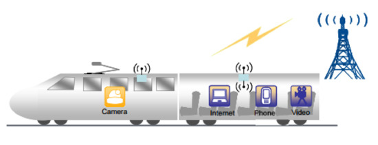
Figure 1.
A 5G HST communication system architecture with mobile MRS as in [1].
On the other hand, the channel characteristics can be described by modeling the HST multipath channel for different environments. Aside from geometry-based models, the 5G mmWave HST multipath propagation channel model can be exploited effectively through the ray tracing method [11]. The approach approximates well-measured results, although it has a high computation complexity; therefore, the modeling of real HST multipath fading channels using geometry-based models has been receiving more and more attention, such as [12,13,14,15,16,17,18,19,20]. In [13], a novel three-dimensional (3D) wideband MIMO HST RS-GBSM for non-isotropic scattering Rician fading channels was proposed—the same concept could be applied in HST channel modeling; however, mmWave frequencies were not considered. In addition, the underlying 5G HST channels exhibit frequency selectivity since the signal bandwidth is larger than or in the order of the coherence bandwidth (normally 4–6 MHz) [15]. As a result, mmWave frequency channel models need to be investigated.
In the literature, the wide-sense stationary (WSS) assumption was used in HST channel models. These WSS channel modeling approaches can be categorized into deterministic and stochastic approaches [13]. Under the stochastic approach, these can be further classified as the geometry-based stochastic model and non-geometry-based stochastic model [16]. Furthermore, GBSMs can be classified as regular-shaped GBSMs (RS-GBSMs) and irregular-shaped GBSMs (IS-GBSMs) [17,18], depending on whether effective scatterers are located on regular shapes, e.g., one ring, two-ring, ellipses, or irregular shapes. The WSS HST channel models in [17,19] assumed that multipath channel statistics characteristics are constant with respect to time. After taking the HST experimental channel measurements as shown in [20], it was concluded that the channel is only stationary for an interval time of milliseconds. For this reason, researchers have been motivated to re-evaluate the WSS assumption on HST channels by applying different approaches. The idea of the local scattering function (LSF) was first developed in [21] to characterize channels as non-stationary. The non-WSS channel model for generalized narrowband MIMO was introduced in [22] and yet mmWave frequencies are supposed to be wideband since they have a large bandwidth. Furthermore, the effect of a wideband non-stationary HST channel on channel capacity discussed in [23] did not consider mmWave frequencies. The 3D HST GBSMs were proposed in [13] considered multiple confocal ellipsoid geometry. In this research, a sphere was introduced around the MRS to represent uniformly distributed scatterers. This was performed because they are mainly affected by reflection. Although channel measurements path loss analysis has been analyzed in [24,25], no GBSM channel model has been built. Although channel measurements for mmWave frequencies were made in [25,26], the study in [25] exhibited characteristics of voltage amplitudes following a Rician distribution; therefore, the Rician distribution will be assumed in the model. In addition, it is important to evaluate the stationary interval. This describes the maximum length of time in which the correlation of channel coefficient exceeds the predefined threshold. These characteristics at mmWave frequencies have been analyzed using a ray tracing simulation in [27]; however, these have high computational complexity. As a train traverses the BS multipath components change causing varying signal power [28]. For that reason, channel characteristics with different frequencies have to be explored and the definitions of parameters used in the derivation are listed in Table 1.

Table 1.
Definition of parameters.
The main contributions of this work are
- 1.
- A generic GBSM 3D non-stationary wideband channel consisting of one sphere and multiple confocal elliptic cylinders is proposed as well as deriving the theoretical and simulation channel properties.
- 2.
- By considering mmWave carrier frequencies for the HST communication channel, the time-variant cross-correlation function (CCF), autocorrelation function (ACF), and the level crossing rate (LCR) are derived and studied thoroughly.
- 3.
- The impact of mmWave frequencies, non-stationarity, and the distance between the mobile radio station (MRS) and base station (BS) on channel statistics are investigated.
- 4.
- The applicability of the proposed model is verified by comparing it with measured data.
2. 3D Wideband Non-Stationary MIMO HST Theoretical Channel Model
The HST propagation channel model using the 3D wideband GBSM approach is presented as shown in Figure 2. The system consists of omni-directional U transmits and S receive antenna elements. A matrix is used to describe the fading channel. The proposed 3D wideband HST MIMO channel is demonstrated in Figure 2. The model considers LOS components and a single bounce component. In the HST channel model, the impact on channel statistics is considered for an open space environment. As illustrated in Figure 2, we employed the GBSM consisting of one-sphere and many confocal elliptic cylinders representing the stationary and uniformly distributed scatterers and the non-stationary environment situations, respectively. Figure 2 shows the detailed geometry. Based on the time delay line concept, the complex space time-variant channel impulse response of a MIMO channel model between the element of the base station, and the element of the moving receiver station is derived as summarized in Algorithm 1 channel simulation modeling and can be expressed as in (1) from [15]. Although only azimuth angles were considered, this derivation is extended to 3D geometry.
where the tap number is represented by the subscript l while represents the total number of taps. The and represent the complex time-variant tap coefficients and the discrete propagation delay of the lth tap, respectively; therefore, is a narrowband and for easier analysis of the MIMO channel, will be used. Since the channel has been modeled in 3D, the antenna array configuration could be extended to massive MIMO in different plane such as cylindrical or spherical, which makes the signal radiation more practical.
| Algorithm 1 Channel Simulation modeling |
|
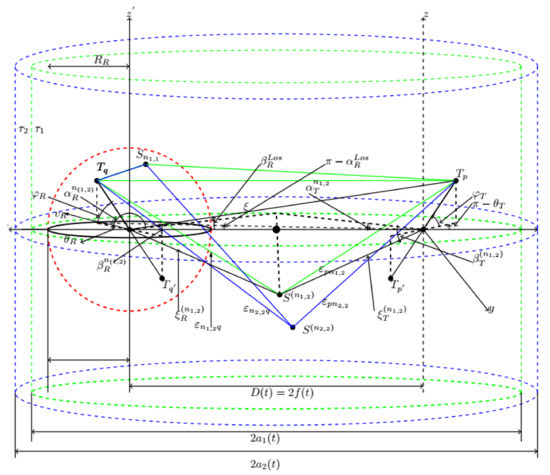
Figure 2.
Proposed GBSM for one sphere and multiple elliptic cylinder model. Green solid represents tap one, blue solid represents tap two, and red dash represent the MRS sphere.
2.1. First Tap
For the first tap, we suppose that around the sphere with radius , receiver Rx is located in the middle. There are scatterers on the sphere whereas an effective scatterer is defined by . The time delay structure with effective scatterers is represented by the multiple confocal elliptic-cylinder models consisting of at transmitter Tx and Rx at the two foci, respectively. The scatterers are located on the lth elliptic cylinder where . represents the time-variant total number of taps. There are scatterers on the semi major axis of the lth elliptic cylinder whereas the effective scatterer is defined by . The Tx and Rx antenna element spacing are denoted by and respectively. The half length distance between the foci of the ellipse is denoted by f; therefore, represents the distance D between the Tx and Rx. In this theoretical model, some assumptions such as min max, , and have been used; therefore, from the equation,
where,
We have time-varying parameters and , which make the underlying GBSM a non-stationary one. The designates the mean power for the lth tap, , and links → and →→, respectively. In Figure 2 there is one single-bounced component in the first tap, i.e., . The K and c represent the Rician factor and speed of light, respectively. Energy-related parameters specify how much the single bounced rays contribute to the total scattered power of the first tap. Note that these energy-related parameters are normalized to satisfy .
2.2. Other Taps
For other taps, the complex tap coefficients of only SB components make up the link →, which may be written as,
where is the time it takes for waves to travel via the link . Again, energy-related parameter indicate how much the SB rays contribute to the overall scattered power of other taps and it satisfies . The phases and , i.e., random variables with uniform distributions over while is the maximum Doppler frequency with respect to the MRS. In summary, the SB rays are generated from the scatterers on either the sphere or the first elliptic cylinder for the first tap. The LOS components, a sphere model with SB rays, and several confocal elliptic-cylinder models with SB rays are found in the first tap as shown in Figure 2. For additional taps, the SB rays components are assumed to be generated from the scatterers located on the corresponding elliptic cylinder. The underlying assumptions are based on the application of the law of cosines in triangles (i.e., and for small x), deducing min max, and we have,
where , , , , , , , and with denoting the semi-minor axis of the lth elliptic cylinder. Note that the Azimuth AoD (AAoD)/Elevation AoD(EAoD), (i.e., ) and Azimuth AoA (AAoA)/Elevation AoA(EAoA), (i.e., ), are correlated for SB rays. From the sphere model, we can derive the following relationship between the AoDs and AoAs of the SB rays: , . The angular relationships for SB rays derived from the elliptic-cylinder model are: and hold with denoting the semi axis of the lth elliptic cylinder. The discrete AAoD is used in the proposed theoretical 3D GBSM as the number of scatterers approaches infinity. , EAoD , AAoA and EAoA are replaced by continuous random variables , , , and , respectively, to consider the effects of azimuth and elevation angles on channel statistics simultaneously. In addition, to characterize the distribution of effective scatterers, we employ the von Mises–Fisher (VMF) probability density function (PDF), which was described in [29]
where ,, account for the mean values of the azimuth angle and the elevation angle , respectively, and is a real valued parameter that controls the concentration of the distribution as identified by the mean direction and ; in this case, for angular descriptions, i.e., the AAoA and EAoA for the sphere and the AAoA and EAoA for the multiple elliptic cylinders, the parameters ( and k) of the VMF PDF in and and and respectively.
2.3. Time-Varying Parameters
2.3.1. Total Number of Taps
To satisfy the non-stationary condition, the survival and death process is used in [30] to represent the taps that are born, then exist for a while, and then disappear, as taps may only exist for a limited amount of time in a time-variant (i.e., non-stationary) environment. The discrete Markov process is used to describe this behavior of generation and recombination in [13]. This non-stationarity in the HST channel is caused by the mobility of the MRS in the architecture. The same approach of generation ( recombination ) in [31] will be used to describe the time-variant channel as observing a time series of channel impulse responses (CIRs), each tap remains from one CIR at to a following here,
Hence, several new taps are generated by the Markov process with the expectation
At any time instant , one can distinguish between newly generated taps and survived taps that were already existing in the previous CIR at time instant ; therefore, the total number of taps in (7b) is time-variant demonstrating the non-stationarity of the HST channels.
2.3.2. Time-Varying AoDs and AoAs
By considering the scenario of line of sight (LoS) component, the time-varying AAoA and EAoA can be expressed as
where denote the initial LoS AOA at time .
By considering the scenario of single bounce component resulting from Rx sphere the time-varying AAoD EAoD , and AAoA and EAoA can be expressed as
By considering the scenario of single bounce components representing the lth tap resulting from the elliptic cylinder, time-varying AAoA and EAoA can be expressed as
The time-varying AAoD and EAoD , can be noted as correlated signals with the time-varying AAoA and EAoA for SB rays resulting from the elliptic-cylinder model; therefore, the relationship between the AoA and AoD for multiple confocal elliptic-cylinder models can be given by
2.4. Time-Varying Open Case Distance
By considering Figure 3, the minimum distance between the base station and the truck is denoted by while the is the projection distance of on the railway truck can be derived as in [15]. The initial distance between the elliptic confocal point and is . The time varying distance , where . The vertical distance between the base of the base station and the projection of the mobile relay station at time t is denoted by the ; in this case . By using trigonometry, where and . The antenna is placed on the roof top of the train.
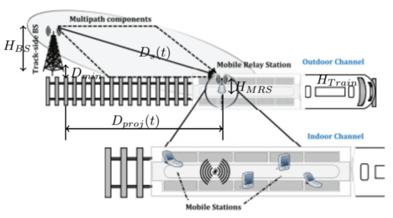
Figure 3.
Trigonometrical representation of open case environment for time-varying distance.
3. Statistical Properties of the Proposed 3D MIMO Wideband Non-Stationary HST Channel Model
The non-stationary correlation properties of two arbitrary CIRs of a MIMO HST channel can be deduced as,
where is the time-variant ST CF of the lth tap that can be expressed as
3.1. The Time-Variant ACF
The time-variant ACF can be obtained by imposing and in
By considering the Los component
where and . By considering the components for the first tap resulting from the sphere,
By considering the components for the lth tap resulting from the lth elliptical cylinder,
where and .
3.2. The Time-Variant CCF
By imposing in (3), we can obtain the time-variant space CCF between two arbitrary channel coefficients as
In the case of the Los component,
In the case of the SB components for the first tap resulting from the Rx circular cylinder,
In the case of the SB components for the lth tap resulting from the lth elliptical cylinder,
where and .
4. 3D Wideband Non-WSS Sum of Sinusoidal Simulation Model for MIMO HST Channel
Based on the proposed 3D theoretical GBSM described as from (1)–(3), the corresponding simulation model can be further developed by using finite numbers of scatterers and . This will be a complex tap coefficient for the link .
Method of Equal Volume and the Proposed Sum of Sinusoidal Simulation Model
The method of equal volume is used for the parameterization of the simulation model. This was used in [31,32] to determine the discrete angles of arrival and angles of departure for the simulation model. The objective of MEV is to determine the set of in such a manner that the volume of the VMF PDF in different ranges of are equal to each other with condition, i.e.,
where is the 3D VMF PDF introduced in (22).
5. Local Statistical Properties of the Proposed Sum of Sinusoidal Simulation Model
In this case, discrete time-varying parameters are applied to (3)–(12) to obtain the corresponding simulation model.
5.1. The Time-Variant ACF
The time-variant ACF can be derived by imposing and in (3)
By considering the Los component,
By considering the component for the first tap resulting from the sphere,
By considering the component for the tap resulting from the lth elliptical cylinder
5.2. The Time-Variant CCF
The time-variant space CCF between two arbitrary channel coefficients is obtained by imposing in (3) and thus,
By considering the Los component,
By considering the Los component,
By considering the component for the first tap resulting from the Rx sphere,
By considering the component for the ith tap resulting from the ith elliptical cylinder
5.3. The Time-Variant LCR
The LCR indicates how often the signal envelope crosses a given threshold of energy within a specified time per second. The pdf-based traditional method in [33] was used to derive the LCR for the derived model.
where is the function representing error, as , while . The parameters are defined as follows:
6. Analysis and Numerical Results
In this section, the generic model composed of the line of sight component (LOS), one sphere, and the multiple confocal elliptic cylinders was used to analyze the effect of train position and the two candidate mmWave carrier frequencies on the dynamic variances in the channel statistics for characterization. The impact of far distances and closer distances are investigated. The Rician factor and power-related factors are considered wheres parameters of , and are taken as in [34]. The antenna is assumed to be at the rooftop of the train.Some of the numerical parameters used are listed as in Table 2.
Table 2.
Numerical values used for the simulation model.
By using (23)–(26), Figure 4 depicts the time-variant ACF absolute values of the 3D theoretical model for the first and second tap at different time instants of s and s. The first tap has a higher correlation coefficient than the second tap due to the dominant LOS component. The autocorrelation function of the theoretical results and the simulation model exhibit a good approximation indicating the correctness of the proposed GBSM. Figure 5 shows the time variant CCF of the model for the first and second tap. The simulation model and the theoretical model are compared and the closesness is shown as in Figure 6. Therefore the model can be furthur applied for channel modelling. By using (27)–(33), Figure 7 depicts the absolute value of time-variant CCF of the simulation model for different mmWave carrier frequencies at different distances. The frequency at GHz has a higher correlation coefficient than that of GHz indicating a stronger line of sight at lower mmWave frequencies at far distances; therefore, the LOS of higher mmWave frequencies is affected by the distance between the transmitter and receiver. Figure 8 depicts the absolute value of time-variant CCF of the simulation model for different mmWave carrier frequencies at different closer distances. The mmWave carrier frequency at 60 GHz has a higher correlation than 28 GHz indicating a dominant LOS for higher mmWave frequencies in closer distances between and . Figure 9 shows the comparison between the simulation results from the proposed model and the measured results of stationary interval in [35]. This shows that the simulation results fit the measured results well with 9 ms for 80% and 19 ms for 20%. Figure 10 demonstrates that mmWave frequencies at 60 GHz have a longer stationary interval as the train is closer to the base station, therefore, by using the proposed model, we can capture non-stationarity channel statistics at mmWave frequencies. By imposing (34)–(35c), the LCR of the proposed model and the measured results from [36] are compared as shown in Figure 11. The results show that both the experimental and proposed model LCR reached a maximum value of 0.98 at a threshold value of 0 dB. The significant compatibility between the proposed generic model and the measurement reveals the usefulness of our HST generic channel model.
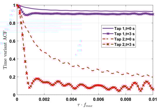
Figure 4.
The absolute values of the time-variant space ACF of different taps of the proposed HST channel model at different time instants.
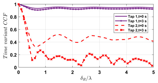
Figure 5.
The absolute values of the time-variant space CCF of different taps of the proposed HST channel model at different time instants.
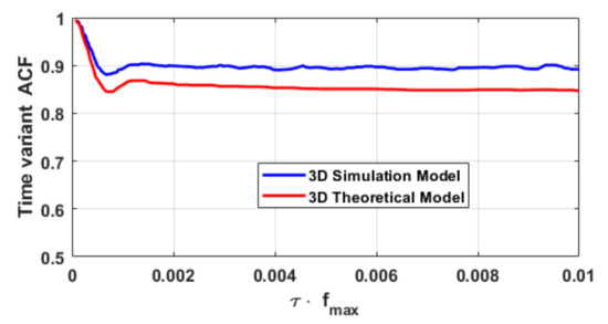
Figure 6.
The absolute values of the time-variant ACF of the 3D theoretical model, the 3D simulation model in open space scenario.
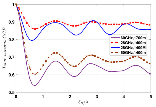
Figure 7.
The absolute values of the time-variant space CCF at GHz, GHz and far distances of m, m with km/h.
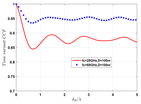
Figure 8.
The absolute values of the time-variant space CCF at GHz, GHz and close distances of m at km/h.
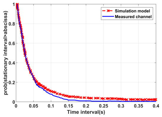
Figure 9.
The CCDF of the stationary interval simulated results and the measured results.
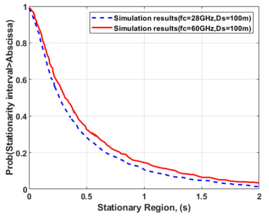
Figure 10.
Simulated CCDF of the stationary interval for different mmWave frequencies.
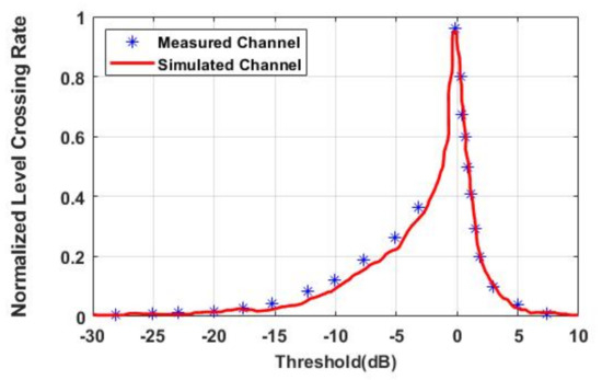
Figure 11.
The LCRs of the proposed HST channel model and the measured channel.
7. Conclusions
In this research paper, We have proposed a MIMO, 3D GBSM specifically one sphere and multiple focal elliptic cylinders to represent a non-stationary channel for the mmWave channel. The normalized channel statistics of the theoretical and simulation model have been derived. In addition, the proposed non-stationarity of the channel has been validated using measured data in terms of the stationary interval. The measurement of the stationarity interval has been further used to compare the two mmWave frequencies. We conclude that the distance and mmWave frequencies have a major impact on the local channel statistic properties. Consequently, the proposed model can represent non-stationarity as well as demonstrate the impact of mmWave frequencies on channel statistics. In addition, Since the MIMO channel has been modeled in 3D, the antenna array configuration could be extended to massive MIMO in a different plane, such as cylindrical or spherical, which makes the signal radiation more practical.
Author Contributions
Conceptualization, E.A. and Y.W.M.; methodology, E.A.; software, E.A.; validation, Y.W.M.; formal analysis, Y.W.M.; investigation, E.A.; resources, E.A.; writing—original draft preparation, E.A.; writing—review and editing, Y.W.M. and E.A.; visualization, Y.W.M.; supervision, Y.W.M. All authors have read and agreed to the published version of the manuscript.
Funding
This research received no external funding.
Conflicts of Interest
The authors declare no conflict of interest.
References
- Ai, B.; Cheng, X.; Kurner, T.; Zhong, Z.D.; Guan, K.; He, R.S.; Xiong, L.; Matolak, D.W.; Michelson, D.G.; Briso-Rodriguez, C. Challenges toward wireless communications for high-speed railway. IEEE Trans. Intell. Transp. Syst. 2014, 15, 2143–2158. [Google Scholar] [CrossRef]
- Zhao, X.; Li, S.; Wang, Q.; Wang, M.; Sun, S.; Hong, W. Channel measurements, modeling, simulation and validation at 32 GHz in outdoor microcells for 5g radio systems. IEEE Access 2017, 5, 1062–1072. [Google Scholar] [CrossRef]
- Zhao, X.; Liang, X.; Li, S.; Ai, B. Two-cylinder and multi-ring GBSM for realizing and modeling of vehicle-to-vehicle wideband MIMO. channels. IEEE Trans. Intell. Transp. Syst. 2016, 17, 2787–2799. [Google Scholar] [CrossRef]
- Liu, Y.; Wang, C.-X.; Huang, J. Recent developments and future challenges in channel measurements and models for 5G and beyond high-speed train communication systems. IEEE Commun. Mag. 2019, 57, 50–56. [Google Scholar] [CrossRef]
- Pavia, J.P.; Velez, V.; Souto, N.; Ribeiro, M.; Sebastião, P.; Correia, A. System-Level Assessment of Low Complexity Hybrid Precoding Designs for Massive MIMO Downlink Transmissions in Beyond 5G Networks. Appl. Sci. 2022, 12, 2812. [Google Scholar] [CrossRef]
- Wang, C.-X.; Bian, J.; Sun, J.; Zhang, W.; Zhang, M. A survey of 5G channel measurements and models. IEEE Commun. Surv. Tutor. 2018, 20, 3142–3168. [Google Scholar] [CrossRef]
- Mao, K.; Zhu, Q.; Song, M.; Hua, B.; Zhong, W.; Ye, X. A Geometry-Based Beamforming Channel Model for UAV mmWave Communications. Sensors 2020, 20, 6957. [Google Scholar] [CrossRef] [PubMed]
- Xiao, Y.; Qiu, G.; Wang, Y. A Fast Hybrid Beamforming Scheme for High-Speed Railway Communications. Electronics 2019, 8, 998. [Google Scholar] [CrossRef] [Green Version]
- Riviello, D.G.; Di Stasio, F.; Tuninato, R. Performance Analysis of Multi-User MIMO Schemes under Realistic 3GPP 3-D Channel Model for 5G mmWave Cellular Networks. Electronics 2022, 11, 330. [Google Scholar] [CrossRef]
- Aredo, S.C.; Negash, Y.; Marye, Y.W.; Kassa, H.B.; Kornegay, K.T.; Diba, F.D. Hardware Efficient Massive MIMO Systems with Optimal Antenna Selection. Sensors 2022, 22, 1743. [Google Scholar] [CrossRef]
- He, D.; Ai, B.; Guan, K.; Wang, L.; Zhong, Z.; Krner, T. The design and applications of a high-performance ray-tracing simulation platform for 5G and beyond wireless communications: A tutorial. IEEE Commun. Surv. Tutor. 2018, 21, 10–27. [Google Scholar] [CrossRef]
- Guan, K.; Li, G.; Kürner, T.; Molisch, A.F.; Peng, B.; He, R.; Hui, B.; Kim, J.; Zhong, Z. On millimeter-wave and THz mobile radio channel for smart rail mobility. IEEE Trans. Veh. Technol. 2017, 66, 5658–5674. [Google Scholar] [CrossRef]
- Feng, L. A stochastic confocal ellipsoid channel model for high-speed railway MIMO communication systems. Phys. Commun. 2022, 52, 101616. [Google Scholar] [CrossRef]
- Azpilicueta, L.; Lopez-Iturri, P.; Zuñiga-Mejia, J.; Celaya-Echarri, M.; Rodríguez-Corbo, F.A.; Vargas-Rosales, C.; Aguirre, E.; Michelson, D.G.; Falcone, F. Fifth-Generation (5G) mmWave Spatial Channel Characterization for Urban Environments’ System Analysis. Sensors 2020, 20, 5360. [Google Scholar] [CrossRef]
- Ghazal, A.; Wang, C.-X.; Haas, H.; Beach, M.; Mesleh, R.; Yuan, D.; Ge, X.; Chahine, M.H. A non-stationary geometry-based stochastic model for MIMO high-speed train channels. IEEE Commun. Surv. Tutor. 2019, 21, 10–27. [Google Scholar]
- Hrovat, A.; Bregar, K.; Javornik, T. Measurement-based ultra-wideband channel model for mobile communications in tunnels. In Proceedings of the 12th European Conference on Antennas and Propagation (EuCAP 2018), London, UK, 9–13 April 2018. [Google Scholar]
- He, R.; Ai, B.; Stuber, G.L.; Wang, G.; Zhong, Z. A cluster based geometrical model for millimeter wave mobile-to-mobile channels. In Proceedings of the 2017 IEEE/CIC International Conference on Communications in China (ICCC), Qingdao, China, 22–24 October 2017. [Google Scholar]
- Lu, J.; Zhu, G.; Ai, B. Radio propagation measurements and modeling in railway viaduct area. In Proceedings of the 2010 International Conference on Computational Intelligence and Software Engineering, Wuhan, China, 10–12 December 2010. [Google Scholar]
- Lu, J.; Zhu, G.; Briso-Rodriguez, C. Fading characteristics in the railway terrain cuttings. In Proceedings of the 2011 IEEE 73rd Vehicular Technology Conference (VTC Spring), Budapest, Hungary, 15–18 May 2011. [Google Scholar]
- Luan, F.; Zhang, Y.; Xiao, L.; Zhou, C.; Zhou, S. Fading characteristics of the wireless channel on a high-speed railway in a hilly terrain scenario. Int. J. Antennas Propag. 2013, 2013, 378407. [Google Scholar] [CrossRef] [Green Version]
- Rodríguez-Piñeiro, J.; Suárez-Casal, P.; Lerch, M.; Caban, S.; Garcia-Naya, J.A.; Castedo, L.; Rupp, M. LTE downlink performance in high-speed trains. In Proceedings of the 2015 IEEE 81st Vehicular Technology Conference (VTC Spring), Glasgow, Scotland, 11–14 May 2015. [Google Scholar]
- Sun, R.; Tao, C.; Liu, L.; Tan, Z.; Zhang, L.; Zhou, T. Nonisotropic scattering characteristic in an alternant tree-blocked viaduct scenario on a high-speed railway at 2.35 GHz. Int. J. Antennas Propag. 2014, 2014, 642894. [Google Scholar] [CrossRef] [Green Version]
- UIC—International Union of Railways. UIC—International Union of Railways—The Worldwide Railway Organization. 2016. Available online: http://www.uic.org/spip.php?rubrique851 (accessed on 10 May 2022).
- Wang, C.X.; Hong, X.; Ge, X.; Cheng, X.; Zhang, G.; Thompson, J. Cooperative MIMO channel models: A survey. IEEE Commun. Mag. 2010, 48, 80–87. [Google Scholar] [CrossRef]
- Samimi, M.K.; MacCartney, G.R.; Sun, S.; Rappaport, T.S. 28 GHz millimeter-wave ultrawideband small-scale fading models in wireless channels. In Proceedings of the 2016 IEEE 83rd Vehicular Technology Conference (VTC Spring), Nanjing, China, 15–18 May 2016. [Google Scholar]
- Kim, W. Experimental Demonstration of MmWave Vehicle-to-Vehicle Communications Using IEEE 802.11ad. Sensors 2019, 19, 2057. [Google Scholar] [CrossRef] [Green Version]
- Guan, K.; Lin, X.; He, D.; Ai, B.; Zhong, Z.; Zhao, Z.; Miao, D.; Guan, H.; Kürner, T. Scenario modules and ray-tracing simulations of a millimeter-wave and terahertz channels for smart rail mobility. In Proceedings of the 2017 11th European Conference on Antennas and Propagation (EUCAP), Paris, France, 19–24 March 2017; pp. 1445–1449. [Google Scholar]
- Lopez, C.F.; Wang, C.X. Novel 3D non-stationary wideband models for massive MIMO channels. IEEE Trans. Wirel. Commun. 2018, 17, 2905. [Google Scholar] [CrossRef] [Green Version]
- Yuan, Y.; Wang, C.X.; Cheng, X.; Ai, B.; Laurenson, D.I. Novel 3D geometry-based stochastic models for non-isotropic MIMO vehicle-to-vehicle channels. IEEE Trans. Wirel. Commun. 2013, 13, 298–309. [Google Scholar] [CrossRef] [Green Version]
- Cai, X.; Giannakis, G.B. A two-dimensional channel simulation model for shadowing processes. IEEE Trans. Veh. Technol. 2003, 52, 1558–1567. [Google Scholar]
- Yuan, Y.; Wang, C.X.; He, Y.; Alwakeel, M.M. 3D wideband non-stationary geometry-based stochastic models for non-isotropic MIMO vehicle-to-vehicle channels. IEEE Trans. Wirel. Commun. 2015, 14, 6883–6895. [Google Scholar] [CrossRef]
- Zhao, M.; Wu, M.; Sun, Y.; Yu, D.; Di, S.; Zhou, P.; Zeng, X.; Ge, S. Analysis and modeling for a train-ground wireless wideband channel of LTE on a high-speed railway. In Proceedings of the 2013 IEEE 77th Vehicular Technology Conference (VTC Spring), Dresden, Germany, 2–5 June 2013. [Google Scholar]
- Youssef, N.; Wang, C.-X.; Patzold, M. A study on the second-order statistics of Nakagami-Hoyt mobile fading channels. IEEE Trans. Veh. Technol. 2005, 54, 1259–1265. [Google Scholar] [CrossRef]
- TS36.104; Base Station (BS) Radio Transmission and Reception (Release 11). Generation Partnership Project. Technical Specification Group Radio Access Network. Evolved Universal Terrestrial Radio Access (E-UTRA): Sophia-Antipolis, France, 2013.
- Chen, B.; Zhong, Z.; Ai, B. Stationarity intervals of a time-variant channel in high-speed railway scenario. J. China Commun. 2012, 9, 64–70. [Google Scholar]
- Yue, G.; Yu, D.; Cheng, L.; Lv, Q.; Luo, Z.; Li, Q.; Luo, J.; He, X. Millimeter-wave system for high-speed train communications between train and trackside: System design and channel measurements. IEEE Trans. Veh. Technol. 2019, 68, 11746–11761. [Google Scholar] [CrossRef]
Publisher’s Note: MDPI stays neutral with regard to jurisdictional claims in published maps and institutional affiliations. |
© 2022 by the authors. Licensee MDPI, Basel, Switzerland. This article is an open access article distributed under the terms and conditions of the Creative Commons Attribution (CC BY) license (https://creativecommons.org/licenses/by/4.0/).