High-Resolution Delay Spread of Wide-Band Wireless Link in Long Tunnels—Theory and Experimental Verification

Abstract

The need for wireless communication appears everywhere, and with as few interruptions as possible. An extensive and in-depth study has been conducted on the limitations of wireless communication in pedestrian tunnels. Using an analytical mathematical ray tracing model, and performing tunnel measurements, with an autonomous measuring setup, the model was validated. An extraordinary wide band was used for the experiments, which also featured optical systems to ensure accurate results. Since the tunnel is narrow, the differences between the different paths are small, and in order to distinguish them a resolution of 0.2 ns was used. The RMS delay spread, ${\sigma }_{\tau }$, decreases throughout the tunnel, and at no point exceeds 1 ns.

1. Introduction

Wireless communication has never been more popular [1]. The 5G rates for data and availability are today’s standard, with 6G right around the corner [2]. Wireless communication is crucial for performing many of our daily tasks. The reliability of the communication link is a critical issue and in some cases there is no room for error.

One of the primary limitations of wireless communication in tunnels is constructive and destructive interference caused by reflections from walls [3]. However, the influence of each of the components that produce this phenomenon is insufficiently clear. These components may include: the transmission frequency, length and height of the tunnel, the location and polarization of the antennas, the type of tunnel and the roughness of its walls.

One of the main parameters with which the performance of a communication link is measured is root mean square (RMS) delay spread, ${\sigma }_{\tau }$. RMS delay spread describes the duration it takes for all the reflections from a broadcast at a given moment to reach the receiver; in other words, it provides us with the data rate that can be transmitted with the link.

Table 1. RMS Delay Spread typical values.

Environment	Center Frequency (MHz)	Bandwidth (MHz)	${\mathit{\sigma }}_{\mathit{\tau }}$ (ns)
Urban—New York City [4]	910	10	1300
Suburban [4]	910	10	200–310
Indoor—Office Building [5]	1500	500	25
Underground Mine
Channel [6]	3500	3000	11.8
Uneven Underground
Mine Channel [7]	2400	200	9.92

shows typical RMS delay spread times in different environments.

A common approach is to perform an experiment on a specific site without basing the research on any calculations and theoretical model [7,8,9,10,11,12,13,14]. In this form of work, one can learn about a single and specific case, without the ability to generalize to different cases.

Similarly, the opposite case also exists [15,16]: Performing only simulated results, without any experimental verification. This may lead to a situation where a variety of variables are not taken into account while performing the sterile calculations in the simulation, which will lead to invalid results. Therefore, the simulation should be validated with an experiment.

In many studies the bandwidth that was used was very limited [7,12,13,17,18]. This is contrary to the desire to get as high quality results as possible. However, in order to obtain results that accurately reflect the limitations of the tunnel, it is necessary to perform high-resolution measurements. Thus, in order to obtain a higher resolution for measurements in time domain it is necessary to increase the bandwidth in the frequency domain when making the measurements.

Other studies have based their research on experiments with very low measuring resolution [19]: That is, a very limited number of points along the tunnel. Alternatively, the whole length of their experiment was very short [18,20]. In such a situation, it is not possible to get an accurate snapshot, as the signal behavior in the tunnel is not linear or predictable and there are frequent changes along the tunnel.

A common issue in wireless communication experiments is the additional phase added to the results by the measuring equipment. To avoid this phenomenon, fiber optics can be used, since they do not change the phase. Some studies on this subject were aided by fiber optics [19,21], but no in-depth campaign was carried out.

Although similar studies have been previously conducted by other authors, no in-depth and sufficiently accurate investigation has been conducted. In this study, a comprehensive study is conducted on the limitations of wireless communication in tunnels. A frequency range of 1–6 GHz was used to provide an extra large bandwidth of 5 GHz. The large bandwidth in the frequency domain gives us a high resolution in the time domain of 0.2 ns. A long in-depth measurement campaign was carried out in a long pedestrian tunnel. The experimental results were compared to a mathematical model, validating the mathematical model.

2. The Delay Spread Theory in Tunnels and Long Corridors

Electromagnetic wave propagation inside tunnels suffers from multi-path interference, which distorts the received signal due to constructive and destructive waves arriving simultaneously at the receiver. The propagation depends on different parameters such as: Construction materials, antenna polarization, transmitter and receiver location in the cross-sectional area, the separation between the transmitter and receiver, and so on. It is described using (1): [22,23]

$${\tilde{H}}_{norm}\left(jf\right)=\frac{{\tilde{E}}_r\left(Tunnel\right)}{{\tilde{E}}_r\left(LOS\right)}=\sum _{m=-\infty }^{+\infty }\sum _{n=-\infty }^{+\infty }\underset{{\tilde{A}}_{mn}}{\underbrace{\frac{R_0}{R(m,n)}·{\Gamma }_{\alpha }^{\left|m\right|}·{\Gamma }_{\beta }^{\left|n\right|}·\frac{G(\theta ,\varphi )}{G_{LOS}}}}·e^{-j2\pi f\Delta \tau (m,n)}$$

(1)

${\tilde{H}}_{norm}\left(jf\right)$ is normalized to the LOS ray for convenience.

$R_0=R(0,0)$ is the line of sight (LOS) ray length and $R(m,n)$ is the length of the path that the n’th and m’th order of reflected ray has traveled, as described in (2):

$$R(m,n)=\sqrt{{[x_t\left(m\right)-x_r]}^2+{[y_t\left(n\right)-y_r]}^2+z^2}$$

(2)

The image coordinates of the transmitter are defined in (3):

$$x_t\left(m\right)=2ma+{(-1)}^m·x_t\mathrm{and}{x}_t\left(m\right)=2ma+{(-1)}^m·x_t$$

(3)

when a represents half of the width of the tunnel and b represents half of the tunnel’s height. The reflection coefficient, $\Gamma$, is calculated using Fresnel’s equations. Since one reflection coefficient will be transverse electric (TE) and the other transverse magnetic (TM) depending on the polarization of the antenna [23,24], they were marked ${\Gamma }_{\alpha }^{\left|m\right|}$ and ${\Gamma }_{\beta }^{\left|n\right|}$. m represents the number of reflections in the horizontal dimension, and n is the same but in the vertical dimension. f is the frequency of the wave. For a directive link, $G(\theta ,\varphi )$ is the geometrical mean gain of both the transmitter and receiver antennas, $G(\theta ,\varphi )=\sqrt{G_t(\theta ,\varphi )·G_r(\theta ,\varphi )}$, and $G_{LOS}$ is the gain of the antenna for the LOS ray.

For simplicity, we define $A_{mn}$ as the following (4):

$${\tilde{A}}_{mn}=\frac{R_0}{R(m,n)}·{\Gamma }_{\alpha }^{\left|m\right|}·{\Gamma }_{\beta }^{\left|n\right|}·\frac{G(\theta ,\varphi )}{G_{LOS}}$$

(4)

The propagation time for the LOS ray from the transmitter to the receiver is defined in (5):

$${\tau }_0=\frac{R_0}{c}$$

(5)

The propagation time delay of each of the other rays is defined as follows (6):

$$\tau (m,n)=\frac{R(m,n)}{c}={\tau }_0+\Delta \tau (m,n)$$

(6)

where $\Delta t(m,n)$ is the additional time that the $(m,n)$ ray travels more then the LOS ray travels.

Assuming the antenna’s gain is not dependent on the frequency, the impulse response is:

$$h\left(t\right)={\mathcal{F}}^{-1}\left\{{\tilde{H}}_{norm}\left(jf\right)\right\}=Re\{{\int }_0^{\infty }{\tilde{H}}_{norm}\left(jf\right)·e^{+j2\pi ft}df\}=Re\left\{{\displaystyle \sum _{m=-\infty }^{+\infty }}{\displaystyle \sum _{n=-\infty }^{+\infty }}{\tilde{A}}_{mn}·\delta [t-\Delta \tau (m,n)]\right\}$$

(7)

The Power Delay Profile (PDP) of the channel, $P_h\left(\tau \right)$, describes how much power (from a transmitted delta pulse with unit energy) is transferred to the receiver with a delay of $\tau$ from the moment of transmission.

The Power Delay Profile is acquired from the normalized complex impulse response as described in (7) and defined as follows [25]:

$$P_h\left(\tau \right)=\frac{{\left|h\left(\tau \right)\right|}^2}{{\parallel h\left(\tau \right)\parallel }^2}$$

(8)

where the norm of $h\left(\tau \right)$ is defined by (9):

$${\parallel h\left(\tau \right)\parallel }^2={\int }_{-\infty }^{+\infty }{\left|h\left(\tau \right)\right|}^{2}d\tau ={\int }_0^{\infty }|{\tilde{H}}_{norm}{\left(jf\right)|}^{2}df=\sum _{m=-\infty }^{+\infty }\sum _{n=-\infty }^{+\infty }{\left|{\tilde{A}}_{mn}\right|}^2$$

(9)

From the last definition, it follows that:

$${\int }_{-\infty }^{+\infty }{P}_h\left(\tau \right)d\tau =1$$

(10)

The PDP is the probability density function (PDF) of the delay $\tau$ of an impulse, with dimensions of [$\frac{1}{sec}$].

The average (mean) delay of all the paths is defined as $\overline{\tau }$ [18]:

$$\overline{\tau }=\langle \tau \rangle ={\int }_{-\infty }^{+\infty }\tau ·P_h\left(\tau \right)d\tau =\frac{{\displaystyle \sum _{m=-\infty }^{+\infty }}{\displaystyle \sum _{n=-\infty }^{+\infty }}{\tau }_{mn}·{\left|{\tilde{A}}_{mn}\right|}^2}{{\parallel h\left(\tau \right)\parallel }^2}=\frac{{\displaystyle \sum _{m=-\infty }^{+\infty }}{\displaystyle \sum _{n=-\infty }^{+\infty }}{\tau }_{mn}·{\left|{\tilde{A}}_{mn}\right|}^2}{\underset{{\parallel h\left(\tau \right)\parallel }^2}{\underbrace{{\displaystyle \sum _{m=-\infty }^{+\infty }}{\displaystyle \sum _{n=-\infty }^{+\infty }}{\left|{\tilde{A}}_{mn}\right|}^2}}}$$

(11)

RMS delay spread, shown as ${\sigma }_{\tau }$ in (12), is the standard deviation. In our case, it is an appraisal of the smallest time required between transmission of symbols, in a way that will prevent inter-symbol interference (ISI) [26].

$${\sigma }_{\tau }=\sqrt{\langle {\tau }^2\rangle -{\left(\overline{\tau }\right)}^2}$$

(12)

where

$$\langle {\tau }^2\rangle ={\int }_{-\infty }^{+\infty }{\tau }^2·P_h\left(\tau \right)d\tau =\frac{{\displaystyle \sum _{m=-\infty }^{+\infty }}{\displaystyle \sum _{n=-\infty }^{+\infty }}{\tau }_{mn}^2·{\left|{\tilde{A}}_{mn}\right|}^2}{\underset{{\parallel h\left(\tau \right)\parallel }^2}{\underbrace{{\displaystyle \sum _{m=-\infty }^{+\infty }}{\displaystyle \sum _{n=-\infty }^{+\infty }}{\left|{\tilde{A}}_{mn}\right|}^2}}}$$

(13)

Substituting $\overline{\tau }$ and $\langle {\tau }^2\rangle$ into (12), the expression for ${\sigma }_{\tau }$ results in (14):

$${\sigma }_{\tau }=\sqrt{\langle {\tau }^2\rangle -{\left(\overline{\tau }\right)}^2}=\sqrt{\frac{{\displaystyle \sum _{m=-\infty }^{+\infty }}{\displaystyle \sum _{n=-\infty }^{+\infty }}{\tau }_{mn}^2·{\left|{\tilde{A}}_{mn}\right|}^2}{\underset{{\parallel h\left(\tau \right)\parallel }^2}{\underbrace{{\displaystyle \sum _{m=-\infty }^{+\infty }}{\displaystyle \sum _{n=-\infty }^{+\infty }}{\left|{\tilde{A}}_{mn}\right|}^2}}}-{\left[\frac{{\displaystyle \sum _{m=-\infty }^{+\infty }}{\displaystyle \sum _{n=-\infty }^{+\infty }}{\tau }_{mn}·{\left|{\tilde{A}}_{mn}\right|}^2}{\underset{{\parallel h\left(\tau \right)\parallel }^2}{\underbrace{{\displaystyle \sum _{m=-\infty }^{+\infty }}{\displaystyle \sum _{n=-\infty }^{+\infty }}{\left|{\tilde{A}}_{mn}\right|}^2}}}\right]}^2}$$

(14)

Since we have described the propagation of the signal in space as rays sent in all directions, it is necessary to specify which rays we will refer to. On the one hand, the number of rays tends to infinity, and on the other hand in terms of mathematical model calculations it is certainly not possible to reach such accuracy.

The number of relevant rays depends very much on the parameters of the communication (wavelength, tunnel size, distance). In an earlier study we conducted [23], we examined the error as a function of the number of rays. We have seen that there is certainly some improvement with the results compared to the experiment as more rays are considered. However, even with a small number of rays the results are satisfactory. To avoid mistakes and inaccuracies, in this study, we took into consideration rays that bounced off the walls up to 30 times and off the ceilings or floor up to 30 times as well, before arriving at the receiver, which is above and beyond any required level of accuracy.

As described, the reflected rays propagate along the tunnel at different times, thus not reaching the receiver simultaneously. In order to paint a clearer picture of this phenomenon, we will demonstrate this by using an example of a tunnel’s impulse response from the model. The model was run in a case that represents the dimensions of the tunnel that will be used in the experiment, as detailed in

Table 2. Model example parameters.

Parameters	Value
Frequency	1.5 GHz
Power transmitted	20 dBm
a (half of the tunnels width)	0.5 m
b (half of the tunnels height)	0.925 m
Length	20 m
Material	concrete

. The signal was transmitted at the beginning of the tunnel and recorded at the end of the tunnel.

The plot, as shown in Figure 1, visualizes each ray arriving at different times at the receiver. The first ray to arrive represents the LOS ray which has the shortest flight time, and gradually thereafter all the rest of the rays which did not have a direct path will appear. The Y axis represents normalized values of the received power in relation to the transmitted power.

To present normalized time values of the received arrays in relation to the LOS array, we define (15):

$$t_{normalized}=\frac{L_{m,n}-d}{d}=\frac{\Delta t}{t_r}$$

(15)

where $L_{m,n}$ is the distance that the $m,n$ ray travels, d is the length between the transmitter and receiver which the LOS ray travels, in this case d = 20 m, $\Delta t$ is the additional time the $m,n$ ray travels, and $t_r$ is the LOS the ray travels.

In the following sections, the analytically calculated and experimental outcome of, inter alia, $S_{21}$, time domain results and RMS delay spread in a long pedestrian tunnel are presented.

3. Experimental Setup

The measurements were performed in the frequency domain, using a Keysight Streamline USB Vector Network Analyzer (VNA) model number P9371A, as can be seen in Figure 2. A VNA measures the scattering parameters, which describe the relationship between the different ports. A network analyzer is especially useful when the effect of the network in terms of amplitude and phase need to be described. During the experiment, the complex $S_{21}$ parameter was measured, which represents the difference in amplitude and phase between port 1, the transmitter (Tx), and port 2, the receiver (Rx).

The VNA is a portable device, allowing for use in the tunnel in order to receive results as accurate as possible. The VNA parameters are detailed in

Table 3. Vector network analyzer parameters.

Parameters	Value
Manufacturer	Keysight
Model	P9371A
Frequency range	300 kHz to 6.5 GHz

.

The transmitting antenna was connected to Port 1, which was placed at the entrance to the tunnel without movement throughout the experiment. In contrast, the receiving antenna, which was connected to Port 2, was moved along the tunnel prior to each measurement.

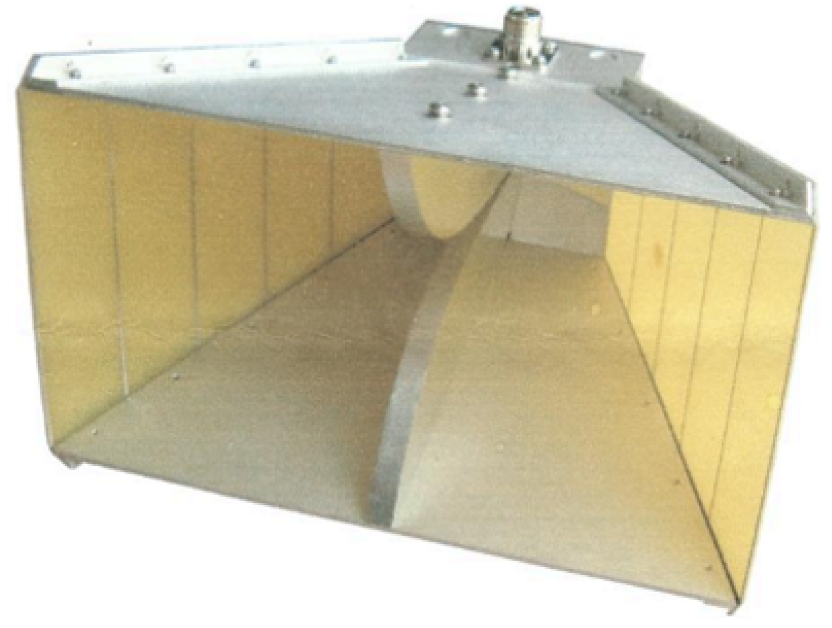
A broadband horn antenna as shown in Figure 3 was used at both ports, as detailed in

Table 4. Wide-band Horn Antenna Parameters.

Parameters	Value
Manufacturer	Chendgu A-INFO
Model	JXTXLB-10180
Frequency range	1–18 GHz
Gain	11 dBi Typical
Polarization	Linear
VSWR	2.0:1 Typical
H-Plane 3dB Beamwidth	37–71
E-Plane 3dB Beamwidth	39.7–70

. This was done so that as much power as possible will be in the direction of the transmission, in order to intensify the reflections from the tunnel walls.

Although the antenna supports a wide spectrum of frequencies, the antenna gain varies according to the frequency. The gain and antenna factor were measured in an antenna test range, the results of which can be seen in

Table 5. Gain and antenna factor.

Frequency	Antenna Factor $\left({\mathbf{dBm}}^{\mathbf{-}\mathbf{1}}\right)$	Gain $\left(\mathbf{dBi}\right)$
1	23.63	6.63
1.5	24.18	9.6
2	26.03	10.25
3	29.8	9.98
4	31.60	10.7
6	33.97	11.85

.

In order to eliminate the uneven frequency response of the antennas, a calibration operation was activated in the VNA prior to the experiment. Thus, the VNA takes into account the frequency response of the antenna in the calculation of the S21 so that the S21 only expresses the propagation.

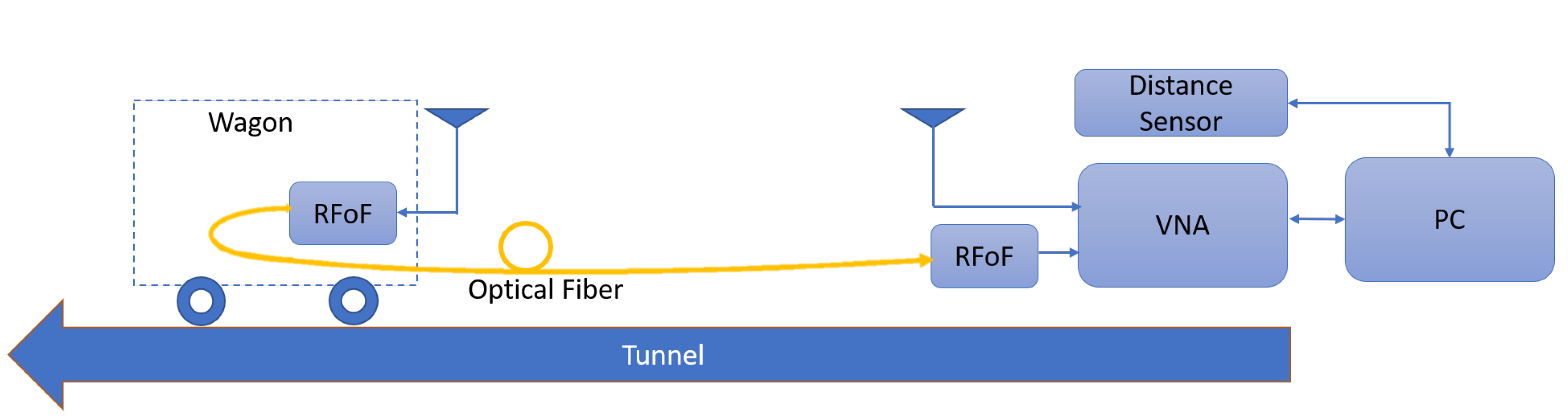
To ensure that the measurement process performs smoothly and gives us the ability to sample the effect of the tunnel many times along the tunnel, an autonomous measuring setup was designed as shown in Figure 4 which parameters are detailed in

Table 6. Measurement parameters.

Frequency range	1–6 GHz
Number of samples	11130
Transmission power	20 dBm
Receiver IF bandwidth	1 kHz
Frequency resolution	0.45 MHz
Time resolution	0.2 ns
Maximum excess delay	2.2 µsec

.

In order to perform autonomous measuring, the VNA was controlled by a PC running Standard Commands for Programmable Instruments (SCPI) coding sent from the MATLAB environment. With the help of this, there was full control over the timing of the measurement and synchronization with the distance data. Additionally, this enabled the results to be stored on the PC for later processing.

In order to accurately measure the distance between the antennas, a Laser Distance Measuring Sensor was used. The distance sensor was connected to the PC via RS232 serial data connection. These serial commands were likewise sent from the MATLAB environment. The laser was placed at the entrance of the tunnel, next to the transmitting antenna. Simultaneously, with each measurement that was performed by the network, a measurement was performed by the distance sensor. In this way, coordinated measurements were obtained.

With the intention of measuring the S21, it is necessary that the receiving antenna will likewise be connected to the network analyzer. Since in the experiment the receiving antenna is on the other side of the tunnel, this phenomenon was accomplished using an optical fiber. The RF signal obtained in the receiving antenna was transformed to an optical signal in order to be transmitted on an optical fiber. The signal traveled through the optical fiber along the tunnel back towards the VNA, which is then converted back to RF before connecting to the VNA. Since the measurements were performed along the tunnel, the separation between the antennas increased with every measurement. With a regular coax cable, every movement causes a change in the phase, and by using an optical fiber this phenomenon is avoided. The additional delay caused by the RF optic device, and the time it took the signal to travel back along the optical fiber, were taken into account and did not affect the measurement results.

The RF Optic device as shown in Figure 5 supports up to 6 GHz with a nominal link gain of 7 dB. The optical signal is transmitted with a 1310 nm wavelength [27]. The device has the ability to increase the signal transmitted via the optical fiber with an LNA. In the experiments, the LNA was not used, since this brought the signal to saturation.

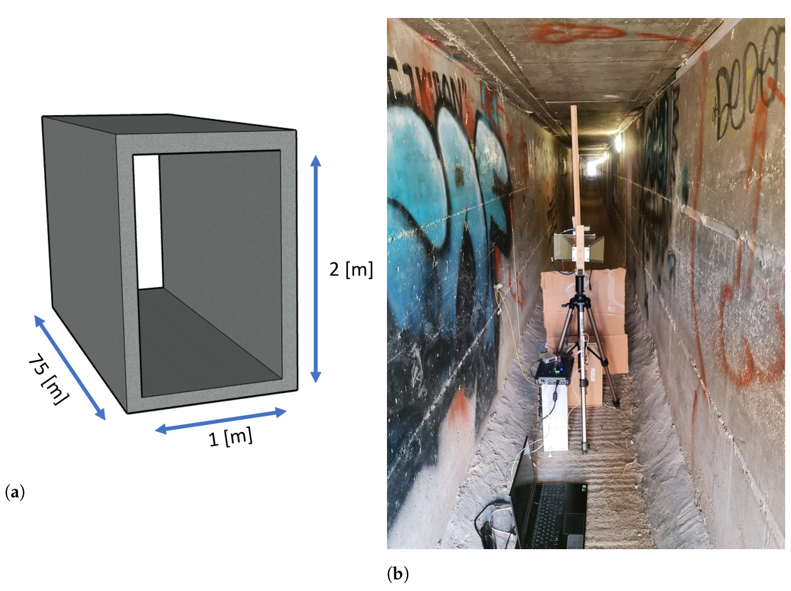
The experiments were performed in a pedestrian tunnel under a highway. The tunnel is long and straight. The walls are mostly smooth, but there was a certain roughness in between the smooth plates of the concrete. The dimensions of the underpass are: $Height=2b$ = 1 m, $Width=2a$ = 1.85 m and $Length$ = 75 m, as shown in Figure 6a.

The measurements were carried out along the tunnel, while the transmitting and receiving antennas were placed in the middle of the cross-sectional area of the tunnel. The tunnel was empty throughout the whole measurement process, and therefore there was no interference between the transmitter and receiver.

The transmitter antenna was connected to an antenna stand. The receiving antenna was attached to a pole which was part of the wooden wagon. To give the laser a surface to reflect off of, cardboard was attached to the front of the cart. All components of the experiment were unable to wobble, besides the optical fiber which was loose, enabling it to extend along the tunnel. The experiment setup at the experiment site can be seen in Figure 6b.

4. Tunnel Propagation Characterization via S-Parameters

As a result of the measurements that were performed in the tunnel, the complex $S_{21}$ parameter was obtained along the tunnel. Since the results represent the characteristics of a single tunnel, the results were compared to the simulation results in order to confirm the correctness of the model. In this way, simulation results can be obtained in other unmeasured cases as well, which supplies us with a broader understanding of electromagnetic wave propagation in tunnels.

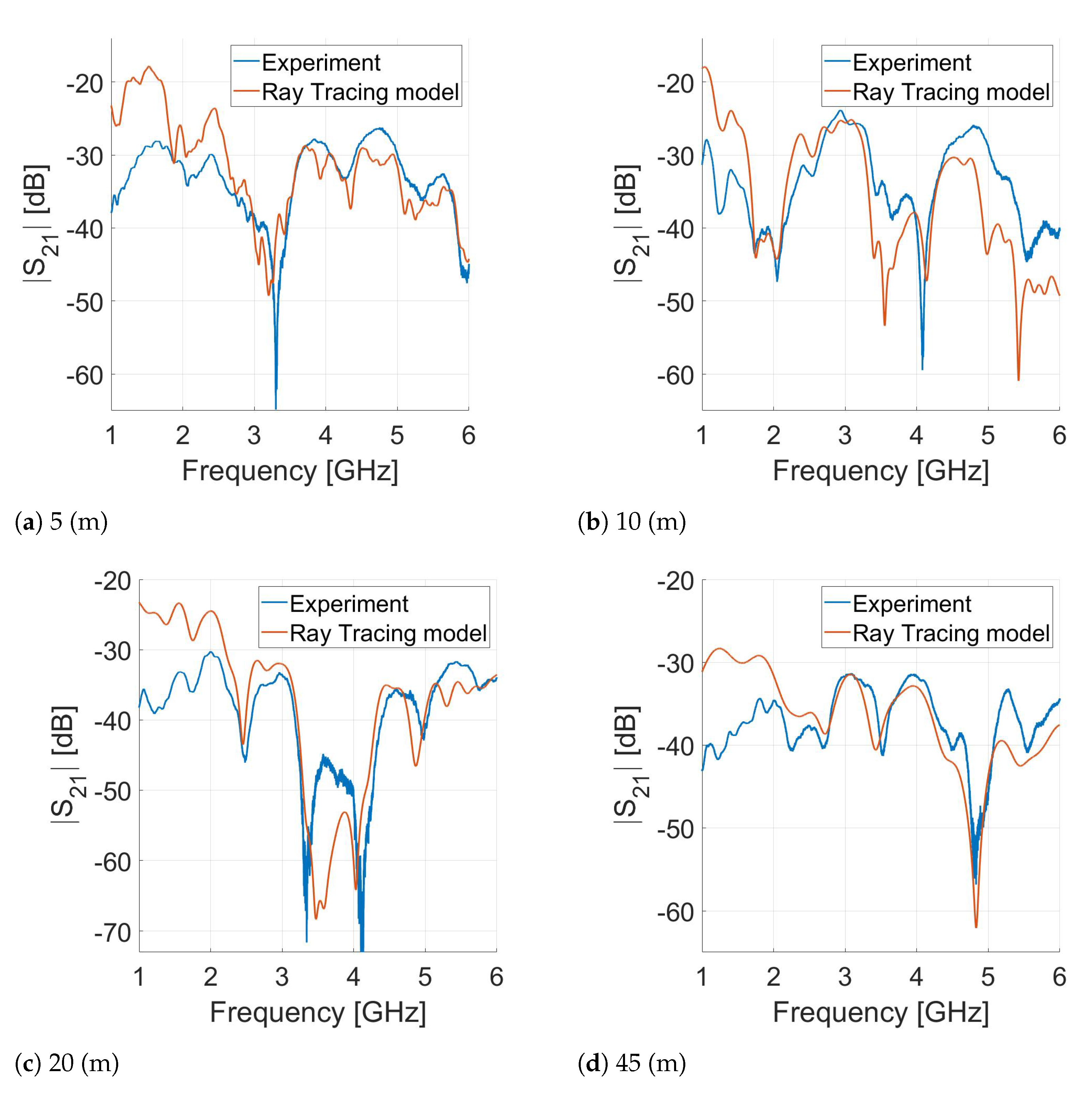
The first result is essentially one of the basic parameters measured by the network analyzer, the power received versus frequency. The received power was plotted in Figure 7, for 5, 10, 20 and 45 m of distance between the transmitter and receiver. These distances constitute a representative sample along the tunnel. The results from the experiment were plotted with the results from the simulation, so a comparison can be performed between them.

The received power visualizes the selective fading of the frequency that is caused by the tunnel. As is clearly noticeable, the power has peaks and dips in various frequencies, as a consequence of constructive and destructive interference. Hence, the powers received at distinctive frequencies differ from each other.

The experiment results were plotted with the simulation results, so that a comparison can be made between them. The comparison shows a high similarity between the experiment and simulation. Among the general results obtained, there is a good match, but especially in the location of the peaks and dips there is a precise match. The precise match in the location of the peaks and dips is of high importance since they have the greatest effect on the communication performance, more than the power obtained at any specific location.

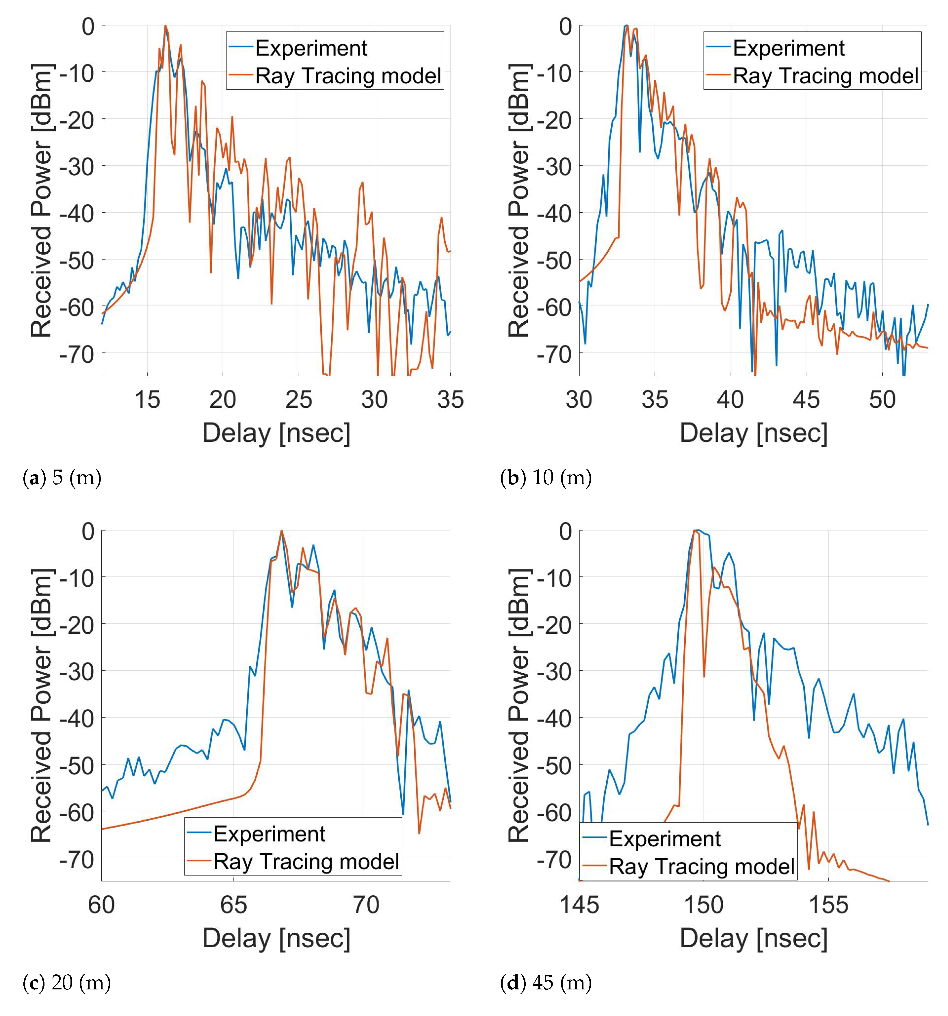
5. Power Delay Profile Measurements

The IFFT function was applied to the frequency domain results in the time domain. By doing so we obtained the Power Delay Profile (PDP) as described in (8). The PDP was normalized and plotted in Figure 8, for 5, 10, 20 and 45 m of distance between the transmitter and receiver.

This visualization of the experiment and simulation data can offer a clearer understanding of the multi-path components that reflect off the walls on their way to the receiver. The multi-path components can challenge the use of high data rates [28,29]. The PDP plot demonstrates the different rays received at the receiver.

For example, in the case of a 5 m gap between the transmitter and the receiver, the LOS ray reaches the receiver after a flight time of $t_{LOS}=5/c\approx 17$ ns where c is the speed of light. This phenomenon can be observed in Figure 8a. The LOS ray arrives first with the strongest power at 17ns, and subsequently the rest of the rays arrive with decreasing power.

Although there is an excellent fit between the experiment and the ray-tracing model throughout the entire pulse, as can be seen in Figure 8a, as the distance between the transmitter and receiver increases, the fit is greater in the main area of the pulse and there is less fit at the beginning and end. This phenomenon is due to the fact that since the received power was obviously decreasing along the tunnel, the experiment setup was nearing the noise threshold. In addition, although the tunnel is almost completely flat, it still has a certain roughness. The effect of the roughness intensifies as you progress along the tunnel, and each ray may disperse several more times beyond what is calculated in the model. Despite all this, there is still a perfect match in the main and important part of the results, and the differences only occur with a difference of over 30 dB.

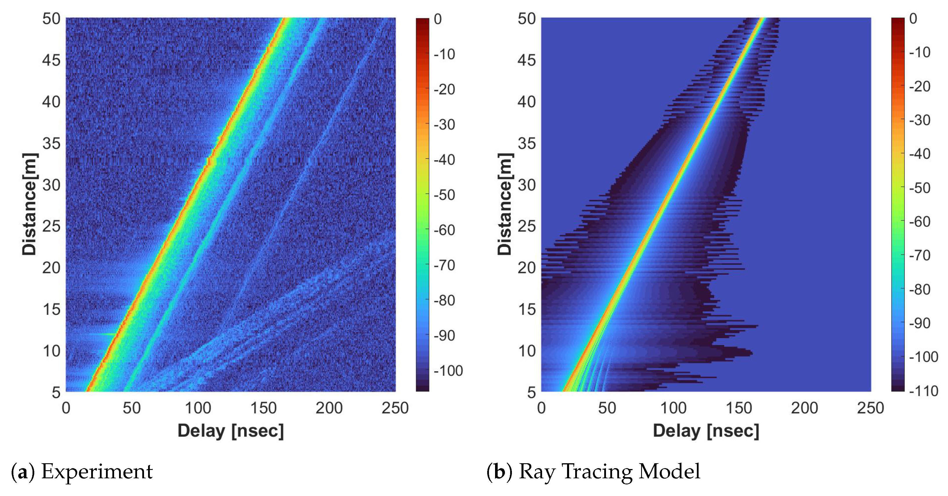
In order to obtain a broad observation of the tunnels’ influence on the wide-band communication, a 3D plot of the PDP throughout the tunnel is shown in Figure 9.

As can be observed in Figure 9, the LOS ray is absorbed at the receiver with a time suitable to the speed of light. This means that the LOS ray is received first at the receiver, followed by the rest of the rays which have been reflected multiple times off the walls of the tunnels. It can be recognized that the main phenomena remain commensurate along the tunnel, and with high similarity between the experiment and simulation.

As described in Section 2, the average delay and RMS delay spread were calculated with the data obtained from the experiment and simulation. A comparison between the experiment and simulation data is shown in

Table 7. Average and RMS delay spread for various distances.

Distance (m)	Mean Delay Spread $\overline{\mathit{\tau }}$ (ns)		RMS Delay Spread ${\mathit{\sigma }}_{\mathit{\tau }}$ (ns)
	Experiment	Simulation	Experiment	Simulation
5	$3.4$	$3.2$	$0.78$	$0.85$
10	$2.4$	$2.65$	$0.62$	$0.63$
20	$2.6$	$2.85$	$0.66$	$0.67$
45	$2.3$	$2.4$	$0.41$	$0.44$

.

The mean delay, $\overline{\tau }$, remains almost at the same value along the tunnel. The differences that can be noticed between the experiment and the model are within the resolution range of the measurement setup, as mentioned previously.

A parameter with a significant value in wide-band communication is the RMS delay spread, as defined in Equation (12). RMS delay spread can accurately convey the message of whether a communication link is possible in the current medium and distance [28]. The RMS delay spread is presented as a function of the distance between the Tx and Rx, as visible in Figure 10.

The RMS delay spread, ${\sigma }_{\tau }$, throughout the tunnel remains smaller than 1ns. The value of 1 ns is significantly lower than other typical values, as shown in Table 1, but is similar to the values obtained in comparable studies [14]. Since the time resolution in the experiment is 0.2ns and the value of the RMS delay spread is greater than that, the result obtained is accurate.

As noticeable, the RMS delay spread, ${\sigma }_{\tau }$, is not a constant value along the tunnel. As mentioned, the antennas that were used are directional. When the range between the transmitter and receiver is small, a small number of rays reach the receiving antenna, but in high scatter, due to the large difference in the optical paths.

The farther away from the transmitter the receiver progresses, the smaller the difference in the optical paths becomes and then the scatter becomes smaller.

However, due to the directional characteristics of the antenna, at some point, additional rays that bounced off the walls begin to reach the receiving antenna, increasing the RMS delay spread.

After this stage, as the distance between the transmitter and the receiver increases, the RMS delay spread, ${\sigma }_{\tau }$, dwindles down. The difference in the optical paths between the rays that do not experience strong decay becomes smaller, and the scattering from here on out becomes smaller. In other words, the rays that are reflected several times no longer reach the receiver with any significant power. The rays that remain powerful enough to get to the receiver are the rays that are reflected infrequently or not at all, and their travel time is similar to the time of the LOS ray.

A comparison between the average values along the whole tunnel of the experiment and the model is shown in

Table 8. Summary Results.

Parameter	Symbol	Experiment	Simulation
Spread Delay (ns)	${\sigma }_{\tau }$	0.55	0.54

.

6. Discussion and Conclusions

This study discusses an extensive measurement campaign that was carried out in a pedestrian tunnel, in which various parameters were measured, including the delay spread. The results of the measurements obtained were processed to show their enormous significance in characterizing the limitations of wireless communication in tunnels. The main feature of pedestrian tunnels is the fact that they are narrow and long in relation to their width and height. This unique characteristic affects the arrival time of the LOS ray in comparison to the time of arrival of the rays reflecting off the walls.

Using our theory, as described in Section 2, an analysis was made of the received power and the delays in the arrival of the signal at the receiver as a result of the distance between the transmitter and the receiver. To validate the model, a wide-band experiment was performed using a VNA, which provided us with high-resolution measurements. With the use of optical means, the ability to receive the signal accurately was achieved. The results were presented, in Section 4, in the form of a comparison with the results of the theory, and as can be observed there is an excellent fit.

One of the main characteristics of the pedestrian tunnel is that the RMS delay spread, ${\sigma }_{\tau }$, decreases along the tunnel. This can be explained by the fact that as the distance increases the rays returning from the walls have a lower power due to the attenuation created by the reflections from the wall. This is in contrast to the direct LOS ray, with the only effect on it being free space loss, which is lower. The sizes obtained, mean and RMS delay spread are of the same order of magnitude as the results obtained in previous studies that were performed in areas with similar topography. In contrast to the previous studies, this research is the most in-depth and comprehensive study of communication limitations in the pedestrian tunnel.

As was presented, there is a process of dispersion within the tunnel that is affected by Multi path, the effect of the dispersion on the communication channel may cause inter-symbol interference and should be considered in channel design.