An Efficient Two-Stage Receiver Base on AOR Iterative Algorithm and Chebyshev Acceleration for Uplink Multiuser Massive-MIMO OFDM Systems

Abstract

The massive multiple-input multiple-output systems (M-MIMO) and orthogonal frequency-division multiplexing (OFDM) are considered to be some of the most promising key techniques in the emerging 5G and advanced wireless communication systems nowadays. Not only are the benefits of applying M-MIMO and OFDM for broadband communication well known, but using them for the application of the Internet of Things (IoT) requires a large amount of wireless transmission, which is a developing topic. However, its high complexity becomes a problem when there are numerous antennas. In this paper, we provide an effective two-stage multiuser detector (MUD) with the assistance of the accelerated over-relaxation (AOR) iterative algorithm and Chebyshev acceleration for the uplink of M-MIMO OFDM systems to achieve a better balance between bit error rate (BER) performance and computational complexity. The first stage of the receiver consists of an accelerated over-relaxation (AOR)-based estimator and is intended to yield a rough initial estimate of the relaxation factor $\omega$, the acceleration parameter $\gamma$, and transmitted symbols. In the second stage, the Chebyshev acceleration method is used for detection, and a more precise signal is produced through efficient iterative estimation. Additionally, we call this proposed scheme Chebyshev-accelerated over-relaxation (CAOR) detection. Conducted simulations show that the developed receiver, with a modest computational load, can provide superior performance compared with previous works, especially in the MU M-MIMO uplink environments.

1. Introduction

Nowadays, the Internet of Things (IoT) of 5G [1,2,3] is one of the crucial applications of wireless communication systems [4,5,6]. Namely, wireless transmission services have become an extremely important method of Internet of Things (IoT) information delivery. The applications of the Internet of Things (IoT) include smart homes, healthcare, traffic auxiliary management, industrial automation, and crisis response for natural and artificial disaster prevention. To meet various types of applications of the Internet of Things (IoT), wireless transmission of large amounts of results to data collection centers is an essential need, i.e., 5G technology will be forced to bear massive amounts of data while being more time saving than 4G. Furthermore, the multiple-input multiple-output (MIMO) and the orthogonal frequency-division multiplexing (OFDM) are indispensable technologies of wireless communication systems currently [7,8]. The former, with multiple antennas at the transmitters and receivers, which can significantly increase the data throughput of the system and transmission distance without increasing the total transmit power expenditure or bandwidth demand, also can efficiently obtain diversity gain, array gain, capacity gain, and beamforming gain [9,10,11]; the latter is a favored modulation and transmission scheme that cuts a high-data-rate stream into some lower-rate streams simultaneously transmitted over some narrow-band channels parallelly, which has a lot of advantages, such as robustness against narrow-band co-channel interference, inter-symbol interference (ISI) caused by multipath propagation, and low sensitivity to time synchronization errors [12,13]. To further promote the merits of the MIMO systems and meet higher spectrum efficiency, the pioneer researchers proposed the massive MIMO (M-MIMO) structure [14,15,16,17], which utilizes spatial diversity to support more users by mounting a large number of antennas in the base station (BS) [18,19,20].

It is a pity that, although the M-MIMO systems have brought many benefits, complexity is also appreciably increased. Especially as far as the receiver is concerned, conventional linear detection methods such as zero-forcing (ZF) and minimum mean-square error (MMSE) are adopted [21,22], even if they show good bit error rate (BER) performance; however, as mentioned by Yin et al. [23], since they involve matrix inversion operations of $\mathcal{O}(N^3)$ complexity, the detection complexity is too high to implement when N is increasing, where N is the antenna number.

Therefore, many iterative methods aim to eschew matrix inversion and not calculate it. In addition, a comparative study of low-complexity linear detectors of M-MIMO is addressed in [24] to discuss the pros and cons of iterative matrix inversion methods. To maintain good performance and low complexity, low-complexity signal detection for the uplink of massive MIMO systems is proposed, such as the Jacobi method [25], Gauss–Seidel method [26], and successive over-relaxation (SOR) method [27] proposed by Kong et al., Wu et al., and Gao et al., respectively, which have lower complexity as $\mathcal{O}(N^2)$ through the iterative procedure to avoid the notorious inverse matrix operation. However, the performance is not sufficient to satisfy us. In light of this, Yu et al. [28] considered a modified SOR method to reduce the complexity, but it is strongly confined to lower modulation orders; namely, its performance degrades substantially when the high modulation order becomes more required. In [29], Ning et al. proposed the symmetric successive over-relaxation (SSOR) method, which combines two SOR sweeps in such a way that the resulting iteration matrix is similar to a symmetric matrix and its performance is better than the previous SOR-based method; nevertheless, its complexity will increase drastically compared to the SOR-based method. Compared to the SOR-based method [27], Zhang et al. proposed the AOR method in [30], which is an extension of the SOR by using two parameters to speed up convergence, though the complexity of AOR is slightly higher than SOR; however, its performance can be significantly improved. To obtain a reasonable computational load, the Chebyshev acceleration uses the extension of the extrapolation acceleration method to accelerate convergence and reduce complexity [31].

In light of the above, to achieve a good trade-off between BER performance and complexity load, we propose a two-stage receiver for the MU M-MIMO systems, called Chebyshev-accelerated over-relaxation (CAOR) detection. The first stage of the receiver consists of setting each parameter of the AOR method [30] and using its algorithm to produce the rough initial estimate outputs, and then submitting those initial estimates of symbol detection and the AOR parameters to the second stage. In the second stage, the Chebyshev acceleration is conducted successively using the recursive relationship of the Chebyshev polynomials. It is noteworthy that, to render the estimated parameters more thoroughly, unlike the conventional iterative algorithm, this method provides Chebyshev algorithm calculation through AOR’s initial estimated output and parameters to produce more precise and fast signal detection. Conducted simulations show that the proposed two-stage detection scheme, with a modest computational load, can provide superior performance compared with most iterative detection methods, especially in uplink MU M-MIMO scenarios.

The rest of this paper is organized as follows. Section 2 introduces the system model employed in this paper. A review of some conventional iterative schemes and a new two-stage receiver based on the AOR iterative algorithm and Chebyshev acceleration are addressed in Section 3. Simulation results and computational complexity analysis are provided in Section 4 to verify the proposed approach. Section 5 provides the concluding remarks to summarize the paper.

2. System Model

2.1. Uplink Multiuser MIMO OFDMA Systems

We consider the uplink multiuser MIMO orthogonal frequency-division multiple access (OFDMA) systems [32,33] with $K{N}_t$ user antennas, and $N_R$ antennas at the BS, where K is the user number, each user is equipped with $N_t$ transmit antennas, and $N_R\gg K{N}_t$. Then, we use $N_T$ to represent the total number of user antennas. The transmitted signal and the received signal can be expressed as $\mathbf{s}={[s_1,s_2,\cdots ,s_{N_T}]}^T$ and $\mathbf{y}={[y_1,y_2,\cdots ,y_{N_R}]}^T$, respectively. In addition, we use bold and capitals to denote vector and matrix, respectively. Hence, the system model can be represented by the following Equation (1):

$$\mathbf{y}=H\mathbf{s}+\mathbf{n},$$

(1)

where H is the $N_R\times N_T$ complex channel matrix and $\mathbf{n}$ is the $N_R\times 1$ noise vector. Moreover, it can be expressed as

$$\left[\begin{array}{c}{y}_1\\ ⋮\\ y_{N_R}\end{array}\right]=\left[\begin{array}{ccc}{h}_{11}& \cdots & h_{1N_T}\\ ⋮& \ddots & ⋮\\ h_{N_{R}1}& \cdots & h_{N_R{N}_T}\end{array}\right]\left[\begin{array}{c}{s}_1\\ ⋮\\ s_{N_T}\end{array}\right]+\left[\begin{array}{c}{n}_1\\ ⋮\\ n_{N_R}\end{array}\right].$$

(2)

2.2. Channel Model

We assume that $H\in {\mathbb{C}}^{N_R\times N_T}$ denotes the flat Rayleigh fading channel matrix with two-channel taps that are independent and identically distributed (i.i.d.) and obey Gaussian distribution with unit variance and zero mean, and the elements in noise vector $\mathbf{n}$ are i.i.d. and have complex Gaussian distribution $\mathcal{C}\mathcal{N}\left(0,{\sigma }^2\right)$.

At the BS, the task of the detector is to estimate the transmitted signal vector $\mathbf{s}$ from the received signal vector $\mathbf{y}$. According to [20], the conventional linear MMSE detection algorithm has been proven, which is near-optimal for uplink MIMO systems. In addition, the estimate of the transmitted signal vector $\mathbf{s}$ can be expressed as

$$\mathbf{s}={(H^{H}H+{\sigma }^2{I}_{N_T})}^{-1}{H}^H\mathbf{y}=W^{-1}{\mathbf{y}}^{MF},$$

(3)

where ${\sigma }^2$ denotes the variance of the noise vector, W is the filtering matrix of conventional MMSE, and ${\mathbf{y}}^{MF}$ is the output of the matched filter. Within Equation (3), we can observe that the matrix inversion operation is contained in the conventional MMSE detection. Therefore, the computational complexity of conventional MMSE is too high to realize in the MU-MIMO systems, not to mention the massive antennas.

To estimate the flat Rayleigh fading matrix at the BS, we used a comb-type pilot structure [34], with pilot tones at periodically located subcarriers. Then, we used the least square (LS) channel estimation method [35] to find the channel estimate ${\widehat{H}}_{LS}$ by pilot tones. The result of LS channel estimation is given by [7]

$${\widehat{H}}_{LS}={(X^{H}X)}^{-1}{X}^{H}Y=X^{-1}Y,$$

(4)

where X and Y denote the transmitted signal’s pilot tones and the received signal’s pilot tones at the subcarriers, respectively.

3. Proposed Scheme

To explain our proposed method more clearly, first, we will briefly describe the conventional SOR method [27], AOR method [30], and Chebyshev acceleration method [31], sequentially, and then propose a two-stage CAOR scheme to balance the performance and complexity trade-off by performing fewer iterations to further accelerate convergence.

3.1. Iteration Method Review

3.1.1. Conventional SOR Method

We consider a linear system [36] whose mathematical equation can be expressed as

$$A\mathbf{x}=\mathbf{b},$$

(5)

where the matrix A is symmetric positive-definite, $\mathbf{x}$ is the unknown vector and we can decompose A as follows:

$$A=D-L-U,$$

(6)

in which D, $-L$, and $-U$ are the diagonal, strict lower part, and strict upper part of A. As for the iterative equation, the Jacobi iteration [25] is given by

$${\mathbf{x}}^{(k+1)}=D^{-1}(L+U){\mathbf{x}}^{(k)}+D^{-1}\mathbf{b},$$

(7)

Likewise, the Gauss–Seidel iteration [26] also can be expressed as

$${\mathbf{x}}^{(k+1)}={(D-L)}^{-1}U{\mathbf{x}}^{(k)}+{(D-L)}^{-1}\mathbf{b}.$$

(8)

Here, we can define a matrix G as

$$G=M^{-1}N.$$

(9)

Therefore, for the Jacobi iteration, $M=D$ and $N=(L+U)$. Moreover, for the Gauss–Seidel iteration, $M=(D-L)$ and $N=U$. Then, Equations (7) and (8) can be rewritten as

$${\mathbf{x}}^{(k+1)}=G{\mathbf{x}}^{(k)}+\mathbf{d},$$

(10)

where G is called the iteration matrix and $\mathbf{d}$ is $M^{-1}\mathbf{b}$. Based on this result, we multiply the relaxation factor $\omega$ in Equation (10), and we have

$$\omega {\mathbf{x}}^{(k+1)}=\omega (G{\mathbf{x}}^{(k)}+\mathbf{d}),$$

(11)

which gives the SOR iteration [27]. Take the Gauss–Seidel iteration as an example, which is defined as

$${\mathbf{x}}^{(k+1)}={(D-\omega L)}^{-1}\left\{[(1-\omega )D+\omega U]{\mathbf{x}}^{(k)}+\omega \mathbf{b}\right\}.$$

(12)

According to [27], we can determine that the SOR iterative algorithm is convergent.

3.1.2. AOR Method

The accelerated over-relaxation (AOR) iterative algorithm [37] can be regarded as an extension of the successive over-relaxation (SOR) iterative algorithm, and its iterative equation is as follows:

$$\begin{array}{cc}\hfill {\mathbf{x}}^{(k+1)}& ={(D-\gamma L)}^{-1}[(1-\omega )D+\omega U+(\omega -\gamma )L]{\mathbf{x}}^{(k)}\hfill \\ \hfill & +\omega {(D-\gamma L)}^{-1}\mathbf{b},\hfill \end{array}$$

(13)

where $\omega$ and $\gamma$ are the relaxation parameter and the acceleration parameter, respectively. Furthermore, for specific values of $\omega$ and $\gamma$, when $\omega =\gamma$ or $\omega =\gamma =1$, the AOR iterative algorithm can reduce to the SOR or the Gauss–Seidel iterative algorithm, respectively.

According to $Lemma$ 1 in [27], in uplink large-scale MIMO, the conventional MMSE filtering matrix W is a symmetric positive definite matrix, and it can be decomposed as

$$W=D+L+L^H.$$

(14)

where D, L, and $L^H$ are the diagonal, strict lower part, and strict upper part of W. Therefore, we can use the AOR iterative algorithm to rewrite the conventional MMSE algorithm as follows:

$$\begin{array}{cc}\hfill {\mathbf{x}}^{(k+1)}& ={(D+\gamma L)}^{-1}[(1-\omega )D-\omega L^H-(\omega -\gamma )L]{\mathbf{x}}^{(k)}\hfill \\ \hfill & +\omega {(D+\gamma L)}^{-1}{\mathbf{y}}^{MF},\hfill \end{array}$$

(15)

and the relaxation parameter $\omega$ and the acceleration parameter $\gamma$ of the AOR iterative method are given by [37] as follows:

$$\begin{array}{ccc}\hfill \omega & =& \frac{1}{\sqrt{1-{\mu }^2}},\hfill \end{array}$$

(16)

$$\begin{array}{ccc}\hfill \gamma & =& \frac{2}{1+\sqrt{1-{\mu }^2}},\hfill \end{array}$$

(17)

where $\mu ={\left.\rho (G_{\gamma ,\omega })\right|}_{\gamma =0,\omega =1}$; we will also define $\rho (G_{\gamma ,\omega })$ in later sections.

AOR Convergence Analysis

We know that in any iterative algorithm in the form of Equation (10), when k reaches infinity, ${\mathbf{x}}^{(k+1)}$ will be equal to ${\mathbf{x}}^{(k)}$. Noting Equation (15), we can use Equation (10) to define $G_{\gamma ,\omega }={(D+\gamma L)}^{-1}[(1-\omega )D-\omega L^H-(\omega -\gamma )L]$ and $\mathbf{d}=\omega {(D+\gamma L)}^{-1}{\mathbf{y}}^{MF}$; afterward, Equation (15) can be rewritten as

$${\mathbf{x}}^{(k+1)}=G_{\gamma ,\omega }{\mathbf{x}}^{(k)}+\mathbf{d},$$

(18)

and the spectral radius of $G_{\gamma ,\omega }$ is defined as the non-negative number as follows:

$$\rho (G_{\gamma ,\omega })\triangleq \underset{\lambda \in \rho (G_{\gamma ,\omega })}{max}\left|\lambda \right|,$$

(19)

in which $\lambda$ is the eigenvalue of $G_{\gamma ,\omega }$. Moreover, if the spectral radius $\rho (G_{\gamma ,\omega })$ satisfies

$$\rho (G_{\gamma ,\omega })=\underset{1<n<N_T}{max}\left|{\lambda }_n\right|<1,$$

(20)

Therefore, Equation (15) will converge [31]. According to the theorem of eigenvalues, we can obtain

$$G_{\gamma ,\omega }\mathbf{x}={(D+\gamma L)}^{-1}[(1-\omega )D-\omega L^H-(\omega -\gamma )L]\mathbf{x}={\lambda }_n\mathbf{x},$$

(21)

where $\mathbf{x}$ is an arbitrary $N_T\times 1$ non-zero real-valued vector and Equation (21) also can be rewritten as

$$[(1-\omega )D-\omega L^H-(\omega -\gamma )L]\mathbf{x}=(D+\gamma L){\lambda }_n\mathbf{x}.$$

(22)

Multiplying both sides of Equation (22) by the conjugate transpose of $\mathbf{x}$, we can obtain

$${\mathbf{x}}^H[(1-\omega )D-\omega L^H-(\omega -\gamma )L]\mathbf{x}={\mathbf{x}}^H(D+\gamma L){\lambda }_n\mathbf{x}.$$

(23)

Next, we take the conjugate transpose on both sides of Equation (23), in which D is a diagonal matrix, so $D=D^H$, and then we can obtain an updated equation as

$${\mathbf{x}}^H[(1-\omega )D-\omega L-(\omega -\gamma )L^H]\mathbf{x}={\mathbf{x}}^H(D+\gamma L^H){\lambda }_n\mathbf{x}.$$

(24)

Then, adding Equations (23) and (24) will obtain

$$\begin{array}{cc}\hfill & {\mathbf{x}}^H[(2-2\omega )D-\omega (L+L^H)-(\omega -\gamma )(L+L^H)]\mathbf{x}\hfill \\ \hfill & ={\mathbf{x}}^H{\lambda }_n[2D+\gamma (L+L^H)]\mathbf{x}.\hfill \end{array}$$

(25)

Substituting Equation (14) into Equation (25), we can obtain

$$({\lambda }_n-1)(\gamma -2){\mathbf{x}}^{H}D\mathbf{x}=[{\lambda }_n\gamma +(2\omega -\gamma )]{\mathbf{x}}^{H}W\mathbf{x},$$

(26)

Since the filter matrix W of conventional MMSE is positive definite, as demonstrated in [27], D is also positive definite, i.e., the diagonal matrix of W. Thus, we have ${\mathbf{x}}^{H}D\mathbf{x}>0$ and ${\mathbf{x}}^{H}W\mathbf{x}>0$. Moreover, if both $(\gamma -2)$ and $({\lambda }_n-1)$ are less than zero, i.e., $0<\gamma <2$ and ${\lambda }_n<1$, then

$$({\lambda }_n-1)(\gamma -2)>0,$$

(27)

and ${\lambda }_n\gamma +(2\omega -\gamma )>0$. Therefore, we can determine that $({\lambda }_n-1)[{\lambda }_n\gamma +(2\omega -\gamma )]<0$, that means

$${\lambda }_n[({\lambda }_n-2)\gamma +2\omega ]<2\omega -\gamma .$$

(28)

We know that when $\omega =\gamma$, we can obtain

$$\left|{\lambda }_n\right|<1.$$

(29)

Paying attention to Equation (29), if we give appropriate values of $\omega$ and $\gamma$, it can be guaranteed to comply with $\rho (G_{\gamma ,\omega })<1.$ Thus, the AOR iterative algorithm is convergent.

3.1.3. Chebyshev Acceleration

Chebyshev acceleration [31] can be regarded as the promotion of extrapolation acceleration. Consider ${\mathbf{x}}^{(0)},{\mathbf{x}}^{(1)},\dots ,{\mathbf{x}}^{(k)}$, if ${\epsilon }_k={\mathbf{x}}^{(k)}-{\mathbf{x}}^{\ast }$ is defined as the error of the kth iteration solution, in which ${\mathbf{x}}^{\ast }$ is a target signal and ${\mathbf{x}}^{(k)}$ is kth-time iteration output; then, ${\epsilon }_k$ can be expressed as

$${\epsilon }_k=G{\epsilon }_{k-1}=G^2{\epsilon }_{k-2}=\cdots =G^k{\epsilon }_0,$$

(30)

where G is the iteration matrix and $G^k$ is kth-time iteration matrix. Assume that ${\tilde{\mathbf{x}}}^{(k)}$ is the linear combination of ${\mathbf{x}}^{(0)},{\mathbf{x}}^{(1)},\dots ,{\mathbf{x}}^{(k)}$ as follows

$${\tilde{\mathbf{x}}}^{(k)}={\alpha }_0{\mathbf{x}}^{(0)}+{\alpha }_1{\mathbf{x}}^{(1)}+\cdots +{\alpha }_k{\mathbf{x}}^{(k)},$$

(31)

where ${\alpha }_k$ is undetermined coefficients, and it satisfies ${\sum }_{i=0}^k{\alpha }_i=1$. Therefore, ${\tilde{\mathbf{x}}}^{(k)}-{\mathbf{x}}^{\ast }$ can be defined as

$${\tilde{\mathbf{x}}}^{(k)}-{\mathbf{x}}^{\ast }={\alpha }_0{\epsilon }_0+{\alpha }_{1}G{\epsilon }_0+\cdots +{\alpha }_k{G}^k{\epsilon }_0\triangleq p_k(G){\epsilon }_0,$$

(32)

in which $p_k(G)={\sum }_{i=0}^k{\alpha }_i{G}^i$ is a k-degree polynomial, and it satisfies $p_k(I)=I$. We look forward to choosing the appropriate coefficients ${\alpha }_i$ to let ${\tilde{\mathbf{x}}}^{(k)}-{\mathbf{x}}^{\ast }$ be as small as possible and increase the convergence rate. Obviously, this is an optimization problem. According to the definition in Equation (32), we can obtain

$${∥{\tilde{\mathbf{x}}}^{(k)}-{\mathbf{x}}^{\ast }∥}_2={∥p_k(G){\epsilon }_0∥}_2\le {∥p_k(G)∥}_2·{∥{\epsilon }_0∥}_2,$$

(33)

then, we need to solve the minimization problem below

$$\begin{array}{c}\hfill \underset{p_k\in P_k,p_k(I)=I}{min}{∥p_k(G)∥}_2,\end{array}$$

(34)

in which $P_k$ is the set of all polynomials, where the capital P stands for polynomials and the lowercase k stands for the maximum degree. To solve the above problem, in particular, we assume that the iteration matrix G is a symmetric matrix, which means that G has the spectral decomposition as follows:

$$G=Q\Lambda Q^T,$$

(35)

where $\Lambda$ is a diagonal matrix and Q is an orthogonal matrix; therefore,

$$\begin{array}{cc}\hfill \underset{p_k\in P_k,p_k(I)=I}{min}{∥p_k(G)∥}_2& =\underset{p_k\in P_k,p_k(I)=I}{min}{∥p_k(\Lambda )∥}_2\hfill \\ \hfill & =\underset{p_k\in P_k,p_k(I)=I}{min}\underset{1\le i\le n}{max}\left\{\left|p_k({\lambda }_i)\right|\right\}\hfill \\ \hfill & =\underset{p_k\in P_k,p_k(I)=I}{min}\underset{\lambda \in [{\lambda }_n,{\lambda }_1]}{max}\left\{\left|p_k(\lambda )\right|\right\},\hfill \end{array}$$

where ${\lambda }_n$ and ${\lambda }_1$ are the maximum and the minimum eigenvalue, respectively. Next, we consider the iteration equation, Equation (10), in which the eigenvalues of the iteration matrix G are all real numbers, the iterative matrix spectral radius $\rho =\rho (G)<1$ and $\lambda \in [-\rho ,\rho ]\subset (-1,1)$. Thus, Equation (36) can be converted into

$$\underset{p_k\in P_k,p_k(I)=I}{min}\underset{\lambda \in [-\rho ,\rho ]}{max}\left\{\left|p_k(\lambda )\right|\right\}.$$

(36)

According to the above result, we can follow the Chebyshev polynomials’ properties [31] to solve Equation (37) as follows:

$$p_k(t)=\frac{T_k(t/\rho )}{T_k(1/\rho )},$$

(37)

where $T_k(t)$ is the k-degree Chebyshev polynomials. In fact, we can use the recurrence relation of the Chebyshev polynomials as follows:

$$T_k(t)=2t{T}_{k-1}(t)-T_{k-2}(t),k=2,3,\dots ,$$

(38)

in addition, let ${\mu }_k=\frac{1}{T_k(1/\rho )}$ or ($T_k(1/\rho )=\frac{1}{{\mu }_k}$), and we can obtain a new recurrence relation equation as

$$\frac{1}{{\mu }_k}=\frac{2}{\rho }·\frac{1}{{\mu }_{k-1}}-\frac{1}{{\mu }_{k-2}}.$$

(39)

Substituting Equation (40) into Equation (32), we can obtain

$${\tilde{\mathbf{x}}}^{(k)}=\frac{2{\mu }_k}{{\mu }_{(k-1)}}·\frac{G}{\rho }{\tilde{\mathbf{x}}}^{(k-1)}-\frac{{\mu }_k}{{\mu }_{(k-2)}}{\tilde{\mathbf{x}}}^{(k-2)}+\frac{2{\mu }_k}{{\mu }_{(k-1)}\rho }\mathbf{d}.$$

(40)

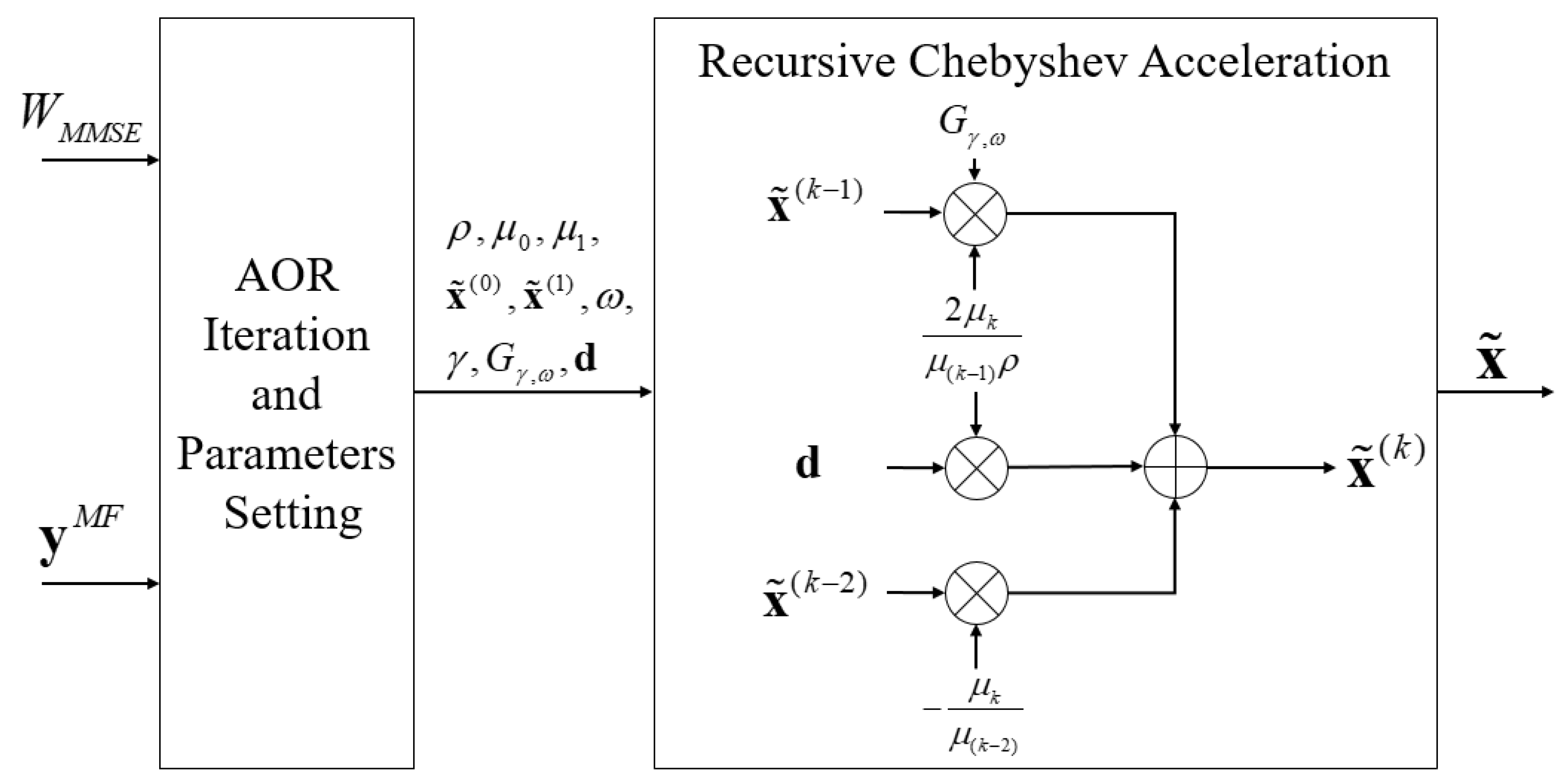
3.2. Proposed CAOR Method

In light of the previous subsections, to improve the BER performance and alleviate the significant complexity, we joined the AOR iterative algorithm and the recursive characteristics of the Chebyshev polynomials to construct a two-stage receiver, as depicted in Figure 1, in which the second block has more apparently depicted the Chebyshev recursive procedure. It can speed up convergence with fewer iterations and produce better estimation results. Additionally, we call this proposed scheme Chebyshev-accelerated over-relaxation (CAOR) detection.

The first stage of the receiver is an initial phase, which consists of an accelerated over-relaxation (AOR)-based estimator and is intended to yield a rough initial estimate of the relaxation factor $\omega$, the acceleration parameter $\gamma$, the spectral radius of $G_{\gamma ,\omega }$, and transmitted symbols. The second stage is a refined phase, the Chebyshev acceleration method is used for detection, and a more precise signal is produced through efficient iterative estimation. The procedure of the CAOR detection is shown in Algorithm 1.

Algorithm 1 Chebyshev-Accelerated Over-Relaxation

Receiver signal input: 1.  $W_{MMSE}=H^{H}H+{\sigma }^2{I}_{N_T}\triangleq A$, and $A=D+L+L^H$ 2.  ${\mathbf{y}}^{MF}=H^H\mathbf{y}\triangleq \mathbf{b}$ The first stage: (Initialize phase) 1.  $G_{\gamma ,\omega }={(D+\gamma L)}^{-1}[(1-\omega )D-(\omega -\gamma )L-\omega L^H]$ 2.  $\mathbf{d}=\omega {(D+\gamma L)}^{-1}\mathbf{b}$ 3.  set $\rho =\rho (G_{0,1})$, $\rho (G_{\gamma ,\omega })$ is the spectral radius of $G_{\gamma ,\omega }$ 4.  set ${\mu }_0=1$, ${\mu }_1=\rho$, ${\tilde{\mathbf{x}}}^{(0)}={\mathbf{x}}^{(0)}=\mathbf{1}$ and $k=1$      Compute $\omega =\frac{1}{\sqrt{1-{\mu }_1^2}},\gamma =\frac{2}{1+\sqrt{1-{\mu }_1^2}}$      Compute ${\mathbf{x}}^{(1)}=G_{\gamma ,\omega }{\mathbf{x}}^{(0)}+\mathbf{d}\triangleq {\tilde{\mathbf{x}}}^{(1)}$ The second stage: (Refined phase) While not converge do 1.  $k=k+1$ 2.  ${\mu }_k={(\frac{2}{\rho }·\frac{1}{{\mu }_{k-1}}-\frac{1}{{\mu }_{k-2}})}^{-1}$ 3.  ${\tilde{\mathbf{x}}}^{(k)}=\frac{2{\mu }_k}{{\mu }_{(k-1)}}·\frac{G_{\gamma ,\omega }}{\rho }{\tilde{\mathbf{x}}}^{(k-1)}-\frac{{\mu }_k}{{\mu }_{(k-2)}}{\tilde{\mathbf{x}}}^{(k-2)}+\frac{2{\mu }_k}{{\mu }_{(k-1)}\rho }\mathbf{d}$ end set $\tilde{\mathbf{x}}={\tilde{\mathbf{x}}}^{(k)}$ Receiver signal output: The estimate of the transmitted signal vector $\tilde{\mathbf{x}}$

4. Simulation Results and Complexity Analysis

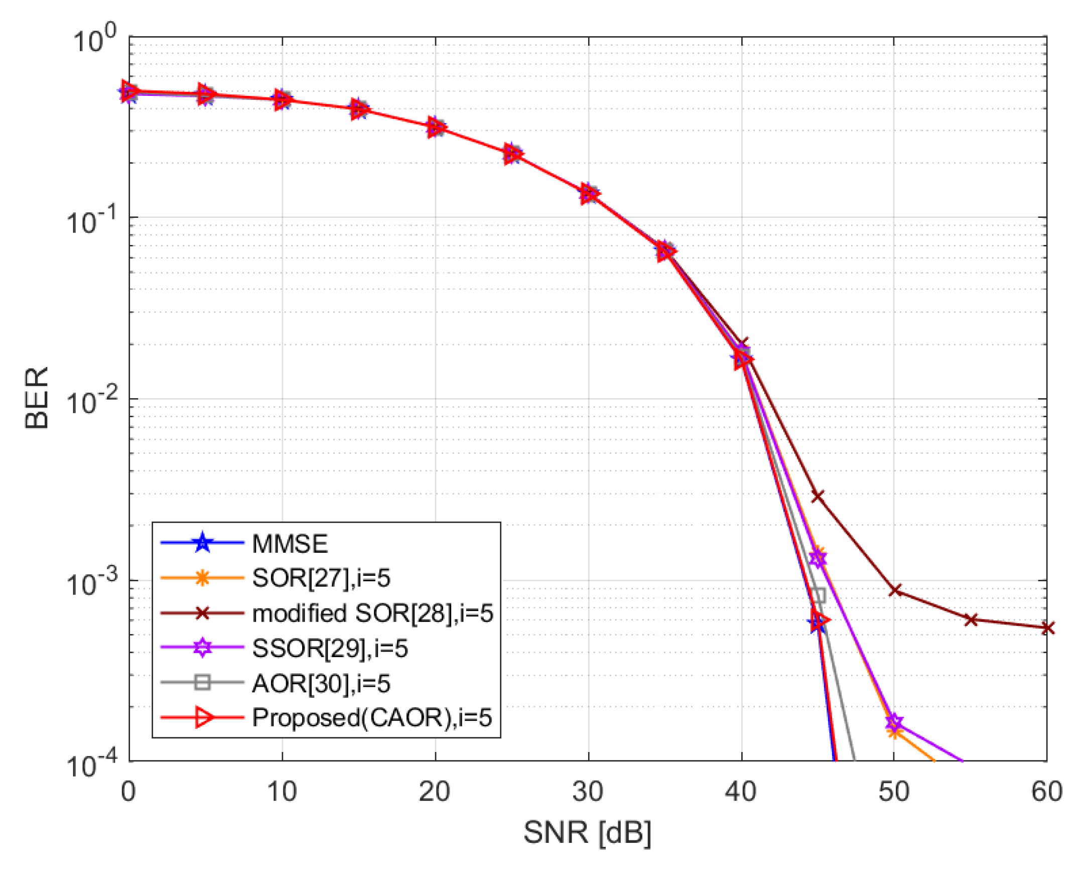
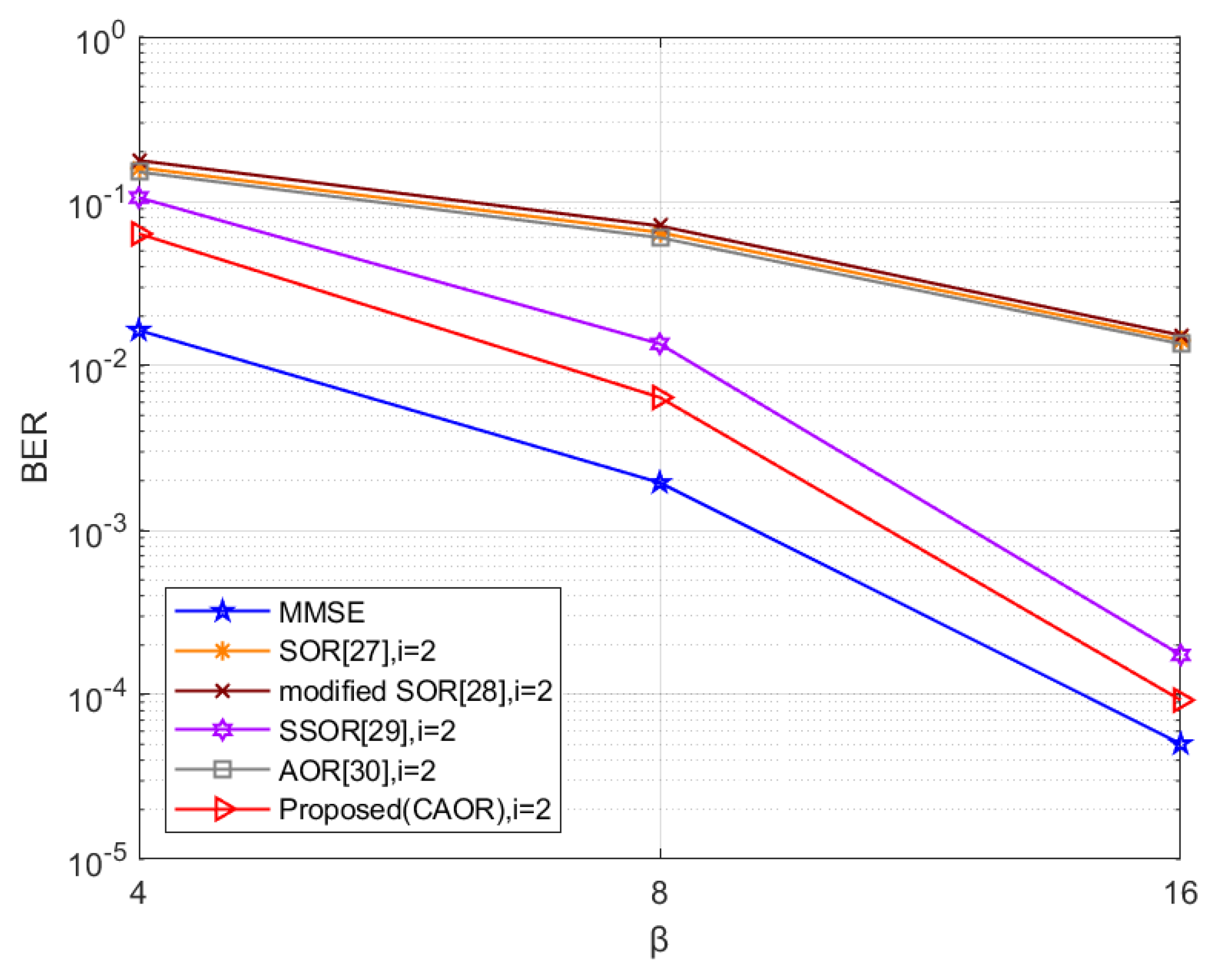
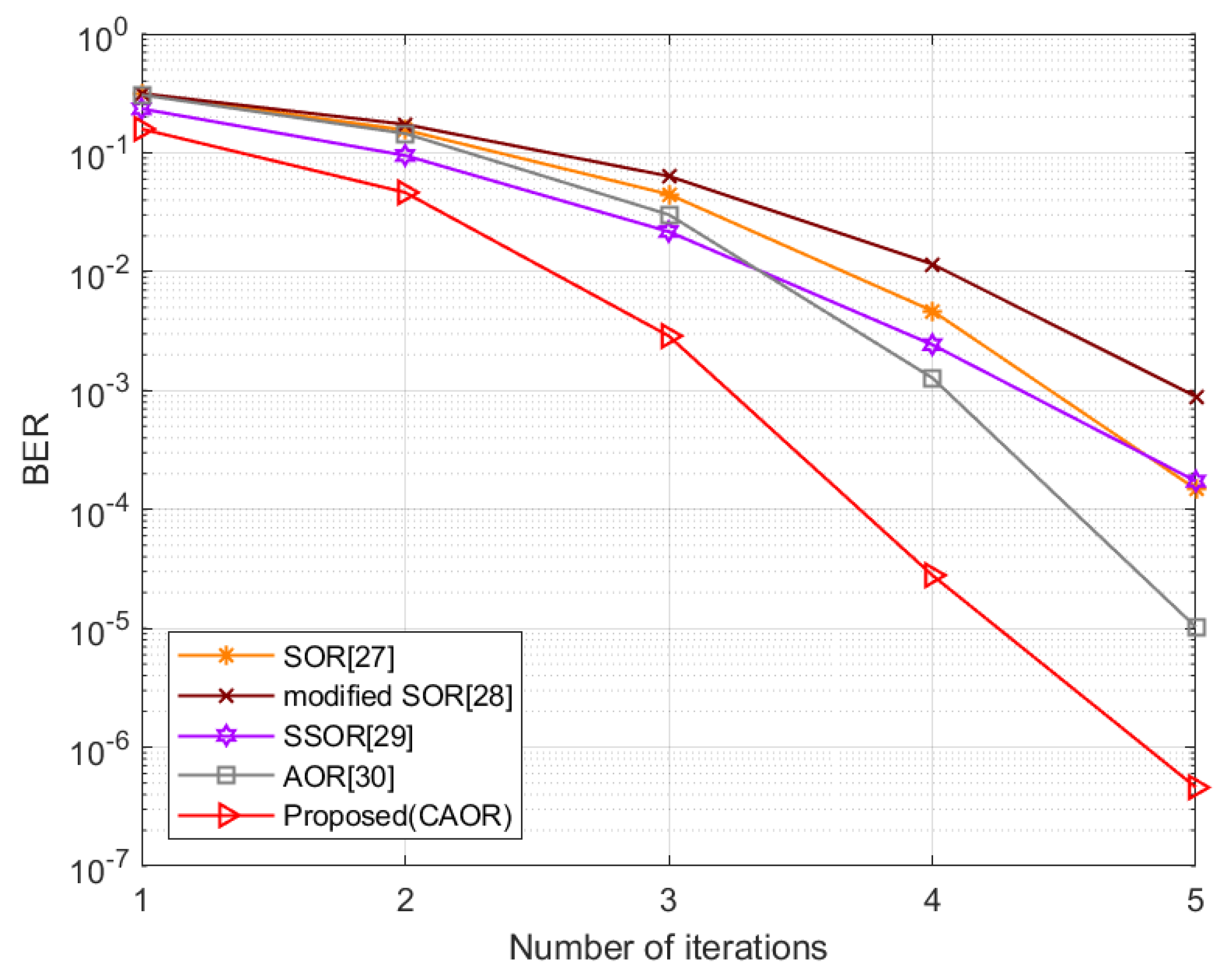
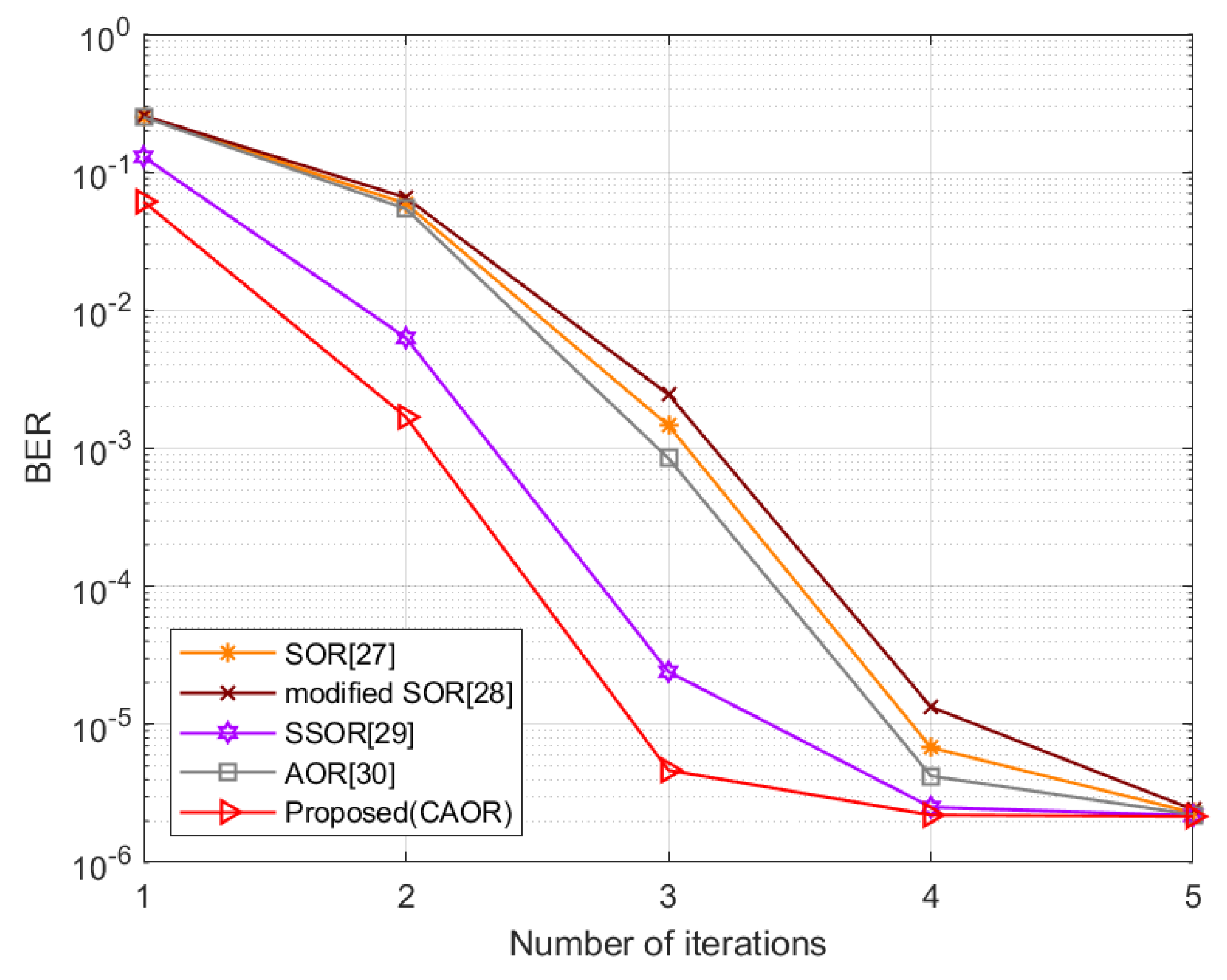
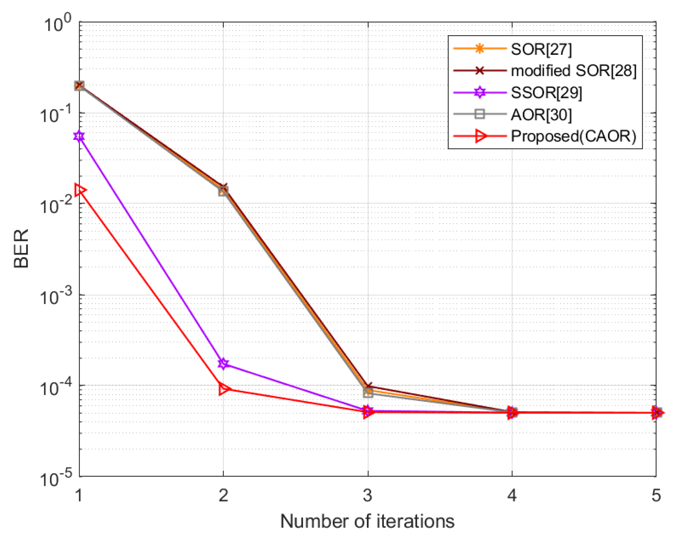
4.1. Simulation Results and Discussion

Some numerical simulations are conducted to evaluate the performance of the proposed two-stage receiver. Consider an $N_R\times N_T$ uplink MU M-MIMO OFDMA systems as depicted in Section 2, where $N_R$ and $N_T$ are the numbers of the antennas at the base station side and total user side, respectively. As in

Table 1. Simulation scenarios.

System	Parameter
Number of data subcarriers	256
Number of OFDM symbols	100
Modulation scheme	1024-QAM
CP Length	64
Number of pilot data in one OFDM symbol	20
The maximum SNR	60
Channel	Rayleigh fading channel
Number of channel taps	2
Noise	AWGN
Channel estimation	LS
Monte Carlo (times)	10,000

, simulation scenarios are 1024-quadrature amplitude modulation (QAM) and the number of subcarriers as 256, 100 OFDM symbols, cyclic prefix (CP) length is 64, each symbol has pilots as 20. In addition, assume that the channels are two-ray flat Rayleigh fading with additive white Gaussian noise (AWGN) and channel state information (CSI) is available at the receiver by LS estimation. Five receivers, including the SOR [27], the modified SOR [28], the SSOR [29], the AOR [30], and the proposed two-stage receiver, are conducted for comparison in terms of the bit error rate (BER) performance. Moreover, to accentuate the novelty of our proposed scheme, we briefly describe the characteristics of previously published work and our proposed scheme in

Table 2. A brief comparison of our proposed scheme and previously published work.

Scheme	Brief Description
SOR [27]	SOR is a method of solving a linear system of equations derived by extrapolating the Gauss–Seidel method.
modified SOR [28]	Modified SOR is a variant of SOR, which changes certain parameters in the SOR algorithm and is nearly unaffected by the relaxation factor $\omega$ in lower modulation order.
SSOR [29]	SSOR combines two SOR sweeps in such a way that the resulting iteration matrix is similar to a symmetric matrix.
AOR [30]	The AOR iterative algorithm can be regarded as an extension of the SOR iterative algorithm, which is a two-parameter generalization of the SOR method.
CAOR	The CAOR method combines the AOR iterative algorithm and the recursive characteristics of the Chebyshev polynomials.

.

First, we use Equations (16) and (17) to gain the appropriate relaxation parameter $\omega$ and the acceleration parameter $\gamma$, respectively, within the first stage. Apart from this, we show the BER performance of the proposed CAOR scheme against $\gamma$ and $\omega$ for different relaxation parameter $\omega$ values and acceleration parameter $\gamma$ values in Figure 2 and Figure 3, respectively, when the number of iterations i is 4, $N_R\times N_T=64\times 16$ and the SNR level is set to 40 dB. We can observe that if $\omega$ approaches 1.1 or so, the BER performance will improve; otherwise, BER performance will decrease. Thus, we believe that the choice of $\omega$ close to 1.1 and $\gamma$ close to 1.0 will yield the best parameter estimate. Simultaneously, the inferences from Figure 2 and Figure 3 are consistent with the calculated values of Equations (16) and (17), respectively.

Figure 4, Figure 5 and Figure 6 depict the BER performance comparison with five different detection schemes, and $N_R$ is 64, 128, and 256, respectively. In Figure 4, we can roughly observe that the CAOR method is closest to the performance of conventional MMSE when the iteration number is equal to five. Moreover, when SNR = 45 dB, the BER performance of CAOR and AOR is approximately $0.6\times {10}^{-3}$ and $0.8\times {10}^{-3}$, respectively. In other words, compared to AOR, CAOR can improve BER performance by 25%.

When increasing $N_R$ to 128 and the number of iterations i is 3, shown in Figure 5, we continued to observe that the BER performance of the proposed method almost overlaps with the conventional MMSE scheme, only requiring three iterations. Moreover, Figure 6 shows that when $N_R$ increases to 256 and is iterated twice only, we can note that the proposed method has the best BER performance in comparison with other detectors.

We turn now to the ratio ($\beta$) analysis, which is the ratio between the number of base station antennas ($N_R$) and the total number of user antennas ($N_T$) [24]. As shown in Figure 7, the BER performance changes in terms of the $\beta$ of each detection scheme. Alongside this, when $\beta$ equals 16 and SNR is 40 dB, the BER performance of SSOR and CAOR is equal to $1.75\times {10}^{-4}$ and $9.27\times {10}^{-5}$, respectively. Taking it for granted, relative to the higher $\beta$ value, the BER performance of all detectors is improved due to the spatial diversity gain of a large number of antennas without exception. Moreover, we know that, regardless of the $\beta$ value, for the BER performance, SSOR is satisfactory, as is AOR, but our proposed scheme CAOR surpasses them all.

It is worth mentioning that when the number of antennas continues to increase, the number of iterations required is relatively reduced; simultaneously, the BER performance of our proposed method improves more definitely. On the whole, this is a good result for a 5G system with massive antennas.

Moreover, in

Table 3. Comparison of the degree to which the BER performance approaches that of conventional MMSE among all detectors in terms of dB value under different $\beta$ as i = 2 and SNR at 40 dB.

Scheme	$\mathit{\beta }=4$	$\mathit{\beta }=8$	$\mathit{\beta }=16$
SOR	9.43 dB	15.19 dB	24.52 dB
modified SOR	9.91 dB	15.60 dB	24.82 dB
SSOR	7.34 dB	7.89 dB	3.93 dB
AOR	9.13 dB	14.86 dB	24.30 dB
CAOR	4.58 dB	3.74 dB	−0.738 dB

, we compare the degree of the BER performance approaching conventional MMSE among all detectors in terms of dB value (i.e., to obtain a more demarcated numerical comparison, we have taken $10log(·)$ for the BER distance between the individual detector and conventional MMSE) under different $\beta$, where the CAOR method has the smallest distance with conventional MMSE. Apart from this, when $\beta$ is 16, the BER distance approach of CAOR to conventional MMSE is a negative dB value, which means that the BER distance between CAOR and conventional MMSE was drastically reduced and approached the optimal result. Of course, the smaller the dB value, the better and the closer to the optimum.

To understand the convergence of various detectors under different numbers of antennas, Figure 8, Figure 9 and Figure 10 show the relationship between the number of iterations and the BER performance. The following samples are taken from them for observation and discussion.

In Figure 8, with five iterations, the BER performance of CAOR has a 95.52% improvement in BER compared with the conventional AOR. Similarly, when increasing $N_R$ to 128, with SNR at 45 dB, and the number of iteration equals 4, which is depicted in Figure 9, the BER performance of CAOR has a 47.77% improvement in BER compared with the conventional AOR. Additionally, Figure 10 shows the BER performance of CAOR under $N_R\times N_T=256\times 16$, SNR at 40 dB, and with two iterations, which has a 99.3% improvement in BER compared with the conventional AOR. As discussed above, besides the noise immunity of the massive-MIMO system being commendable, our proposed CAOR scheme has the fastest decline rate of BER and the additional merit of accelerating convergence.

Next, in

Table 4. Comparison of the degree to which the BER performance approaches that of conventional MMSE among all detectors in terms of dB value under different iteration numbers when $N_R\times N_T=128\times 16$ and SNR is 45 dB.

Scheme	$\mathit{i}=2$	$\mathit{i}=3$	$\mathit{i}=4$
SOR	44.35 dB	28.40 dB	3.31 dB
modified SOR	44.80 dB	30.62 dB	7.14 dB
SSOR	34.63 dB	10.05 dB	−7.90 dB
AOR	43.98 dB	25.91 dB	−0.21 dB
CAOR	28.94 dB	0.61 dB	−16.88 dB

, we also compare the degree to which the BER performance approaches conventional MMSE among all detectors in terms of the dB value under different iteration numbers when $N_R\times N_T=128\times 16$ and SNR is 45 dB. Similarly to Table 3, to obtain a more demarcated numerical comparison, we have also taken $10log(·)$ for the BER distance between the individual detector and conventional MMSE. Moreover, this table demonstrates that our proposed CAOR scheme has the smallest dB value, which means that the CAOR’s BER performance is the closest to the conventional MMSE scheme regardless of the iteration number. Furthermore, we show the performance improvement of various receivers with the increase in antennas in

Table 5. BER improvement rate of different detection schemes when i = 2 and SNR = 40 dB for $N_R=128$ and $N_R=256$. (Compared with $N_R=64$).

Scheme	${\mathit{N}}_{\mathit{R}}=128$	${\mathit{N}}_{\mathit{R}}=256$
SOR	59.64%	91.08%
modified SOR	59.97%	91.36%
SSOR	87.08%	99.83%
AOR	60.12%	90.98%
CAOR	89.92%	99.85%

, which refers to Figure 7 at the same time.

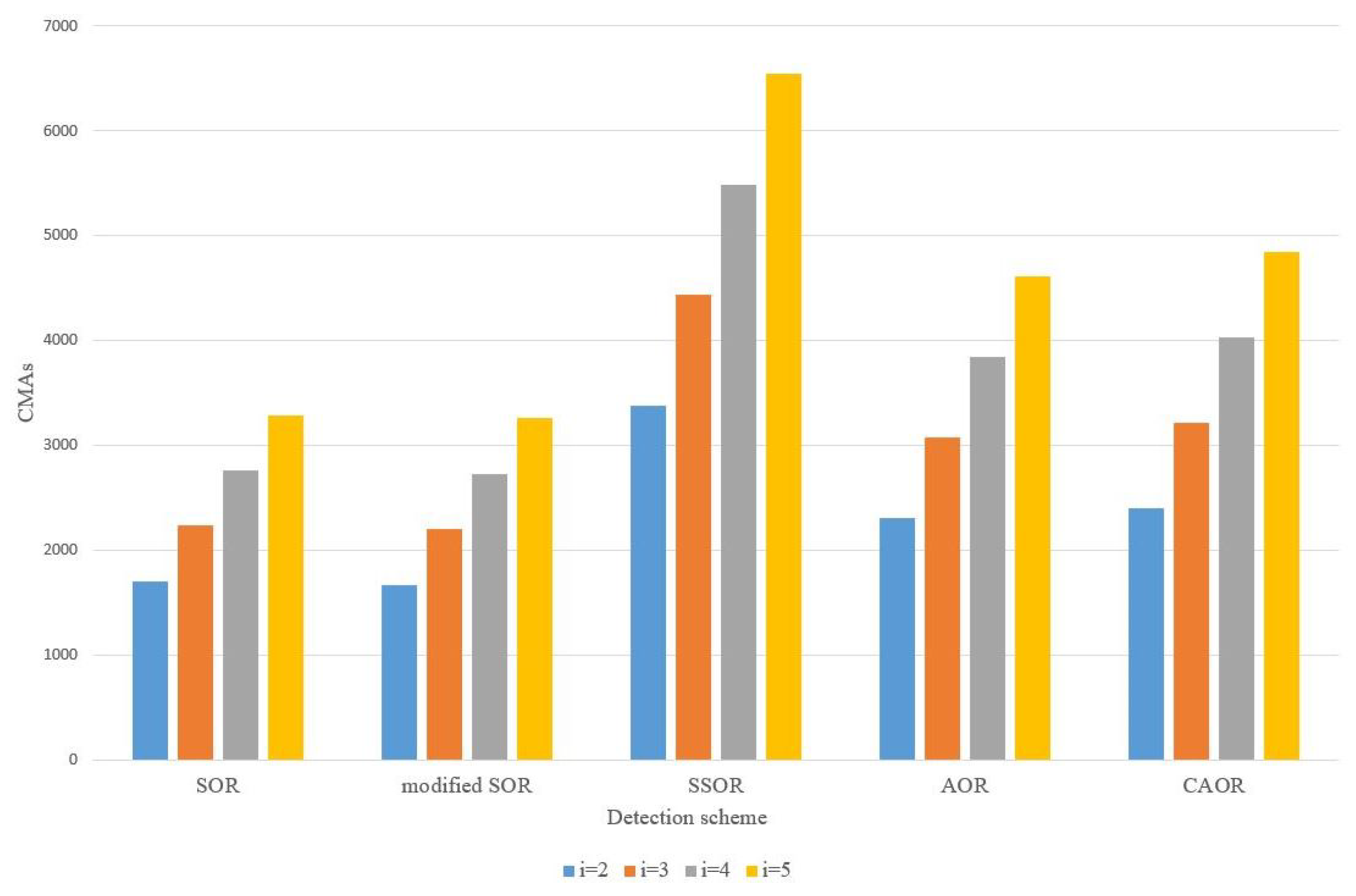
4.2. Computational Complexity Analysis

In this subsection, we evaluate the proposed detectors in terms of the computational complexity based on the number of complex multiplications required compared with other representative counterparts [27,28,29,30]. As in

Table 6. Computational complexity of different detection schemes.

Detection Scheme	Complex Multiplications and Additions (CMAs)
SOR	$\frac{1}{2}(5N_T^2+N_T)+i(2N_T^2+N_T)$
modified SOR	$\frac{1}{2}(5N_T^2-3N_T)+i(2N_T^2+N_T)$
SSOR	$5N_T^2-N_T+2i(2N_T^2+N_T)$
AOR	$3N_T^2+3i{N}_T^2$
CAOR	$3N_T^2+3i(N_T^2+N_T)$

, we give the computational complexity of different detection schemes, in which i and $N_T$ denote the number of iterations and the total number of user antennas, respectively. In addition, the inverse matrix of each iteration method requires $2N_T^2-N_T$ complex multiplications and additions (CMAs) [28]. We consider the CAOR iterative equation as follows:

$${\tilde{\mathbf{x}}}^{(k)}=M^{-1}·\frac{2{\mu }_k}{{\mu }_{(k-1)}\rho }·(N{\tilde{\mathbf{x}}}^{(k-1)}+\omega \mathbf{b})-\frac{{\mu }_k}{{\mu }_{(k-2)}}{\tilde{\mathbf{x}}}^{(k-2)},$$

(41)

in which $M^{-1}={(D+\gamma L)}^{-1}$ and $N=(1-\omega )D-(\omega -\gamma )L-\omega L^H$ require $2N_T^2-N_T$ CMAs and $N_T^2$ CMAs, respectively. Additionally, $\omega \mathbf{b}$ requires $N_T$ CMAs; as discussed above, we can obtain $3N_T^2$ CMAs, which is part of the CAOR’s computational complexity, as shown in Table 6. For the iteration part of CAOR, $M^{-1}·\frac{2{\mu }_k}{{\mu }_{(k-1)}\rho }·(N{\tilde{\mathbf{x}}}^{(k-1)}+\omega \mathbf{b})$ and $-\frac{{\mu }_k}{{\mu }_{(k-2)}}{\tilde{\mathbf{x}}}^{(k-2)}$ require $i(3N_T^2+N_T)$ CMAs and $2i{N}_T$ CMAs, respectively. Thus, the iteration part of the CAOR’s computational complexity requires $3i(N_T^2+N_T)$ CMAs altogether. Further, the numerical comparison of the complexity is shown in

Table 7. The numerical comparison of the complexity for different detection schemes with $N_T=16$.

Detection	CMAs	CMAs	CMAs	CMAs
Scheme	$\mathit{i}=2$	$\mathit{i}=3$	$\mathit{i}=4$	$\mathit{i}=5$
SOR	1704	2232	2760	3288
modified SOR	1672	2200	2728	3256
SSOR	3376	4432	5488	6544
AOR	2304	3072	3840	4608
CAOR	2400	3216	4032	4848

.

Regarding the complexity and performance factors, as shown in Figure 5, even though the BER performance of SSOR [29] is approximately $2.5\times {10}^{-3}$, which is also close to the conventional MMSE scheme, its complexity is approximately 37.8% higher than the CAOR method, which can be verified by the equation within Table 6. Meanwhile, we also know that the computational complexity of SSOR is the highest among all detectors, which is shown in Table 7.

For a more detailed discussion, we first consider four iterations in Figure 8; the CAOR method has improvements of 93% in BER compared with the conventional AOR. Meanwhile, the complexity only increases by 192 CMAs (increases by 5%). On the other hand, the CAOR method with $i=4$ only requires 4032 CMAs, which can achieve similar performance to the conventional AOR with $i=5$ requiring 4608 CMAs. Alongside this, when $N_R\times N_T=64\times 16$ and the iteration number is four, SSOR’s complexity and BER performance both are worse than AOR, not to mention compared with the CAOR method. The more complete numerical computational complexity in terms of iteration number for different detectors is shown in Table 7.

Secondly, to further observe the effect on BER and complexity when the number of antennas is increased, according to Figure 6 and Figure 10, as $N_R$ increases, the number of iterations required apparently gradually decreases. Furthermore, the BER performance and the computational complexity of CAOR decrease more than other detection methods.

Clearly, as shown in Figure 10, the BER performance of the proposed scheme only requires two iterations due to the sufficient number of antennas, which can achieve better BER performance than SOR, modified SOR, SSOR, and AOR. Meanwhile, as shown in Table 7, the complexity of CAOR at i = 2 and AOR at i = 3; they require 2400 CMAs and 3072 CMAs, respectively. The BER performance of CAOR and AOR is equal to $9.26\times {10}^{-5}$ and $8.24\times {10}^{-5}$, respectively; they are very close to each other. In light of the above discussion, we can conclude that as the number of antennas increases, the number of iterations will decrease gradually, and thus it is conducive to reducing the CMAs.

Therefore, as a whole, the computational complexity of CAOR is actually lower than that of conventional AOR. To show the computational complexity of different detection schemes more clearly, we utilize a bar graph to depict them in Figure 11.

5. Conclusions

In this paper, a novel two-stage receiver combining Chebyshev acceleration and the AOR algorithm (CAOR) is proposed to improve the convergence rate and achieve remarkable BER performance in a small number of iterations. Numerical results demonstrate the performance comparison with the different detection methods, in which the performance of CAOR is the best among all other detection methods. Although this method raises the computational load slightly more than AOR, fortunately, this is acceptable since the hardware’s computation ability is growing nowadays. Moreover, it can achieve a similar performance as SSOR and AOR with fewer iterations. Hence, the computational complexity of the proposed method is actually lower than expected. To sum up, regarding the BER performance and complexity, our proposed scheme is beyond comparison.

In summary, the M-MIMO has the ability to promote BER performance significantly in the 5G OFDMA systems, and our proposed method can achieve an appropriate acceleration parameter $\gamma$ and relaxation parameter $\omega$ and has the best BER under moderate computational complexity, so it is very suitable to apply to the current and next-generation wireless systems.

References

1. Andrews, J.G.; Buzzi, S.; Choi, W.; Hanly, S.V.; Lozano, A.; Soong, A.C.; Zhang, J.C. What will 5G be? IEEE J. Sel. Areas Commun. 2014, 32, 1065–1082. [Google Scholar] [CrossRef]
2. Boccardi, F.; Heath, R.W., Jr.; Lozano, A.; Marzetta, T.L.; Popovski, P. Five Disruptive Technology Directions for 5G. IEEE Commun. Mag. 2014, 52, 74–80. [Google Scholar] [CrossRef] [Green Version]
3. Agiwal, M.; Roy, A.; Saxena, N. Next Generation 5G Wireless Networks: A Comprehensive Survey. IEEE Commun. Surv. Tutor. 2016, 18, 1617–1655. [Google Scholar] [CrossRef]
4. Al-Fuqaha, A.; Guizani, M.; Mohammadi, M.; Aledhari, M.; Ayyash, M. Internet of Things: A Survey on Enabling Technologies, Protocols, and Applications. IEEE Commun. Surv. Tutor. 2015, 17, 2347–2376. [Google Scholar] [CrossRef]
5. Nawara, D.; Kashef, R. IoT-based Recommendation Systems–An Overview. In Proceedings of the 2020 IEEE International IOT, Electronics and Mechatronics Conference (IEMTRONICS), Vancouver, BC, Canada, 9–12 September 2020; pp. 1–7. [Google Scholar]
6. Borkar, S.; Pande, H. Application of 5G Next Generation Network to Internet of Things. In Proceedings of the 2016 International Conference on Internet of Things and Applications (IOTA), Pune, India, 22–24 January 2016; pp. 443–447. [Google Scholar]
7. Cho, Y.S.; Kim, J.; Yang, W.Y.; Kang, C.G. MIMO-OFDM Wireless Communications with Matlab; John Wiley & Sons: Singapore, 2010. [Google Scholar]
8. Prasad, R. OFDM for Wireless Communications Systems; Artech: Norwood, MA, USA, 2004. [Google Scholar]
9. Gesbert, D.; Shafi, M.; Shiu, D.S.; Smith, P.J.; Naguib, A. From Theory to Practice: An Overview of MIMO Space-Time Coded Wireless Systems. IEEE J. Sel. Areas Commun. 2003, 21, 281–302. [Google Scholar] [CrossRef] [Green Version]
10. Paulraj, A.J.; Gore, D.A.; Nabar, R.U.; Bölcskei, H. An Overview of MIMO Communications—A Key to Gigabit Wireless. Proc. IEEE 2004, 92, 198–218. [Google Scholar] [CrossRef] [Green Version]
11. Di Renzo, M.; Haas, H.; Ghrayeb, A.; Sugiura, S.; Hanzo, L. Spatial modulation for generalized MIMO: Challenges, opportunities, and implementation. IEEE Trans. Veh. Technol. 2014, 57, 2228–2241. [Google Scholar] [CrossRef]
12. Stuber, G.L.; Barry, J.R.; McLaughlin, S.W.; Li, Y.G.; Ingram, M.A.; Pratt, T.G. Broadband MIMO-OFDM Wireless Communications. Proc. IEEE 2004, 92, 271–294. [Google Scholar] [CrossRef] [Green Version]
13. Hwang, T.; Yang, C.; Wu, G.; Li, S.; Li, G.Y. OFDM and Its Wireless Applications: A Survey. IEEE Trans. Veh. Technol. 2009, 58, 1673–1694. [Google Scholar] [CrossRef]
14. Lu, L.; Li, G.Y.; Swindlehurst, A.L.; Ashikhmin, A.; Zhang, R. An Overview of Massive MIMO: Benefits and Challenges. IEEE J. Sel. Top. Signal Process. 2014, 8, 742–758. [Google Scholar] [CrossRef]
15. Larsson, E.G.; Tufvesson, F.; Edfors, O.; Marzetta, T.L. Massive MIMO for Next Generation Wireless Systems. IEEE Commun. Mag. 2014, 52, 186–195. [Google Scholar] [CrossRef] [Green Version]
16. Zheng, K.; Zhao, L.; Mei, J.; Shao, B.; Xiang, W.; Hanzo, L. Survey of Large-Scale MIMO Systems. IEEE Commun. Surv. Tutor. 2015, 17, 1738–1760. [Google Scholar] [CrossRef] [Green Version]
17. Björnson, E.; Larsson, E.G.; Marzetta, T.L. Massive MIMO: Ten Myths and One Critical Question. IEEE Commun. Mag. 2016, 54, 114–123. [Google Scholar] [CrossRef] [Green Version]
18. Marzetta, T.L. Noncooperative Cellular Wireless with Unlimited Numbers of Base Station Antennas. IEEE J. Sel. Areas Commun. 2010, 9, 3590–3600. [Google Scholar] [CrossRef]
19. Hoydis, J.; ten Brink, S.; Debbah, M. Massive MIMO in the UL/DL of Cellular Networks: How Many Antennas Do We Need? IEEE J. Sel. Areas Commun. 2013, 31, 160–171. [Google Scholar] [CrossRef] [Green Version]
20. Rusek, F.; Persson, D.; Lau, B.K.; Larsson, E.G.; Marzetta, T.L.; Edfors, O.; Tufvesson, F. Scaling Up MIMO: Opportunities and Challenges with Very Large Arrays. IEEE Signal Process. Mag. 2013, 30, 40–60. [Google Scholar] [CrossRef] [Green Version]
21. Larsson, E.G. MIMO Detection Methods: How They Work [lecture notes]. IEEE Signal Process. Mag. 2009, 26, 91–95. [Google Scholar] [CrossRef] [Green Version]
22. Wu, M.; Yin, B.; Wang, G.; Dick, C.; Cavallaro, J.R.; Studer, C. Large-Scale MIMO Detection for 3GPP LTE: Algorithms and FPGA Implementations. IEEE J. Sel. Top. Signal Process. 2014, 8, 916–929. [Google Scholar] [CrossRef] [Green Version]
23. Yin, B.; Wu, M.; Studer, C.; Cavallaro, J.R.; Dick, C. Implementation Trade-Offs for Linear Detection in Large-Scale MIMO Systems. In Proceedings of the IEEE Acoustics, Speech and Signal Processing (ICASSP), Vancouver, BC, Canada, 26–31 May 2013; pp. 2679–2683. [Google Scholar]
24. Albreem, M.A.; Salah, W.; Kumar, A.; Alsharif, M.H.; Rambe, A.H.; Jusoh, M.; Uwaechia, A.N. Low Complexity Linear Detectors for Massive MIMO: A Comparative Study. IEEE Access 2021, 9, 45740–45753. [Google Scholar] [CrossRef]
25. Kong, B.Y.; Park, I.C. Low-Complexity Symbol Detection for Massive MIMO Uplink Based on Jacobi Method. In Proceedings of the IEEE Annual International Symposium on Personal, Indoor, and Mobile Radio Communications (PIMRC), Valencia, Spain, 4–8 September 2016; pp. 1–5. [Google Scholar]
26. Wu, Z.; Zhang, C.; Xue, Y.; Xu, S.; You, X. Efficient Architecture for Soft-Output Massive MIMO Detection with Gauss-Seidel Method. In Proceedings of the IEEE International Symposium on Circuits and Systems (ISCAS), Montreal, QC, Canada, 22–25 May 2016; pp. 1886–1889. [Google Scholar]
27. Gao, X.; Dai, L.; Hu, Y.; Wang, Z.; Wang, Z. Matrix Inversion-Less Signal Detection Using SOR Method for Uplink Large-Scale MIMO Systems. In Proceedings of the IEEE Global Communications Conference (GLOBECOM), Austin, TX, USA, 8–12 December 2014; pp. 3291–3295. [Google Scholar]
28. Yu, A.; Zhang, C.; Zhang, S.; You, X. Efficient SOR-Based Detection and Architecture for Large-Scale MIMO Uplink. In Proceedings of the 2016 IEEE Asia Pacific Conference on Circuits and Systems (APCCAS), Jeju, Korea, 25–28 October 2016; pp. 402–405. [Google Scholar]
29. Ning, J.; Lu, Z.; Xie, T.; Quan, J.; You, X. Low Complexity Signal Detector Based on SSOR Method for Massive MIMO Systems. In Proceedings of the 2015 IEEE International Symposium on Broadband Multimedia Systems and Broadcasting (BMSB), Ghent, Belgium, 17–19 June 2015; pp. 1–4. [Google Scholar]
30. Zhang, Z.; Dai, X.; Dong, Y.; Wang, X.; Liu, T. A Low-Complexity Signal Detection Utilizing AOR Iterative Method for Massive MIMO Systems. China Commun. 2017, 9, 269–278. [Google Scholar] [CrossRef]
31. Young, D.M. Iterative Solution of Large Linear Systems; Elsevier: Amsterdam, The Netherlands, 2014. [Google Scholar]
32. Morelli, M.; Kuo, C.-C.J.; Pun, M.-O. Synchronization Techniques for Orthogonal Frequency Division Multiple Access (OFDMA): A Tutorial Review. Proc. IEEE 2007, 95, 1394–1427. [Google Scholar] [CrossRef]
33. Ng, D.; Lo, E.; Schober, R. Energy-Efficient Resource Allocation in OFDMA Systems with Large Numbers of Base Station Antennas. IEEE Trans. Wirel. Commun. 2012, 11, 3292–3304. [Google Scholar] [CrossRef]
34. Coleri, S.; Ergen, M.; Puri, A.; Bahai, A. Channel Estimation Techniques Based On Pilot Arrangement in OFDM Systems. IEEE Trans. Broadcast. 2002, 48, 223–229. [Google Scholar] [CrossRef] [Green Version]
35. Van de Beek, J.; Edfors, O.; Sandell, M.; Wilson, S.K.; Borjesson, P.O. On Channel Estimation in OFDM Systems. In Proceedings of the IEEE 45th Vehicular Technology Conference, Chicago, IL, USA, 25–28 July 1995; pp. 815–819. [Google Scholar]
36. Hadjidimos, A. Successive overrelaxation (SOR) and related methods. Comput. Appl. Math. 2000, 123, 177–199. [Google Scholar] [CrossRef] [Green Version]
37. Hadjidimos, A. Accelerated Overrelaxation Method. Math. Comput. 1978, 32, 149–157. [Google Scholar] [CrossRef]
Figure 1. The block diagram of the proposed two-stage detection scheme.
Electronics 11 00092 g001
Figure 2. BER performance of CAOR method against γ with SNR = 40 dB, N R × N T = 64 × 16 , and number of iterations i = 4.
Electronics 11 00092 g002
Figure 3. BER performance of CAOR method against ω with SNR = 40 dB, N R × N T = 64 × 16 , and number of iterations i = 4.
Electronics 11 00092 g003
Figure 4. BER performance comparison for different detection schemes, N R × N T = 64 × 16 .
Electronics 11 00092 g004
Figure 5. BER performance comparison for different detection schemes, N R × N T = 128 × 16 .
Electronics 11 00092 g005
Figure 6. BER performance comparison for different detection schemes, N R × N T = 256 × 16 .
Electronics 11 00092 g006
Figure 7. BER vs. β for different detection schemes when i = 2 and SNR is 40 dB.
Electronics 11 00092 g007
Figure 8. BER performance vs. number of iterations with N R × N T = 64 × 16 and SNR = 50 dB.
Electronics 11 00092 g008
Figure 9. BER performance vs. number of iterations with N R × N T = 128 × 16 and SNR = 45 dB.
Electronics 11 00092 g009
Figure 10. BER performance vs. number of iterations with N R × N T = 256 × 16 and SNR = 40 dB.
Electronics 11 00092 g010
Figure 11. Computational complexity of different detection schemes with N T = 16 .
Electronics 11 00092 g011