Fast Motion Model of Road Vehicles with Artificial Neural Networks

Abstract

Nonlinear optimization-based motion planning algorithms have been successfully used for dynamically feasible trajectory planning of road vehicles. However, the main drawback of these methods is their significant computational effort and thus high runtime, which makes real-time application a complex problem. Addressing this field, this paper proposes an algorithm for fast simulation of road vehicle motion based on artificial neural networks that can be used in optimization-based trajectory planners. The neural networks are trained with supervised learning techniques to predict the future state of the vehicle based on its current state and driving inputs. Learning data is provided for a wide variety of randomly generated driving scenarios by simulation of a dynamic vehicle model. The realistic random driving maneuvers are created on the basis of piecewise linear travel velocity and road curvature profiles that are used for the planning of public roads. The trained neural networks are then used in a feedback loop with several variables being calculated by additional numerical integration to provide all the outputs of the original dynamic model. The presented model can be capable of short-term vehicle motion simulation with sufficient precision while having a considerably faster runtime than the original dynamic model.

1. Introduction

1.1. Literature Outlook

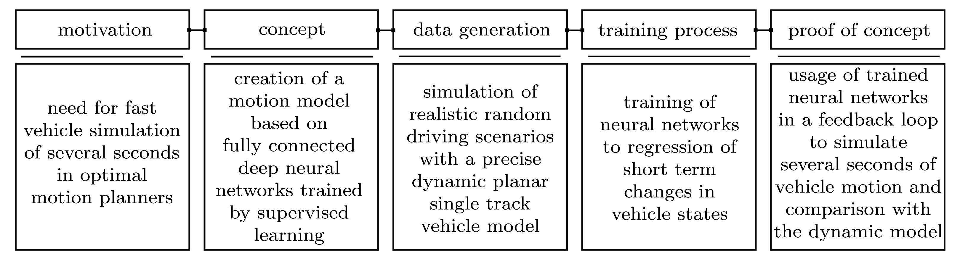
Automation of road transportation is expected to provide several benefits for society. Autonomous vehicles are expected to be more energy-efficient and environmentally friendly [1], while automated road traffic is predicted to improve average travel time significantly and traffic flow capacity [2], with the information provided by various sensors, communications and HD maps [3]. One of the most exciting research fields regarding autonomous driving is motion planning. Nonlinear optimization-based techniques have been used successfully to plan dynamically feasible trajectories for systems with nonholonomic dynamics. Optimization-based constrained trajectory generation algorithms are used for robot-assisted surgeries [4], machining equipment [5], and multi-purpose robots [6] as well as for road vehicles. One of the fundamental works on motion planning for wheeled vehicles is [7], where authors define an optimization framework suitable for driving a planetary robot on rough terrain. The winning team of the DARPA Urban Challenge at Carnegie Mellon University later used a similar nonlinear optimization-based trajectory planning and tracking algorithm [8]. In [9], the authors present a real-time fast and robust motion planning framework for urban conditions by combining a hybrid A*-based search with model predictive approaches to enable continuous re-planning based on current measurements. An optimization-based maneuver planning and tracking framework is proposed in [10] for low-speed and restricted-space environments using kinematic equations to describe the motion of cars, trucks, and semi-trailers. The authors of this paper propose a real-time trajectory planning algorithm in [11], where the dynamical feasibility of the motion is ensured by model-based simulation of the vehicle. The main difficulty in the case of all online optimization-based motion planning approaches is that the applied dynamical models have to be simulated numerous times as the cost and constraint functions need to be evaluated iteratively during the optimization loop. This means that considering an online optimization loop of approximately 100–200 ms, the available time for one vehicle simulation is in the range of 5 ms. Accordingly, there is an elementary need for fast and accurate short term vehicle simulation techniques in the field of optimal motion planning.

Numerous efficient simulation approaches have been developed for other time-critical applications such as computer graphics as well. In most cases, computer graphics functions require real-time performance for visualization, which means that the time available for the simulation of dynamic systems can often fall below even 1 ms. Position-Based Dynamics (PBD) directly computes the position-like dynamical quantities instead of time integration of equations of motions derived from Newton’s second law [12,13]. Subspace simulation methods are used to reduce the complexity of dynamic models by projecting the equations of motion into a reduced subspace with the help of, e.g., Principal Component Analysis (PCA) for a more efficient solution [14,15]. Data-driven physical simulations use data precomputed offline by accurate dynamic simulation techniques to approximate and/or accelerate online simulations. Artificial neural network-based data-driven models are an attractive opportunity for time-critical simulations because they enable faster run-times at the price of offline pre-calculations and higher memory usage [16,17]. Researchers at Ubisoft and McGill University are combining subspace simulation techniques with supervised learning in a computer graphics application where the computation time available for one object is in the range of 10–100 microseconds to simulate deformation effects, collisions of objects, and external forces [18].

Artificial neural networks are already used in vehicle simulation and control applications as well. In [19], authors are using artificial neural networks for modeling the main combustion metrics of diesel engines as an alternative for parameter tuning of dynamical models. Authors in [20] are simulating vertical tire and suspension dynamics while traversing road irregularities with recurrent neural networks. Another worthy example is [21], where deep feedforward networks are used to model and simulate a hovercraft. A robust neural network-based lateral control method is proposed in [22], which aims to resolve high-frequency oscillation issues of classical Sliding Mode Control (SMC) with the application of Radial Basis Function Neural Networks (RBFNN). Similarly, authors of [23] combine Model Predictive Control (MPC) with RBFNN to robustly handle the nonlinear characteristics of the steering system. A reinforcement-learning-based integrated planning and control method is proposed for automated parking applications in [24], which can simultaneously coordinate the longitudinal and lateral motions to park in a smaller parking space in one maneuver. Reinforcement learning is also used for high velocity lane change maneuvering in [25], where a Deep Deterministic Policy Gradient (DDPG) agent is utilized in an end-to-end method using lidar data. The authors of this paper are also actively researching this field. In [26], a hybrid motion planning approach is presented that unites classical optimization with neural networks for the more efficient solution of the planning problem. A reinforcement-learning-based lane keeping planning algorithm is developed in [27], where the machine learning agents are applied to support the Monte Carlo Tree Search (MCTS)-based planning in order to provide real-time performance.

As shown, artificial neural networks have been successfully utilized for physical simulations in numerous different research fields to enhance simulation speeds or replace physical models with many parameters.

1.2. Motivation

The motivations to create a neural network based vehicle model are twofold. Firstly, one can train the neural network based on real vehicle measurement data. This would enable us to perform simulations that are completely tailored to the vehicle in question, without having to worry about the correct parametrization of a dynamic model with a high degree of freedom. Secondly, the neural network can also be trained based on simulated vehicle motion data using a dynamic model of arbitrary complexity. The goal and expected benefit here is to decrease computational effort and thus runtime of the simulations using the neural-network-based model. Fast vehicle motion simulations of several (≤10) s are extremely useful for the application in online optimization-based motion planner algorithms as the evaluation of cost and constraint functions inside the optimization loop requires predicting the vehicle’s motion in case of numerous different values of the optimized variable [28]. This often means several hundreds of simulations that can be done faster with the neural-network-based model. The plausibility of the optimization results obtained this way can subsequently be supervised with a simulation of the original dynamic model. A single simulation does not cause runtime issues, even with a fairly complex vehicle model.

The contribution of this paper is accordingly a neural-network-based road vehicle model that is able to substitute a classic nonlinear single-track dynamical model in short-term simulations, while being faster as well. The paper is organized as follows. First, Section 2 describes the original dynamic model of the vehicle. In Section 3, a random trajectory planning algorithm is shown that is used to generate learning data for the neural-network-based approach. Then, in Section 4, the neural-network-based vehicle model is presented in details. Simulation results and performance evaluation of the proposed algorithm are described in Section 5. The limitation and potential issues of this study are later discussed in Section 6. Finally, Section 7 contains concluding remarks and proposals for future research directions.

Figure 1 shows the progress of the presented research from our motivation to create a neural-network-based vehicle model to the proof of concept of the developed method.

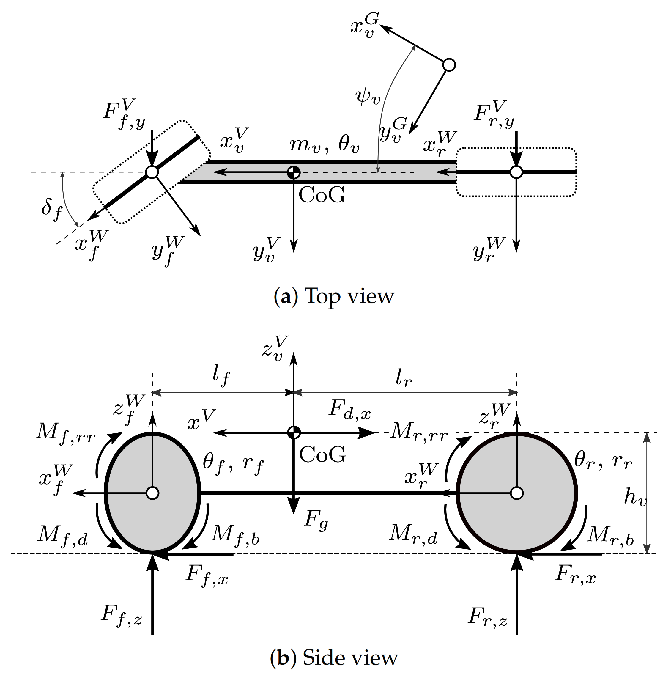
2. Nonlinear Single Track Vehicle Model

In this section, the applied planar nonlinear single-track vehicle model will be presented in detail. Planar single-track models are widely used for vehicle simulations and model-based calculations because they can offer sufficient precision in most driving scenarios on public roads while having a moderate complexity. Authors use the presented model in optimization-based motion planning algorithms as well, which makes it a good candidate for the proof of concept of the proposed neural-network-based model. The presented model combines literature sources, focusing on either chassis or wheel dynamics by using a sophisticated dynamic wheel slip model to increase the precision of simulations and also extends them with practical considerations that enable a stable and efficient numerical solution. Standard notations used for the equations of the vehicle model are the following. Superscripts differentiate between the same quantities in different coordinate systems. Specifically, superscript G stands for global inertial coordinate system NWU (North West Up), superscript V denotes the rotating vehicle-fixed coordinate system, and superscript W is applied for quantities in wheel-fixed coordinate systems. As numerous equations have to be calculated both for front and rear wheels the same way, subscript $[f/r]$ is used many times to indicate that by selecting subscript f or r for the whole equation, respectively, the equations are shown for both wheels. Similarly, subscript $[x/y]$ is used when the calculations for longitudinal and lateral directions are equivalent.

2.1. Model Components

The presented nonlinear single-track vehicle model shown in Figure 2 is a planar rigid multi-body model. The term single-track means that the wheels at the front and rear axles are substituted by one wheel per axle. Single-track models are widely used for vehicle simulations and model-based calculations because they can offer sufficient precision in most driving scenarios while having a moderate complexity [29]. The multi-body model consists of 3 bodies; the vehicle chassis and the two wheels, which are connected rigidly. Our model is planar, which means that vertical translation and roll and pitch movements are completely neglected. The vehicle is subject to Earth’s gravitational acceleration g. The center of gravity location of the vehicle is considered to be constant.

Wheel slips are modeled dynamically with respect to the elasticity of the tires. The longitudinal and lateral tire forces are nonlinear functions of corresponding wheel slips with respect to their simultaneous presence (superposition of forces is considered). Aligning torques on the wheels due to lateral slip is neglected. The vehicle has front-wheel steering, and the dynamics of steering actuation are considered. Driving inputs consist of total driving and braking torques as well as the steering wheel angle.

The presented model can precisely simulate driving scenarios even with high accelerations at the limit of adhesion and stability while having a moderate computational effort compared to full four-wheel 3D models. However, it cannot consider vertical dynamic effects such as road unevenness or load transitions due to road slope. Furthermore, scenarios where all four wheels’ friction conditions play an important role, such as $\mu$-split cases—where the left and right side of the vehicle meets with different road surface—cannot be simulated.

2.2. Dynamics of the Chassis

The vehicle chassis is a rigid planar body with three degrees of freedom: longitudinal and lateral positions $x_v^G$ and $y_v^G$ and yaw angle ${\psi }_v$ in the global inertial coordinate system. The chassis’ equations of motion represent the principles of conservation of linear and angular momentum (Newton’s second law) and are expressed in the inertial global coordinate system as follows:

$$\begin{array}{cc}\hfill {\ddot{x}}_v^G& =\frac{1}{m_v}(F_{fa,x}^G+F_{ra,x}^G+F_{d,x}^G),\hfill \end{array}$$

(1)

$$\begin{array}{cc}\hfill {\ddot{y}}_v^G& =\frac{1}{m_v}(F_{fa,y}^G+F_{ra,y}^G+F_{d,y}^G),\hfill \end{array}$$

(2)

$$\begin{array}{cc}\hfill {\ddot{\psi }}_v& =\frac{1}{{\theta }_{v,z}}(l_{v,f}{F}_{fa,y}^V-l_{v,r}{F}_{ra,y}^V),\hfill \end{array}$$

(3)

where $m_v$ is the total mass of the vehicle, ${\theta }_{v,z}$ is its the moment of inertia about the vertical axis, and horizontal distances of vehicle center of gravity to front and rear axles are noted by $l_{v,[f/r]}$. Aerodynamic drag forces are first calculated in the vehicle-fixed coordinate system as

$$\begin{array}{cc}\hfill F_{d,x}^V& =\frac{1}{2}{c}_{v,d}{A}_{v,f}{\rho }_A{\dot{x}}_v^V\sqrt[]{{\left({\dot{x}}_v^V\right)}^2+{\left({\dot{y}}_v^V\right)}^2},\hfill \end{array}$$

(4)

$$\begin{array}{cc}\hfill F_{d,y}^V& =\frac{1}{2}{c}_{v,d}{A}_{v,f}{\rho }_A{\dot{y}}_v^V\sqrt[]{{\left({\dot{x}}_v^V\right)}^2+{\left({\dot{y}}_v^V\right)}^2},\hfill \end{array}$$

(5)

where $A_{v,f}$ is the frontal area and $c_{v,d}$ is the aerodynamic drag coefficient of the vehicle, while ${\rho }_A$ is the density of air [29]. The conversion of arbitrary dynamic quantity ${\gamma }_{[x/y]}$ in the rotating vehicle-fixed coordinate system to the global inertial one is done by

$$\begin{array}{cc}\hfill {\gamma }_x^G& =+cos\left({\psi }_v\right){\gamma }_x^V-sin\left({\psi }_v\right){\gamma }_y^V,\hfill \end{array}$$

(6)

$$\begin{array}{cc}\hfill {\gamma }_y^G& =+sin\left({\psi }_v\right){\gamma }_x^V+cos\left({\psi }_v\right){\gamma }_y^V.\hfill \end{array}$$

(7)

Similarly, the conversion from the global inertial coordinate system to the vehicle-fixed is

$$\begin{array}{cc}\hfill {\gamma }_x^V& =+cos\left({\psi }_v\right){\gamma }_x^G+sin\left({\psi }_v\right){\gamma }_y^G,\hfill \end{array}$$

(8)

$$\begin{array}{cc}\hfill {\gamma }_y^V& =-sin\left({\psi }_v\right){\gamma }_x^G+cos\left({\psi }_v\right){\gamma }_y^G.\hfill \end{array}$$

(9)

Accordingly, the aerodynamic drag forces calculated in Equations (4) and (5) are transformed to the inertial global coordinate system by Equations (6) and (7). As the model is planar (vertical movements are neglected), one can calculate the tire loads based on equilibrium of forces and moments in the vertical plane as

$$\begin{array}{c}\hfill F_{f,z}^V=\frac{m_{v}g{l}_{v,r}-h_v(F_{fa,x}^V+F_{ra,x}^V)}{l_{v,f}+l_{v,r}},\end{array}$$

(10)

$$\begin{array}{c}\hfill F_{r,z}^V=\frac{m_{v}g{l}_{v,f}+h_v(F_{fa,x}^V+F_{ra,x}^V)}{l_{v,f}+l_{v,r}},\end{array}$$

(11)

where $h_v$ is the center of gravity height of the vehicle. Driving and braking torques are distributed ideally according to the load transfer above, which means the resulting longitudinal slips shall be equalized by torques calculated as

$$\begin{array}{c}\hfill M_{[f/r],d}=\frac{c_{[f/r],M}}{c_{f,M}+c_{r,M}}{M}_d,\end{array}$$

(12)

$$\begin{array}{c}\hfill M_{[f/r],b}=\frac{c_{[f/r],M}}{c_{f,M}+c_{r,M}}{M}_b,\end{array}$$

(13)

with $c_{[f/r],M}=r_{[f/r]}{F}_{[f/r],z}^V$ where $M_d$ and $M_b$ are the non-negative driving and braking torque inputsb [30]. Calculation of the applied longitudinal and lateral tire forces $F_{[f/r]a,[x/y]}^{(·)}$ is detailed in Section 2.3.

We are often interested in the inertial accelerations not only in the global coordinate system, but in the vehicle-fixed one as well. To calculate their values ${\ddot{x}}_{v,I}^V$, ${\ddot{y}}_{v,I}^V$, from global accelerations ${\ddot{x}}_v^G$, ${\ddot{y}}_v^G$ we can use Equations (8) and (9). Please note that these accelerations are not equal to the translational accelerations in the vehicle-fixed system, because the vehicle is rotating.

2.3. Dynamics of the Wheels

The front and rear virtual wheels have a single degree of freedom: rotation about their own axes ${\rho }_{[f/r]}$. Longitudinal and lateral wheel slips $s_{[f/r],[x/y]}$ are calculated according to a dynamic model considering elasticity of the tires. The dynamic equations of the wheels are as follows:

$$\begin{array}{cc}\hfill {\ddot{\rho }}_{[f/r]}=& \frac{1}{{\theta }_{[f/r]}}\left(M_{[f/r],d}-r_{[f/r]}{F}_{[f/r]a,x}^W-M_{[f/r],ba}-M_{[f/r],rra}\right),\hfill \end{array}$$

(14)

$$\begin{array}{cc}\hfill {\dot{s}}_{[f/r],x}=& \frac{1}{l_{[f/r]a,x}}\left(v_{[f/r],r}-{\dot{x}}_{[f/r]}^W-\left|{\dot{x}}_{[f/r]}^W\right|s_{[f/r],x}\right),\hfill \end{array}$$

(15)

$$\begin{array}{cc}\hfill {\dot{s}}_{[f/r],y}=& \frac{1}{l_{[f/r]a,y}}\left(-{\dot{y}}_{[f/r]}^W-\left|{\dot{x}}_{[f/r]}^W\right|s_{[f/r],y}\right),\hfill \end{array}$$

(16)

where $r_{[f/r]}$ are the radii and ${\theta }_{[f/r]}$ are the moments of inertia of the wheels. The rolling velocities of the wheels are calculated as

$$v_{[f/r],r}=r_{[f/r]}{\dot{\rho }}_{[f/r]}.$$

(17)

The braking torque shall only be applied to the wheels if they are moving, calculated as

$$M_{[f/r],ba}=\left\{\begin{array}{cc}\mathrm{sign}\left(v_{[f/r],r}\right)M_{[f/r],b},\hfill & \mathrm{if}{v}_{[f/r],r}>v_{ba}\hfill \\ \mathrm{sign}\left(v_{[f/r],r}\right)M_{[f/r],b}\frac{1}{2}\left(1-cos\left(\pi \frac{\left|v_{[f/r],r}\right|}{v_{ba}}\right)\right),\hfill & \mathrm{if}{v}_{[f/r],r}\le v_{ba}\hfill \end{array}\right.$$

(18)

where $v_{ba}=v_{ba,0}+k_{v_{ba}}\left|M_{[f/r],b}\right|$ is the rolling velocity at which braking torque damping should disappear. With this approach, the value of applied braking torque is gradually built down as the wheel stops, so that it can reach an oscillation-free standstill state. Rolling resistance torques are first calculated as

$$M_{[f/r],rr}=\mathrm{sign}\left(v_{[f/r],r}\right)F_{[f/r],z}^W{r}_f[A_{rr}+B_{rr}\left|v_{[f/r],r}\right|+C_{rr}{\left(v_{[f/r],r}\right)}^2],$$

(19)

where $A_{rr}$, $B_{rr}$, and $C_{rr}$ are parameters [31]. Tire loads are the same in the vehicle-fixed and in the wheel-fixed coordinate systems $F_{[f/r],z}^W=F_{[f/r],z}^V$ due to the common vertical axis. Then, a damping technique similar to one applied to the acting braking torque is used to eliminate discontinuity at point $v_{[f/r],r}$ = 0, so that the acting rolling resistance torques are built up gradually while the wheels are starting to move as follows:

$$M_{[f/r],rra}=\left\{\begin{array}{cc}{M}_{[f/r],rr},\hfill & \mathrm{if}{v}_{[f/r],r}>v_{rra}\hfill \\ M_{[f/r],rr}\frac{1}{2}\left(1-cos\left(\pi \frac{\left|v_{[f/r],r}\right|}{v_{rra}}\right)\right),\hfill & \mathrm{if}{v}_{[f/r],r}\le v_{rra}\hfill \end{array}\right.$$

(20)

where $v_{rra}$ is the rolling velocity at which rolling resistance torque should be fully applied.

Tire forces are generally calculated as a function of slip according to the Magic Formula in the coordinate systems of corresponding wheels as

$$\begin{array}{cc}\hfill F_{[f/r],[x,y]}^W\left(s\right)=& {\mu }_{[f/r]}{F}_{[f/r],z}^W{D}_{[f/r],[x,y]}sin\{C_{[f/r],[x,y]}arctan(B_{[f/r],[x,y]}s-\hfill \\ \hfill & E[B_{[f/r],[x,y]}s-arctan\left(B_{[f/r],[x,y]}s\right)]\left)\right\},\hfill \end{array}$$

(21)

where ${\mu }_{[f/r]}$ is the static coefficient of friction and $D_{[f/r],[x,y]}$ are the maximum factors, $C_{[f/r],[x,y]}$ are the shape factors, $B_{[f/r],[x,y]}$ are the stiffness factors, and $E_{[f/r],[x,y]}$ are the curvature factors of the tire model [32]. To improve the low-speed behavior of the model especially when starting from or braking until standstill, the tire forces are calculated based on damped slip values [32], which are evaluated as

$$\begin{array}{cc}\hfill s_{[f/r]d,x}& =s_{[f/r],x}+\frac{k_{[f/r]d,x}}{K_{[f/r],x}}\left(v_{[f/r],r}-{\dot{x}}_{[f/r]}^W\right),\hfill \end{array}$$

(22)

$$\begin{array}{cc}\hfill s_{[f/r]d,y}& =s_{[f/r],y},\hfill \end{array}$$

(23)

with slip stiffness being

$$K_{[f/r],[x,y]}={\mu }_{[f/r]}{F}_{[f/r],z}^W{D}_{[f/r],[x,y]}{C}_{[f/r],[x,y]}{B}_{[f/r],[x,y]}.$$

(24)

The factor of slip damping is calculated with the usual cosine transition as

$$k_{[f/r]d,x}=\left\{\begin{array}{cc}0,\hfill & \mathrm{if}{\dot{x}}_f^W>v_{sd}\hfill \\ k_{[f/r],x}\frac{1}{2}\left(1+cos\left(\pi \frac{|{\dot{x}}_f^W|}{v_{sd}}\right)\right),\hfill & \mathrm{if}{\dot{x}}_f^W\le v_{sd}\hfill \end{array}\right.,$$

(25)

where $v_{sd}$ is the rolling velocity at which slip damping should switch off and $k_{[f/r],x}$ is the initial maximal factor of damping [32]. In case of pure longitudinal or lateral slip conditions, the tire forces are calculated simply by

$$F_{[f/r]n,[x,y]}^W=F_{[f/r],[x,y]}^W\left(s_{[f/r]d,[x/y]}\right).$$

(26)

In case of the mutual presence of longitudinal and lateral wheel slips tire forces are calculated with respect to their superposition by the friction ellipse method, given as

$$\begin{array}{cc}\hfill F_{[f/r]c,x}^W& =\mathrm{sign}\left(s_{[f/r]d,x}\right)\sqrt{\frac{{\left(F_{[f/r],x}^W\left(s_{[f/r]d,c}\right)F_{[f/r],y}^W\left(s_{[f/r]d,c}\right)\right)}^2}{{\left(F_{[f/r],y}^W\left(s_{[f/r]d,c}\right)\right)}^2+{\left(\frac{s_{[f/r]d,y}}{s_{[f/r]d,x}}{F}_{[f/r],x}^W\left(s_{[f/r]d,c}\right)\right)}^2}},\hfill \end{array}$$

(27)

$$\begin{array}{cc}\hfill F_{[f/r]c,y}^W& =\mathrm{sign}\left(s_{[f/r]d,y}\right)\sqrt{\frac{{\left(F_{[f/r],x}^W\left(s_{[f/r]d,c}\right)F_{[f/r],y}^W\left(s_{[f/r]d,c}\right)\right)}^2}{{\left(F_{[f/r],x}^W\left(s_{[f/r]d,c}\right)\right)}^2+{\left(\frac{s_{[f/r]d,x}}{s_{[f/r]d,y}}{F}_{[f/r],y}^W\left(s_{[f/r]d,c}\right)\right)}^2}}.\hfill \end{array}$$

(28)

with $s_{[f/r]d,c}=\sqrt{{\left(s_{[f/r]d,x}\right)}^2+{\left(s_{[f/r]d,x}\right)}^2}$ being the combined slip value. Finally, the acting tire forces are given by

$$F_{[f/r]a,[x/y]}^W=\left\{\begin{array}{cc}{F}_{[f/r]c,[x/y]}^W\hfill & \mathrm{if}{s}_{[f/r]d,[x,y]}>s_{da},\hfill \\ F_{[f/r]n,[x/y]}^W\hfill & \mathrm{if}{s}_{[f/r]d,[x,y]}\le s_{da},\hfill \end{array}\right.$$

(29)

where $s_{da}$ is the minimal value of wheel slips where superposition of forces shall be considered. This limit is important for the numerical calculations, as Equations (27) and (28) are singular at zero slip values. The acting tire forces of the front wheel given in its own coordinate system $F_{fa,[x/y]}^W$ can be transformed to the values in the vehicle-fixed frame $F_{fa,[x/y]}^V$ by substituting the yaw angle ${\psi }_v$ with steering angle ${\delta }_f$ in Equations (6) and (7). Since the vehicle has front wheel steering only, conversion for the rear wheels is not necessary as $F_{fa,[x/y]}^V=F_{fa,[x/y]}^W$. Further conversions from forces in the vehicle-fixed coordinate system $F_{[f/r]a,[x/y]}^V$ to the ones in the global inertial coordinate system $F_{[f/r]a,[x/y]}^G$ can be performed directly according to Equations (6) and (7).

To be able to evaluate the dynamic equations of the wheel, slip-dependent acting relaxation lengths of tires have to be calculated as

$$l_{[f/r]a,[x/y]}=max\left(l_{[f/r],[x/y]}\left(1-\frac{K_{[f/r],[x,y]}}{3D_{[f/r],[x,y]}}\left|s_{[f/r],[x,y]}\right|\right),l_{[f/r]m,[x/y]}\right),$$

(30)

where $l_{[f/r],[x/y]}$ and $l_{[f/r]m,[x/y]}$ are the relaxation lengths at standstill and at wheel spin or lock, respectively [32]. Furthermore, the velocities of wheel center points are needed in wheel-fixed coordinate systems. To obtain these, the velocities of the vehicle center of gravity in the global inertial coordinate system ${\dot{x}}_v^G$${\dot{y}}_v^G$ are first converted to the vehicle-fixed coordinate system ${\dot{x}}_v^V$${\dot{x}}_v^V$ with Equations (8) and (9). Then, wheel center point velocities are calculated as

$$\begin{array}{cc}\hfill {\dot{x}}_{[f/r]}^V& ={\dot{x}}_v^V,\hfill \end{array}$$

(31)

$$\begin{array}{cc}\hfill {\dot{y}}_f^V& ={\dot{y}}_v^V+l_{v,f}{\dot{\psi }}_v,\hfill \end{array}$$

(32)

$$\begin{array}{cc}\hfill {\dot{y}}_r^V& ={\dot{y}}_v^V-l_{v,r}{\dot{\psi }}_v.\hfill \end{array}$$

(33)

The wheel center point velocities finally have to be transformed to wheel-fixed coordinate systems. For the rear wheel, no real transformation is necessary as ${\dot{x}}_r^W={\dot{x}}_r^V$ and ${\dot{y}}_r^W={\dot{y}}_r^V$. As the front wheel is steered, Equations (8) and (9) can be used with the substitution of yaw angle ${\psi }_v$ with steering angle ${\delta }_f$ to get the values ${\dot{x}}_f^W$ and ${\dot{y}}_f^W$.

2.4. Steering Actuation

The vehicle model uses a simple first-order transfer function to consider the steering actuator. The steering dynamics are given by

$${\dot{\delta }}_f=\frac{k_s}{T_s}{\delta }_{sw}-\frac{1}{T_s}\delta ,$$

(34)

where ${\delta }_{sw}$ is the steering wheel angle input, $k_s$ is the steering ratio, and $T_s$ is the settling time of the steering mechanism. The trajectory tracking behavior of the vehicle is much more realistic, even with this very simple actuation model, than with the direct application of steering angles calculated by the tracking controllers.

2.5. Closed Loop Control

In order to follow a selected reference trajectory, we need tracking controllers to drive the presented vehicle model with control inputs—driving and braking torques and steering wheel angle. Longitudinal speed tracking control is performed by a state feedback LQR (Linear Quadratic Regulator) controller according to

$$M_{db}=-K_{v_1}{\dot{x}}_v^V-K_{v_2}{z}_v$$

(35)

where $K_{v_1}$ and $K_{v_2}$ are gain values and $z_v$ is the integral of velocity tracking error. The longitudinal controller computes a signed torque value which is then transformed to the non-negative driving inputs as

$$\begin{array}{c}\hfill M_d=max(M_{db},0),\end{array}$$

(36)

$$\begin{array}{c}\hfill M_b=|min(M_{db},0).|\end{array}$$

(37)

Path tracking is realized by a Stanley controller. This is a nonlinear feedback control that ensures asymptotic tracking of the reference path. According to the control law, the wheel level steering angle of the front axle is calculated as

$${\delta }_f=e_{\psi }+arctan(K_{st}\frac{e_{lat}}{{\dot{x}}_v^V}),$$

(38)

where $e_{\psi }$ is the yaw angle offset between the path and the vehicle, $e_{lat}$ is the lateral distance of the front axle center-point from the path, and $K_{st}$ is a tunable gain parameter [33]. The reference point for tracking error calculation is the closest point of the path curve to the center of the front axle.

2.6. Simulation of Model

The motion of the presented dynamic nonlinear single-track vehicle model must be calculated numerically by an Ordinary Differential Equation (ODE) solver with an appropriate time resolution. As a solver, we recommend second (Heun) or fourth-order (RK4) explicit Rungke–Kutta methods as they provide stable and fast computations. For reproducibility and convenient manageability of simulation output, a fixed step-size is used. Due to the wheels’ relatively fast and complex dynamics (especially in drive-off or brake-still scenarios), a relatively small step size $\mathrm{\Delta }{t}_v$ around 1 ms is required.

3. Random Trajectory Planning

Overall, the presented vehicle dynamics model has 15 states and five inputs, which have to be provided to the state equation to calculate state derivatives. With this number of variables, training sample generation by parameter sweeping is impossible. Considering only ten values for each input, the number of samples would reach 1.024 × 10¹³, which is very difficult to handle. Instead of the parameter sweeping, learning data are generated based on simulated scenarios. When defining the driving maneuvers, our goal is to create a wide variety of dynamic situations. Regarding longitudinal dynamics, sections with intensive acceleration and braking and smaller variations around a constant traveling velocity are necessary. Considering lateral dynamics, mild curves, as well as sharp turns, are essential to reach an extensive range of lateral acceleration. Combinations of curves with acceleration and braking are also desirable. Definition of these simulation maneuvers manually would be, on the one hand, a massive effort. On the other hand, it would probably also not provide the required diversity. Thus, a randomized motion planning approach is applied to generate the reference data for vehicle dynamics simulations.

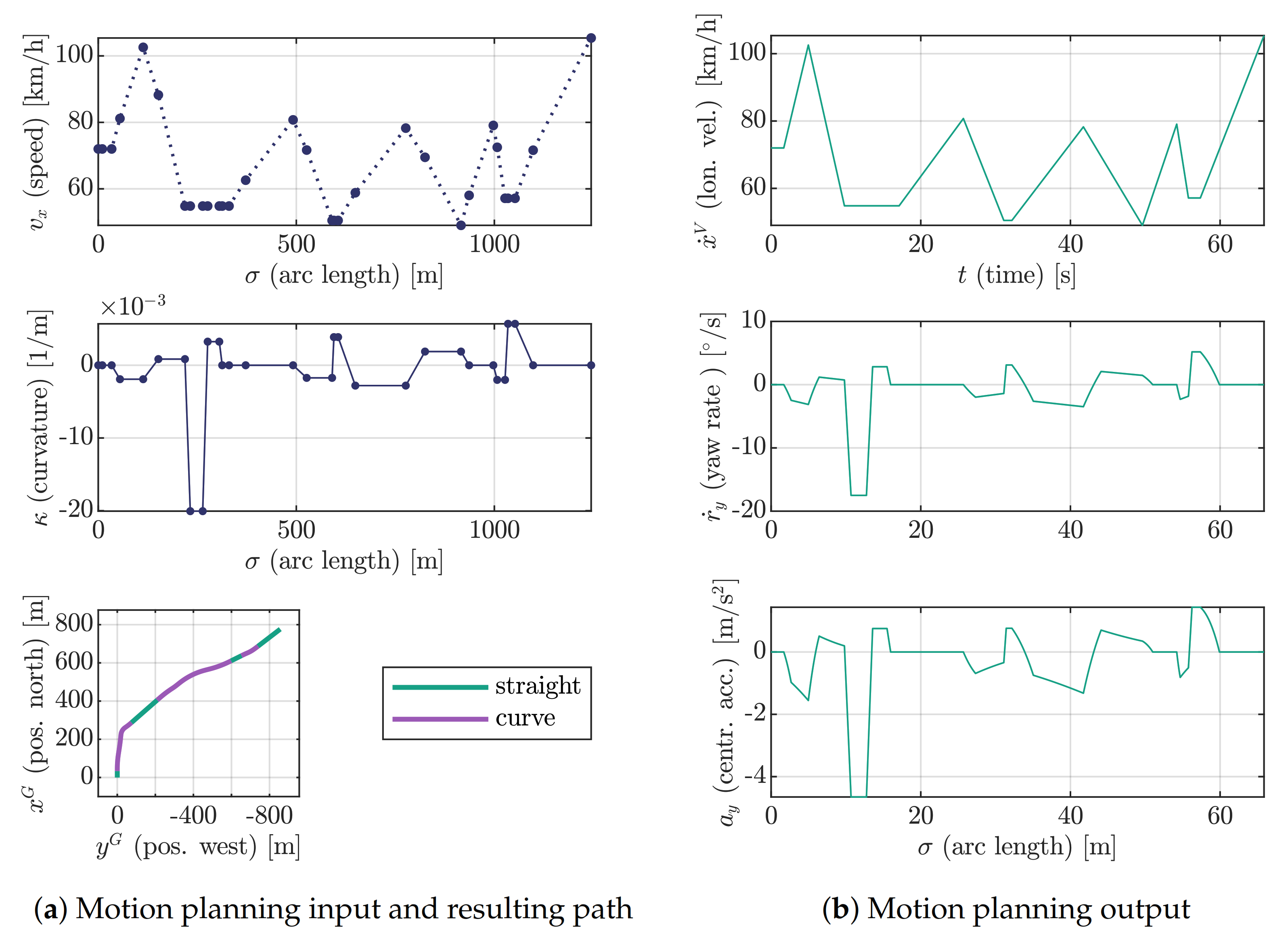
3.1. Motion Planning Based on Piecewise Linear Curvature and Travel Velocity Functions

The idea of path planning based on a piecewise linear curvature function comes from the real world, as horizontal geometry (alignment) of public roads in most cases consists of straight segments and circular arcs, connected by clothoid curves for a smooth transition [34]. While straight segments have zero curvature, and circular arcs have a constant curvature, the clothoid’s curvature is changing linearly with the arc length. Thus, road geometries in question can be defined by assigning a piecewise linear curvature profile as a function of the arc length along the path. Naturally, continuous derivative profiles could also be used, but their implementation would increase the complexity of the algorithm without giving a real benefit for the current application [35]. To get a driving trajectory, we also have to specify the traveling speed of the vehicle. This can be done simply and sufficiently by defining a piecewise linear speed profile as a function of time. Naturally, the curvature and speed profiles must be connected to provide a feasible trajectory—e.g., we have to slow down before high-curvature (low radius) sections.

Accordingly, the input of the trajectory planner is

$$X_p={\left[\begin{array}{ccc}{\sigma }_p^i& {\kappa }_p^i& {\dot{x}}_p^i\end{array}\right]}^T,i=1\dots N_p^i,$$

(39)

where ${\sigma }_p^i$ are the arc length, ${\kappa }_p^i$ are the curvature, and ${\dot{x}}_p^i$ are the traveling velocity knot points of the curvature and velocity profiles. The meaning of the input parametrization is that at arc length ${\sigma }_p^i$, the curvature of the path shall be ${\kappa }_p^i$ and the travel velocity shall be ${\dot{x}}_p^i$. Figure 3a (in blue) shows the input of the planning.

The time needed to travel along each path section can be calculated by

$$\mathrm{\Delta }{t}_p^i=\frac{\mathrm{\Delta }{\sigma }_p^i}{{\stackrel{\sim }{\dot{x}}}_p^i},$$

(40)

where $\mathrm{\Delta }{\sigma }_p^i={\sigma }_p^{i+1}-{\sigma }_p^i$ and ${\tilde{\dot{x}}}_p^i=\frac{{\dot{x}}_p^i+{\dot{x}}_p^{i+1}}{2}$ for $i=1\dots N_p^i-1$. The travel time at each knot point is then

$$t_p^{i+1}=\sum _1^i\mathrm{\Delta }{t}_p^i,$$

(41)

for $i=1\dots N_p^i-1$ with $t_1=0$. The constant longitudinal acceleration along each path section is given by

$${\ddot{x}}_p^i=\frac{\mathrm{\Delta }{\dot{x}}_p^i}{\mathrm{\Delta }{t}_p^i},$$

(42)

where $\mathrm{\Delta }{\dot{x}}_p^i={\dot{x}}_p^{i+1}-{\dot{x}}_p^i$ for $i=1\dots N_p^i-1$. For any arc length such that ${\sigma }_p\in [{\sigma }_p^i,{\sigma }_p^{i+1}]$ the travel time can be expressed as

$$t_p=\left\{\begin{array}{cc}\frac{\sigma -{\sigma }_p^i}{{\dot{x}}_p^i}+t_p^i\hfill & \mathrm{if}{\ddot{x}}_p^i=0,\hfill \\ \frac{-{\dot{x}}_p^i+\sqrt{{\left({\dot{x}}_p^i\right)}^2+2{\ddot{x}}_p^i(\sigma -{\sigma }_p^i)}}{{\ddot{x}}_p^i}+t_p^i\hfill & \mathrm{if}{\ddot{x}}_p^i\ne 0,\hfill \end{array}\right.$$

(43)

Based on the time information, travel velocity is calculated as

$${\dot{x}}_p={\dot{x}}_p^i+{\ddot{x}}_p^i(t_p-t_p^i).$$

(44)

By obtaining curvature with a simple interpolation

$${\kappa }_p={\kappa }_p^i+\frac{{\kappa }_p^{i+1}-{\kappa }_p^i}{{\sigma }_p^{i+1}-{\sigma }_p^i}{\sigma }_p,$$

(45)

yaw rate and centripetal acceleration are

$$\begin{array}{cc}\hfill {\dot{\psi }}_p& ={\dot{x}}_p{\kappa }_p,\hfill \end{array}$$

(46)

$$\begin{array}{cc}\hfill {\ddot{y}}_p& ={\dot{x}}_p{\dot{\psi }}_p.\hfill \end{array}$$

(47)

To be able to evaluate path coordinates, yaw (heading) angle is first calculated as

$${\psi }_p={\psi }_{p,0}+{\int }_0^{{\sigma }_p}{\dot{\psi }}_p,$$

(48)

where ${\psi }_{p,0}$ initial yaw angle is assumed for every trajectory. Then, longitudinal path coordinates can be calculated as

$$x_p=x_{p,0}+{\int }_0^{{\sigma }_p}cos\left({\psi }_p\right)ds,$$

(49)

and lateral path coordinates are evaluated as

$$y_p=y_{p,0}+{\int }_0^{{\sigma }_p}sin\left({\psi }_p\right)ds,$$

(50)

with the assumptions of $x_{p,0}=0$ and $y_{p,0}=0$. In practice Equations (40)–(42) are first calculated for each input knot points. Then, the total arc length domain is split with equidistant steps as

$${\sigma }_p^j=j{\sigma }_{p,s},j=0\dots N_p^j$$

(51)

where ${\sigma }_{p,s}$ (0.1 m) is a suitable step size and $N_p^j=\lceil \frac{{\sigma }_p^{N_p^i}}{{\sigma }_{p,s}}\rceil$. Equations (43)–(50) are then numerically calculated for the resulting arc length series. The output of the planner accordingly is

$$Y_p={\left[\begin{array}{cccc}{x}_p^j& y_p^j& {\psi }_p^j& {\dot{\psi }}_p^j,\end{array}\right]}^T,j=0\dots N_p^j,$$

(52)

and contains a series of path coordinates as well as yaw angle and yaw rate values along the trajectory that can be used as reference for vehicle dynamics control. The outputs of the trajectory planner can be seen on Figure 3b.

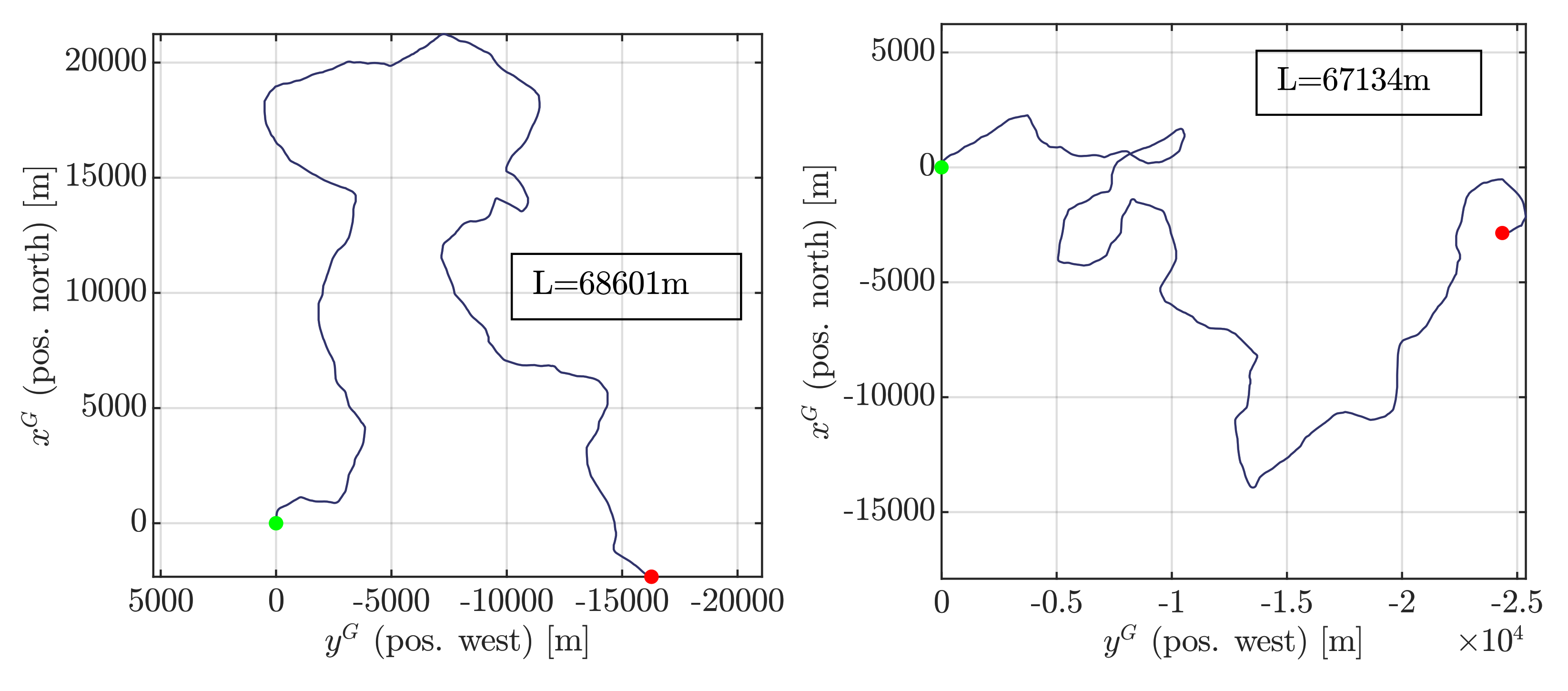
3.2. Random Planning

It is evident that we cannot just specify any input to the trajectory planner described in Section 3.1 to get a feasible trajectory. The calculations in the planner are solely geometric and are assuming that the traveling object is precisely following the given path and velocity. This means that the random trajectory planning must be constrained to provide a feasible reference to the vehicle simulation. The number of road sections $N_r$ (500) is chosen in advance (this means that number of profile knot points $N_p^i$ will be 501). The planning is carried out as follows.

•  The knot points ${\dot{x}}_p^i$ of the traveling velocity profile are chosen randomly between allowed lower ${\dot{x}}_{p,min}$ (10 m/s) and upper ${\dot{x}}_{p,max}$ (30 m/s) limits.
•  Minimal allowed radii are calculated for each section based on maximal allowed lateral acceleration ${\ddot{y}}_{p,max}$ (5 m/s²).

  $$r_{p,min}^i=\frac{{\left({\dot{x}}_p^i\right)}^2}{{\ddot{y}}_{p,max}}$$

  (53)
•  Radii $r_p^i$ of each section are chosen randomly in such a way that the values are between $r_{p,min}^i$ and $m_{r_{min}}{r}_{p,min}^i$. The factor $m_{r_{min}}$ (10) is a planning parameter.
•  Lengths $\mathrm{\Delta }{\sigma }_p^i$ of each section are chosen randomly in such a way that the values are between $p_{c_{min}}2\pi r_p^i$ and $p_{c_{max}}2\pi r_p^i$. The factors $p_{c_{min}}$ (0.1) and $p_{c_{max}}$ (0.2) are planning parameters.
•  Curvature values ${\kappa }_p^i=\frac{1}{r_p^i}$ are calculated, and half of them are inverted to provide left and right turns with equal probability.
•  A $p_s$ (0.35) proportion of the curvature values ${\kappa }_p^i$ is nulled out to provide straight segments in a way that neighboring straight segments are not allowed.
•  Transitions are calculated between each of the previous sections in such way that the proportion of their lengths to the segments lengths $p_t$ (0.4) is given.
•  Arc length knot points ${\sigma }_p^i$ are calculated by a cumulative sum of segment lengths $\mathrm{\Delta }{\sigma }_p^i$.
•  The curvature and travel velocity profile calculated in 1–8 is then provided to the planner described in Section 3.1 to get the random reference trajectory.

Example trajectories designed with the algorithm detailed in this section are shown in Figure 4.

4. Neural Network Based Vehicle Model

In this section, the developed neural-network-based vehicle model will be presented in detail. Our main goal with the presented algorithm is to provide quick neural-network-based vehicle simulations of maximally about 10 s, which can be obtained faster than the original dynamic model’s solution to use them in the online optimization loop of motion planner algorithms. First, the input–output structure, as well as the method of learning sample generation, is explained. Then, the architecture of used neural networks as well as the training process is shown. Last, the algorithm for vehicle motion simulation based on the trained neural networks is presented. For the modeling and training of artificial neural networks, we use the Python programming language and its packages tensorflow, keras and scikit-learn. The training is performed on a desktop computer with an Intel^® Core™ i5-7600 CPU, 32 GB of RAM, 500 GB of NVME SSD storage, and an NVIDIA^® GeForce GTX 1050 Ti GPU.

4.1. Input–Output Concept

The first important aspect of artificial-neural-network-based vehicle modeling is the input–output structure of the model. On the one hand, the artificial neural network could be used to estimate the equations of motion of the vehicle Equations (1)–(3), (14)–(16). With this approach, the output of the neural network consists of the same translational and angular accelerations that the original dynamic equations provide and thus must still be integrated the same way with an ODE solver and 1ms time step. As explored in earlier stages of the research, this approach has two significant disadvantages. As described in Section 1.2, the main goal of the neural-network-based model would be to decrease run-time of motion predictions. Firstly, the computation time of recalling the neural network should be less than the computation time of the original state equation, which strongly restricts the number of neurons usable in the network. Secondly, the estimation errors of the neural network are amplified by the ODE solver, causing the solution to diverge quickly. Due to the mentioned drawbacks, this approach is not presented in the paper.

On the other hand, direct estimation of the solution of the equations of motion of the vehicle is also possible. The aim here is to predict the vehicle’s state at time $t+\mathrm{\Delta }{t}_{nv}$ based on its state and input at time t, namely, to provide the solution of the ODEs for a time span of multiple 1 ms steps. Four different input–output variants were examined for this concept in the research, which are noted with V0, V1, V2, and V3, respectively. The input vector of the neural network consists of the inputs and a subset of state variables of the dynamic model at a given time t and is represented as

$$\begin{array}{ccc}\hfill X_{nv}^{V0,V1}\left(t\right)=\left[\begin{array}{c}{M}_{db}\left(t\right)\\ {\delta }_{sw}\left(t\right)\\ {\dot{x}}_v^V\left(t\right)\\ {\dot{y}}_v^V\left(t\right)\\ {\dot{\psi }}_v\left(t\right)\\ {\dot{\rho }}_f\left(t\right)\\ s_{f,x}\left(t\right)\\ s_{f,y}\left(t\right)\\ {\dot{\rho }}_r\left(t\right)\\ s_{r,x}\left(t\right)\\ s_{r,y}\left(t\right)\\ {\delta }_f\left(t\right)\end{array}\right],& \hfill & \hfill X_{nv}^{V2,V3}\left(t\right)=\left[\begin{array}{c}{M}_{db}\left(t\right)\\ {\delta }_{sw}\left(t\right)\\ {\psi }_v\left(t\right)\\ {\dot{x}}_v^V\left(t\right)\\ {\dot{y}}_v^V\left(t\right)\\ {\dot{\psi }}_v\left(t\right)\\ {\dot{\rho }}_f\left(t\right)\\ s_{f,x}\left(t\right)\\ s_{f,y}\left(t\right)\\ {\dot{\rho }}_r\left(t\right)\\ s_{r,x}\left(t\right)\\ s_{r,y}\left(t\right)\\ {\delta }_f\left(t\right)\end{array}\right].\end{array}$$

(54)

The only difference in the input vectors of different variants is that yaw angle ${\psi }_v\left(t\right)$ is additionally provided for the V2–3 networks. The output vector of the neural network consists of the changes of a subset of vehicle state variables as time reaches $t+\mathrm{\Delta }{t}_{nv}$, calculated as

$$\mathrm{\Delta }\xi \left(t\right)=\xi (t+\mathrm{\Delta }{t}_{nv})-\xi \left(t\right)$$

(55)

for a general state variable $\xi$, and is represented as

$$\begin{array}{ccccc}\hfill Y_{nv}^{V0}\left(t\right)=\left[\begin{array}{c}\mathrm{\Delta }{\dot{x}}_v^V\left(t\right)\\ \mathrm{\Delta }{\dot{y}}_v^V\left(t\right)\\ \mathrm{\Delta }{\dot{\psi }}_v\left(t\right)\\ \mathrm{\Delta }{\dot{\rho }}_f\left(t\right)\\ \mathrm{\Delta }{s}_{f,x}\left(t\right)\\ \mathrm{\Delta }{s}_{f,y}\left(t\right)\\ \mathrm{\Delta }{\dot{\rho }}_r\left(t\right)\\ \mathrm{\Delta }{s}_{r,x}\left(t\right)\\ \mathrm{\Delta }{s}_{r,y}\left(t\right)\\ \mathrm{\Delta }{\delta }_f\left(t\right)\end{array}\right],& \hfill & \hfill Y_{nv}^{V1.V2}\left(t\right)=\left[\begin{array}{c}\mathrm{\Delta }{\psi }_v\left(t\right)\\ \mathrm{\Delta }{\dot{x}}_v^V\left(t\right)\\ \mathrm{\Delta }{\dot{y}}_v^V\left(t\right)\\ \mathrm{\Delta }{\dot{\psi }}_v\left(t\right)\\ \mathrm{\Delta }{\dot{\rho }}_f\left(t\right)\\ \mathrm{\Delta }{s}_{f,x}\left(t\right)\\ \mathrm{\Delta }{s}_{f,y}\left(t\right)\\ \mathrm{\Delta }{\dot{\rho }}_r\left(t\right)\\ \mathrm{\Delta }{s}_{r,x}\left(t\right)\\ \mathrm{\Delta }{s}_{r,y}\left(t\right)\\ \mathrm{\Delta }{\delta }_f\left(t\right)\end{array}\right],& \hfill & \hfill Y_{nv}^{V3}\left(t\right)=\left[\begin{array}{c}\mathrm{\Delta }{x}_v^G\left(t\right)\\ \mathrm{\Delta }{y}_v^G\left(t\right)\\ \mathrm{\Delta }{\psi }_v\left(t\right)\\ \mathrm{\Delta }{\dot{x}}_v^V\left(t\right)\\ \mathrm{\Delta }{\dot{y}}_v^V\left(t\right)\\ \mathrm{\Delta }{\dot{\psi }}_v\left(t\right)\\ \mathrm{\Delta }{\dot{\rho }}_f\left(t\right)\\ \mathrm{\Delta }{s}_{f,x}\left(t\right)\\ \mathrm{\Delta }{s}_{f,y}\left(t\right)\\ \mathrm{\Delta }{\dot{\rho }}_r\left(t\right)\\ \mathrm{\Delta }{s}_{r,x}\left(t\right)\\ \mathrm{\Delta }{s}_{r,y}\left(t\right)\\ \mathrm{\Delta }{\delta }_f\left(t\right)\end{array}\right].\end{array}$$

(56)

The difference in the output vectors of different variants is that networks V1–3 directly estimate the heading angle difference $\mathrm{\Delta }{\psi }_v$, and network V4 directly estimatwa the changes in position $\mathrm{\Delta }{x}_v^G$ and $\mathrm{\Delta }{y}_v^G$ as well.

4.2. Learning Sample Generation

As the first step of the learning sample generation, random reference trajectories are generated by the motion planner described in Section 3. For current work, an equivalent amount of 10 h (∼680 km) driving was generated for training and another 4 h (∼270 km) for testing purposes, which means a 70–30% train-test split, approximately. Then, vehicle simulation was performed with the model described in Section 2 with a sample time of $\mathrm{\Delta }{t}_v=$1 ms. In order to provide the same amount of left and right turns to the learning process, data augmentation was used by mirroring (inverting the lateral motion components of) the simulated trajectories. Accordingly, an equivalent of 28 h of driving data were generated in total.

For the next step, the prediction time $\mathrm{\Delta }{t}_{nv}$ of the neural-network-based model has to be decided. On the one hand, the bigger this value is, the faster the motion prediction with the network will be. On the other hand, as the model is intended to be used in a motion planner algorithm, a certain resolution is necessary for reliable collision avoidance calculations. From the feasible set of prediction time values of 5, 10, 20, and 50 ms, $\mathrm{\Delta }{t}_{nv}=$10 ms was chosen as it provides a sufficient trade-off between run-time and resolution. The complete matrices of training input and output samples are then

$$\begin{array}{cc}\hfill I_{nv}^{tr}& ={\left[\begin{array}{ccccc}{X}_{nv}\left(0\right)& X_{nv}(\mathrm{\Delta }{t}_v)& X_{nv}(2\mathrm{\Delta }{t}_v)& \dots & X_{nv}((N_v^{tr}-1)\mathrm{\Delta }{t}_v-\mathrm{\Delta }{t}_{nv})\end{array}\right]}^T,\hfill \end{array}$$

(57)

$$\begin{array}{cc}\hfill O_{nv}^{tr}& ={\left[\begin{array}{ccccc}{Y}_{nv}\left(0\right)& Y_{nv}(\mathrm{\Delta }{t}_v)& Y_{nv}(2\mathrm{\Delta }{t}_v)& \dots & Y_{nv}((N_v^{tr}-1)\mathrm{\Delta }{t}_v-\mathrm{\Delta }{t}_{nv})\end{array}\right]}^T,\hfill \end{array}$$

(58)

where $N_v^{tr}$ is the total number of training vehicle simulation samples. Testing input $I_{nv}^{tt}$ and output $O_{nv}^{tt}$ samples are generated in the same way from the corresponding vehicle simulation samples. Maximum absolute values are calculated for each input and output variables separately for scaling as

$$\begin{array}{cc}\hfill c_{X_{nv}}& =\underset{t}{max}{X}_{nv}\left(t\right),\hfill \end{array}$$

(59)

$$\begin{array}{cc}\hfill c_{Y_{nv}}& =\underset{t}{max}{Y}_{nv}\left(t\right),\hfill \end{array}$$

(60)

commonly for training and testing samples. Both the input and output samples are then scaled in each variable (along each column) with these scales so that they only contain values in range of [−1, 1]. From the 28 h of driving data, approximately 70 million training samples as well as 28 million test samples were generated.

Since vehicle simulations are written in C++ for better performance and data preparation is mainly done in MATLAB, learning data must be written into files to be able to use them in Python for the training. Due to a large number of learning data (more than 16 GB), samples do not all fit into computer memory at once. For efficiency, learning input and output matrices $I_{nv}^{tr}$ and $I_{nv}^{tt}$ as well as $O_{nv}^{tr}$ and $O_{nv}^{tt}$ are written into multiple binary files in a column major order with one binary buffer containing 1024 batches of 8196 samples. The scaling vectors $c_{X_{nv}}$ and $c_{Y_{nv}}$ are also written to column major binary files for uniform data handling. Training metadata (number of inputs, outputs, samples, batch size, buffer size, variable names) are written to a JSON (JavaScript Object Notation) file for convenience.

To efficiently provide the learning data from the binary buffers, an own generator algorithm is necessary, which reads in the files only once per training epoch in a subsequent order. To achieve this, shuffling of learning data must be switched off in keras’ Model.fit method so that the training algorithm asks for the samples in increasing order. By knowing the number of samples per binary file from the metadata, it is easy to decide if a new file must be loaded. The generator algorithm also takes care of the shuffling of samples per buffer file by creating random indices for samples.

4.3. Neural Network Architecture

The estimation of vehicle simulation output is a regression task. For this, fully connected feed-forward deep neural networks are used with three or four intermediate layers and 256 neurons in total. Trying networks with a total neuron count of 96, 128, and 384 shows that with fewer neurons, the fitting results are much worse, and with more neurons, the slight improvement in performance is not worth the increased computational effort. For each I/O variant V1–4, four different networks are trained with layouts shown in

Table 1. Neural network layouts.

Name	Layout
n256l3v1	[64, 128, 64]
n256l3v2	[32, 192, 32]
n256l4v1	[32, 96, 96, 32]
n256l4v2	[64, 128, 128, 64]

.

As an activation function, ReLU (Rectified Linear Unit) is applied for each layer except for the output layer using linear activation. Experimenting with other activation functions such as sigmoid, hyperbolic tangent, or SELU (Scaled Exponential Linear Unit) shows worse performance without exception.

4.4. Training Process

To compute the loss during the training, a custom weighted mean squared error function is used as

$$L_{nv}=\frac{1}{n_{Y_{nv}}}\sum _{i=1}^{n_{Y_{nv}}}{w}_{L_{nv}}^i{(Y_{nn}^i-{\widehat{Y}}_{nn}^i)}^2,$$

(61)

where $n_{Y_{nv}}$ is the number of elements of the output vector, $w_{L_{nv}}^i$ are custom weighting factors for each output variable, and prediction of neural network is denoted with ${\widehat{Y}}_{nn}$. The rationale behind using this weighted loss instead of the standard mean squared error loss is that the precision of velocity and position predictions is more important than, for instance, the slip variables.

The Adam optimizer waschosen, which is a stochastic gradient descent method that is based on adaptive estimation of first-order and second-order moments. Adam optimizer is generally recommended as “computationally efficient, has little memory requirement, invariant to diagonal rescaling of gradients, and is well suited for problems that are large in terms of data/parameters” [36]. Learning rate multipliers 0.1, 0.3, 0.5, and 1 are applied to the default value of learning rate 0.001 to search for optimal training results.

Learning progress of the neural networks reaching the smallest final loss is shown in Figure 5. On the left side, the best results are shown for each topology in Table 1. On the right side, the results for the best network overall are shown. The number of training epochs is chosen as 100 for a balance between training time and performance. Batch size is selected for 8196 samples. The training time of a network with a single set of parameters is approximately 1 h due to the learning samples not fitting into memory at once. With the selected number of training epochs, no overfitting is visible. An increased number of 140 training epochs shows no real performance improvement.

4.5. Motion Prediction in Feedback Loop

As explained in Section 4.1, at a certain time t, the neural network is capable of predicting the changes in vehicle state variables and thus the new state of the vehicle at a $\mathrm{\Delta }{t}_{nv}$ = 10 ms later time. This is a nice result, but the final aim of the research is to predict several seconds of vehicle motion as stated in Section 1.2. To enable this, an iterative calculation is necessary, where the neural network acts in a feedback loop. In this loop, the estimation of the new state at $t+\mathrm{\Delta }{t}_{nv}$ is fed back to the input of the neural network to predict the new state at $t+2\mathrm{\Delta }{t}_{nv}$, and this goes on for the whole period of the simulation. Depending on the I/O variant, it may also be necessary to compute the yaw angle ${\psi }_{nv}$ (for V0) as well as the position coordinates $x_{nv}^G$ and $y_{nv}^G$ (for V0–2) with numerical integration, as they are not estimated directly by the neural network. State derivatives of the original dynamic model also need to be calculated numerically for all network variants. Initially, total simulation time $t_{nv}$ is split into equidistant steps of $\mathrm{\Delta }{t}_{nv}$, denoting the resulting time series as $t_{nv}^j$ with $j=0\dots \lceil \frac{t_{nv}}{\mathrm{\Delta }{t}_{nv}}\rceil$. The initial value of input vector $X_{nv}\left(t_{nv}^0\right)$ is assembled from initial values of vehicle inputs and states. Then, simulation happens in the following loop:

•  Input vector $X_{nv}\left(t_{nv}^j\right)$ is applied to the neural network to compute output $Y_{nv}\left(t_{nv}^j\right)$. In practice, input and output vectors must be scaled with the scaling vectors in Equations (59) and (60), but this is not reflected to in the equations for the sake of simplicity.
•  Vehicle state variables for which estimations $\mathrm{\Delta }\xi \left(t_{nv}^j\right)$ are available in the neural network output $Y_{nv}\left(t_{nv}^j\right)$ are calculated by

  $$\xi \left(t_{nv}^{j+1}\right)=\xi \left(t_{nv}^j\right)+\mathrm{\Delta }\xi \left(t_{nv}^j\right)$$

  (62)

  for general state $\xi$.
•  For variant V0, yaw angle is calculated by numerical integration as

  $${\psi }_{nv}\left(t_{nv}^{j+1}\right)=\frac{\mathrm{\Delta }{\dot{\psi }}_{nv}\left(t_{nv}^j\right)+\mathrm{\Delta }{\dot{\psi }}_{nv}\left(t_{nv}^{j+1}\right)}{2}\mathrm{\Delta }{t}_{nv}.$$

  (63)
•  For variants V0–2, position coordinates are calculated by numerical integration as

  $$\begin{array}{cc}\hfill x_{nv}^G\left(t_{nv}^{j+1}\right)& =\frac{{\dot{x}}_{nv}^G\left(t_{nv}^j\right)+{\dot{x}}_{nv}^G\left(t_{nv}^{j+1}\right)}{2}\mathrm{\Delta }{t}_{nv},\hfill \end{array}$$

  (64)

  $$\begin{array}{cc}\hfill y_{nv}^G\left(t_{nv}^{j+1}\right)& =\frac{{\dot{y}}_{nv}^G\left(t_{nv}^j\right)+{\dot{y}}_{nv}^G\left(t_{nv}^{j+1}\right)}{2}\mathrm{\Delta }{t}_{nv},\hfill \end{array}$$

  (65)

  where velocities ${\dot{x}}_{nv}^G$ and ${\dot{y}}_{nv}^G$ are calculated from ${\dot{x}}_{nv}^V$ and ${\dot{y}}_{nv}^V$ by a rotation with −${\psi }_{nv}$.
•  Vehicle state derivative variables for which estimations $\mathrm{\Delta }\xi \left(t_{nv}^j\right)$ are available in the neural network output $Y_{nv}\left(t_{nv}^j\right)$ are estimated directly with differences

  $$\dot{\xi }\left(t_{nv}^{j+1}\right)\simeq \frac{\mathrm{\Delta }\xi \left(t_{nv}^j\right)}{\mathrm{\Delta }{t}_{nv}}$$

  (66)

  for general state $\xi$.
•  Inertial accelerations in momentaneous vehicle frame are evaluated as

  $$\begin{array}{cc}\hfill {\ddot{x}}_{nv,I}^V\left(t_{nv}^{j+1}\right)& =\frac{\mathrm{\Delta }{\dot{x}}_{nv}^V\left(t_{nv}^j\right)}{\mathrm{\Delta }{t}_{nv}}-{\dot{y}}_{nv}^V\left(t_{nv}^j\right){\dot{\psi }}_{nv}\left(t_{nv}^j\right),\hfill \end{array}$$

  (67)

  $$\begin{array}{cc}\hfill {\ddot{y}}_{nv,I}^V\left(t_{nv}^{j+1}\right)& =\frac{\mathrm{\Delta }{\dot{y}}_{nv}^V\left(t_{nv}^j\right)}{\mathrm{\Delta }{t}_{nv}}+{\dot{x}}_{nv}^V\left(t_{nv}^j\right){\dot{\psi }}_{nv}\left(t_{nv}^j\right),\hfill \end{array}$$

  (68)

  to take the rotating frame of reference into account.
•  Input vector of next step, $X_{nv}\left(t_{nv}^{j+1}\right)$ is assembled from vehicle inputs and results of Equation (62).
•  Steps 1–7 are repeated until simulation is finished.

Accordingly, our neural-network-based vehicle model consists of the network itself, which can predict the state of the vehicle for 10 ms, and the feedback loop algorithm described above, which uses the network to provide simulation results for several seconds. The presented approach can provide all the outputs that are available when using the original dynamical model. It is important to mention that the results coming from the presented simulation loop differ from the output of the original dynamic model even when assuming that the neural network is providing a perfect regression fit. The reason for this difference is, on the one hand, that state variables in Equations (63)–(65) are calculated with the forward Euler method (compared to the more sophisticated ODE solution of the dynamic model) and also on a sub-sampled dataset. On the other hand, state-derivative variables in Equation (66) are estimated with numeric differences (instead of the dynamic equations) and on a sub-sampled dataset as well.

5. Simulation Results

This section presents the simulation results of the neural-network-based vehicle model described in Section 4. The evaluations and comparisons in this chapter were mainly made in MATLAB, which can utilize the trained neural networks from keras. First, an example of the regression fit of the standalone neural network is presented and analyzed. Then, a closed-loop vehicle motion simulation example is shown to give a picture of the performance of the proposed algorithm in terms of output signals. Finally, the performance of different variants is evaluated.

5.1. Regression Fit

Figure 6 shows the regression results of the trained neural network for a sequence of testing samples that are coming directly from the dynamic vehicle simulation without shuffling. The number of 10,000 samples is the equivalent of 10 s dynamic simulation with a sample rate of 1 ms. As the output of the neural network consists of the changes in states $\mathrm{\Delta }\xi \left(t\right)$, these values are proportional to the derivative values of the corresponding states $\dot{\xi }\left(t\right)$. Please note that all outputs are normalized to the range of [−1, 1]. Accordingly, the selected sequence of samples contains a scenario with considerable acceleration and braking as well as moderate steering and has an intermediate complexity from a dynamics point of view. The estimation of the neural network fits well to the output samples. The estimation error is, in all cases, more than one order of magnitude smaller than the estimated signal itself. Overall variables are shown, the maximal estimation error is 0.0727, and the mean estimation error is 0.0196.

Table 2. Regression fit error statistic of a typical trained neural network.

Variable	EMAX	MAE	Variable	EMAX	MAE
		$\times {\mathbf{10}}^{-\mathbf{2}}$			$\times {\mathbf{10}}^{-\mathbf{2}}$
$\mathrm{\Delta }{\dot{x}}_v^V\left(t\right)$	0.17043	0.08441	$\mathrm{\Delta }{s}_{f,x}\left(t\right)$	0.93073	0.09424
$\mathrm{\Delta }{\dot{y}}_v^V\left(t\right)$	0.16793	0.07394	$\mathrm{\Delta }{s}_{f,y}\left(t\right)$	0.16374	0.08827
$\mathrm{\Delta }{\dot{\psi }}_v\left(t\right)$	0.24512	0.08250	$\mathrm{\Delta }{s}_{r,x}\left(t\right)$	0.42943	0.08377
$\mathrm{\Delta }{\dot{\rho }}_f\left(t\right)$	0.82452	0.15126	$\mathrm{\Delta }{s}_{r,y}\left(t\right)$	0.13317	0.05913
$\mathrm{\Delta }{\dot{\rho }}_r\left(t\right)$	0.51242	0.14104	$\mathrm{\Delta }{\delta }_f\left(t\right)$	0.15871	0.04865

shows the typical values of estimation errors for a trained neural network for the most important output variables. The notation E_MAX stands for maximal absolute error, while MAE (Mean Absolute Error) is used conventionally. We can see the biggest estimation errors in the case of changes in wheel speeds and longitudinal slip values. This behavior is logical, since the piecewise linear travel velocity profile that is used for the input sample generation results in a square-shaped longitudinal acceleration (and wheel angular acceleration) signal with jumps (this can be seen in Figure 6 as well). Learning these jumps is complicated for the neural network. While E_MAX values are very high for these variables, they are only reached for a minimal number of samples. As MAE values show, average estimation error remains very small even in these cases. In comparison, changes in lateral slip values are much slower since the clothoid transition segments between the circular arcs and straight sections enable lateral tire forces (and wheel slips) to build up gradually. Accordingly, corresponding E_MAX values are much slower. In general, we can say that while the regression provided by the neural network is not perfect, it is sufficient to be used for short-term vehicle simulations presented in Section 5.2.

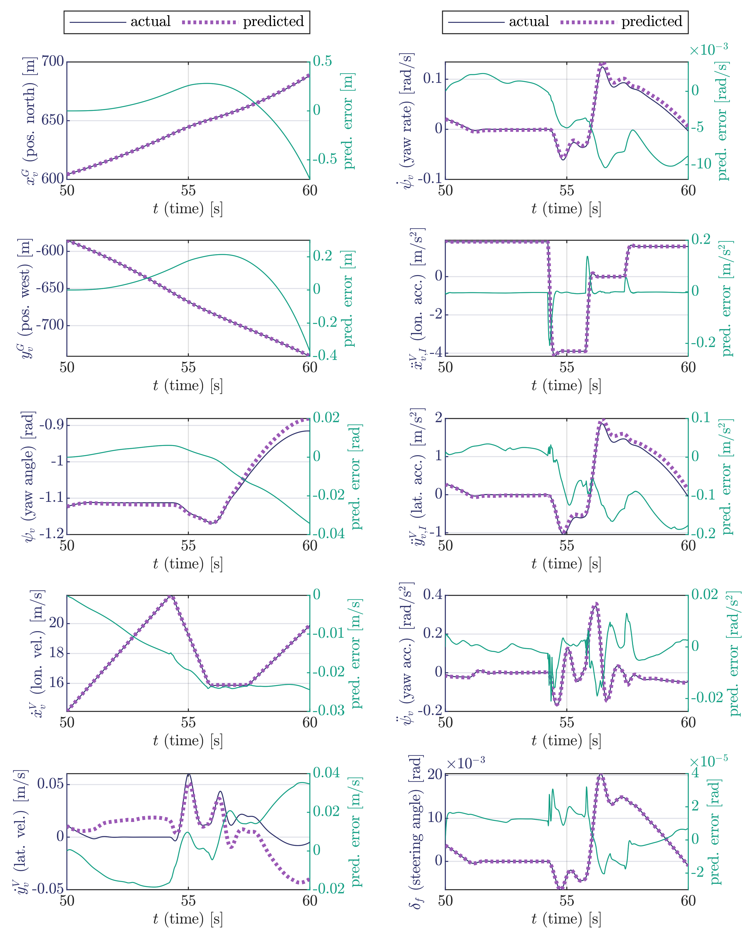
5.2. Prediction of Vehicle Motion

Figure 7 shows the performance of the neural network based vehicle motion simulation in the case of the most important state variables.

The selected scenario is a 10 s long part of the test dataset and has an average dynamical complexity with longitudinal acceleration reaching −4 m/s² and lateral acceleration exceeding 2 m/s². The output of the neural network based model is able to nicely reproduce the output of the original dynamic model. The maximum error of position estimation is below 60 cm, and the maximal yaw (heading) angle estimation error remains under 2${}^{\circ }$. Prediction error of longitudinal velocity does not exceed 0.03 m/s, while yaw rate prediction error is below 0.6${}^{\circ }$/s. Inertial accelerations are also calculated with a maximal error of 0.2 m/s². The biggest error can be observed in the case of lateral velocity, where the neural-network-based solution occasionally has a large offset of 0.05 m/s. However, the importance of this state variable from the motion planning point of view is not as high as that of the other ones listed above. The results show that with the application of appropriate safety boundaries applied to the position of the vehicle, the output of the neural-network-based model can be used for motion prediction in the online optimization loop of trajectory planner algorithms.

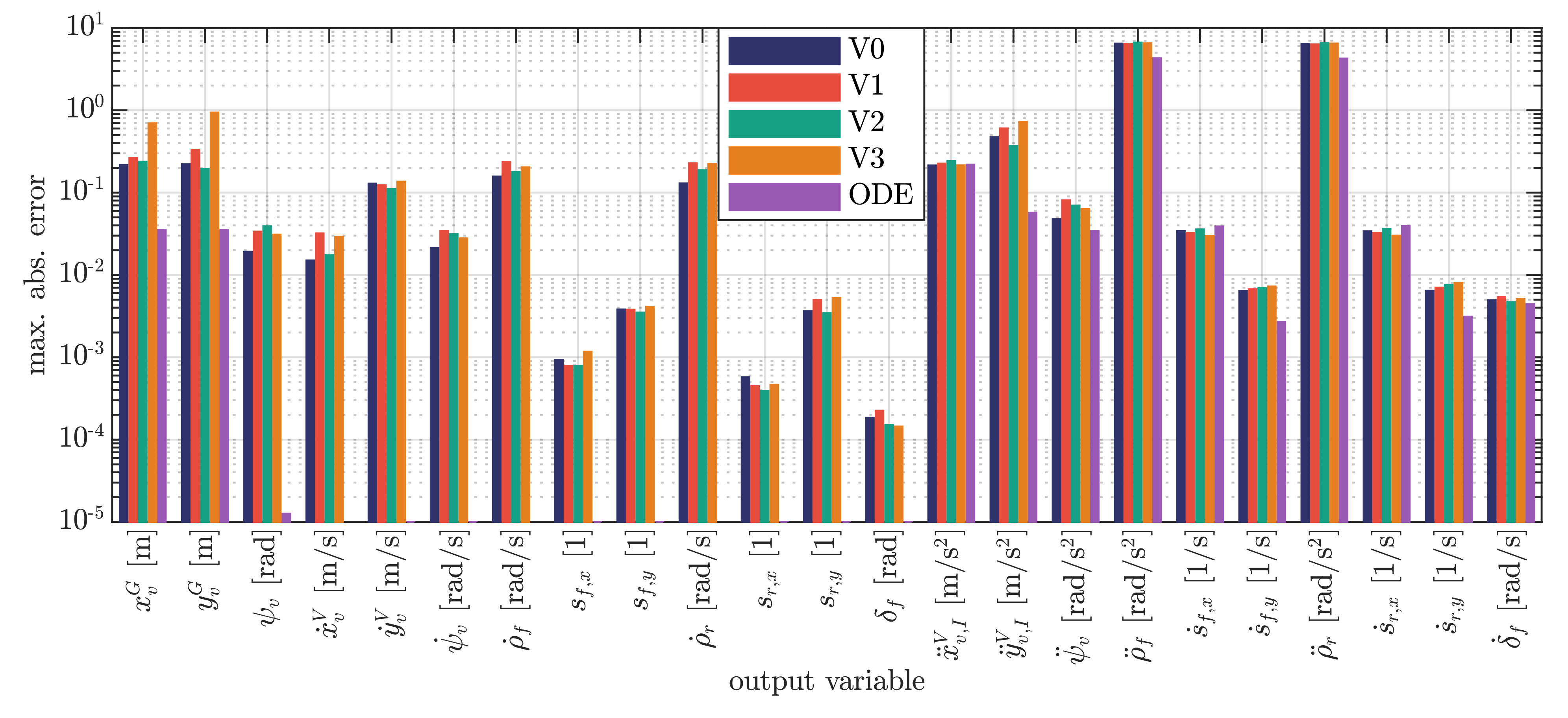
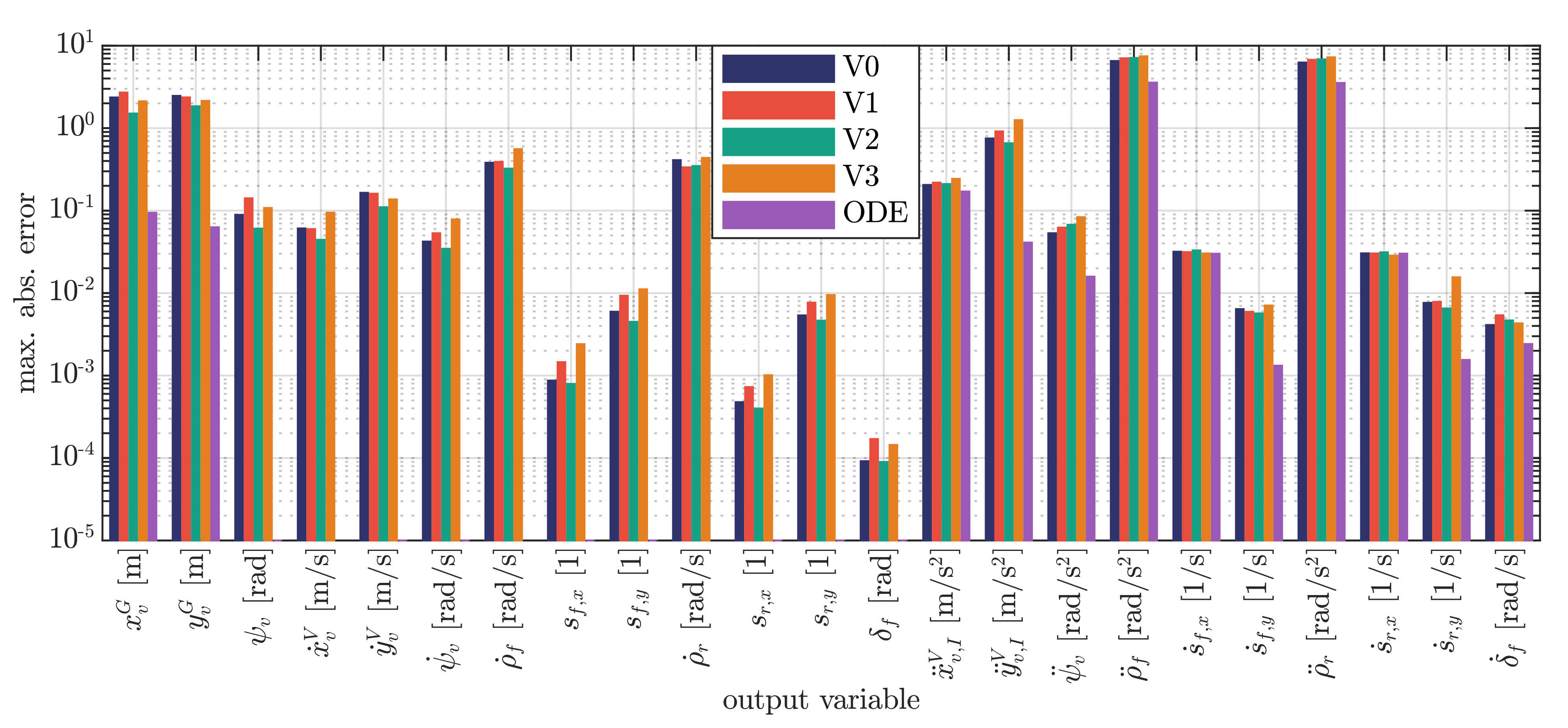
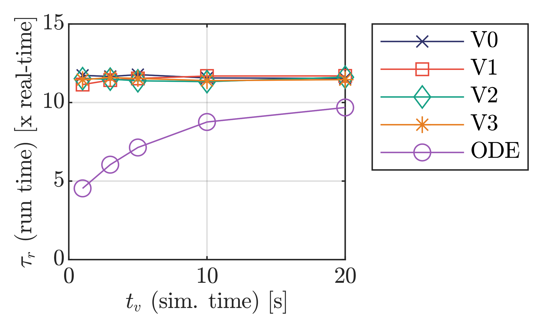
5.3. Evaluation of Input–Output Concept

It is also important to investigate the estimation errors for the whole test dataset to get a complete picture of the proposed method’s performance. To find the best choice of variants V0–3, a comparison of these is also necessary. Figure 8 shows the E_MAX (maximal absolute error) values calculated for the whole test dataset and all vehicle simulation output quantities in case of the different variants V0–3 considering a 3 s long simulation time. Figure 9 shows the same information considering 10 s long simulations. The values labeled with ODE represent the estimation error that is present even if we assume perfect neural network performance. For these data, the worst case, considering the V0 variant with the maximal number of variables obtained by numerical integration, is selected. Please note that a logarithmic scale is used for the axis of error values.

As expected, the magnitude of overall estimation error is growing with the simulation time. On one hand, the value of state variables that are available in the neural network output is calculated by a cumulative sum according to Equation (62). In this way, the estimation error of these values accumulates with the number of steps in the estimation loop. As this cumulative sum of previous network outputs is also used to calculate the input of the network, the error spreads further.

On the other hand, the error of numerical integration for state variables that are not part of the neural network output also increases with the number of integration steps. For the state derivative quantities, the estimation errors’ speed of growth with simulation length is much less, as these are calculated directly from the neural network output.

From comparing the different variants, it is interesting to observe that direct position estimation with the V3 network massively underperforms the other variants with the numerically integrated position in the case of 3 s simulation time. Still, this performance gap disappears in the case of 10 s simulation, as the integration error grows faster. Besides this finding, there is no elementary difference between the performance of different variants. On average, variant V2 performs the best with direct yaw angle estimation and numerical position integration. The maximal position error remains under 1.5 m, and the maximal yaw angle error does not exceed 4${}^{\circ }$ for the complete test dataset. These results are not much worse than the guaranteed performance of fused GNSS (Global Navigation Satellite System), and INS (Inertial Navigation System) localization solutions for global positioning [37]. Naturally, the most significant deviations can be observed in the case of the scenarios that are the most dynamically demanding with the largest longitudinal and lateral accelerations. This meets expectations, since the behavior of the vehicle becomes strongly nonlinear while moving closer to the adhesion limits of the tire–road contact. This nonlinear behavior is then harder to estimate, also because the very high acceleration events are rare compared to the average situations in the simulated realistic driving scenarios. With appropriate safety margins on the position results, the neural-network-based model can be used for simulations of approximately 10 s. For feasibility supervision, the original dynamic model can be used at any time.

Another important aspect of our evaluation is runtime, since the main goal with the presented dynamic-model-based training is to provide faster simulations with the neural-network-based model than with the original one. Figure 10 shows the runtime of the dynamic model and the different neural-network-based variants as to how many times faster they are evaluated than real-time (a ratio of simulated time and runtime). Due to the same total neuron count, almost all variants have the same runtime. Small differences can be observed due to the different number of state variables that have to be calculated by numerical integration. The dynamic model provides better performance with longer simulations because the initialization overhead remains the same in all cases. With short simulation times, the neural network based model is more than two times faster than the original one. Still, the advantage is clearly visible for the total domain of intended usage.

6. Discussion

It is important to discuss the limitations and possible issues of the proposed model. The main use case for the presented method is short-term vehicle motion simulation, particularly for the application in optimization-based motion planning algorithms. Accordingly, the proposed model cannot provide accurate results for simulations longer than approximately 10 s, as the regression error of the neural network is propagated inside the simulation loop.

The learning dataset comes from vehicle dynamics simulations with a planar single track model, which we would like to replace with the neural network based model. This dynamic model provides plausible results in the overwhelming majority of driving scenarios that happen on public roads. However, it also has some important limitations. Vertical dynamic effects such as road unevenness or load transitions due to road slope are not considered. Furthermore, scenarios where the friction conditions are important at all four wheels, such as when the left and right side of the vehicle meets with different road surface, cannot be simulated. The neural-network-based model will accordingly inherit the same limitations.

The driving maneuvers that were used to generate learning data also restrict the capabilities of the trained neural network. Because of this, a great emphasis is put on the definition of realistic random scenarios, which involve calm constant velocity parts and dynamically demanding high acceleration sections as well. However, the training maneuvers do not include parts where the vehicle is sliding or drifting or where the wheels are spinning or locking completely. This means that the neural-network-based model also cannot be expected to provide sufficient precision in such scenarios. The number of learning data is selected in a sense that the length of the resulting training process is feasible for experimenting. To increase the robustness of the proposed model, a final training with even more learning data could be performed as well in the future.

7. Conclusions and Future Work

This paper presents a novel method for short-term (≤10 s) vehicle motion simulation with an artificial neural-network-based approach. Firstly, learning samples are generated based on a classical nonlinear vehicle model for a dynamically diverse set of driving maneuvers. Reference data of these driving maneuvers are created by a numerical motion planning algorithm based on the assignment of piecewise linear travel velocity and curvature profiles similar to public road designs. The input of the trajectory planner is computed randomly to ensure that the resulting motions are realistic and contain demanding high-acceleration cases. Supervised learning techniques are then used to train the fully connected deep neural network to estimate a future state of the vehicle on the basis of its current state and driver inputs. The state variables that are not present in the output of the neural network are subsequently calculated by numerical integration. This algorithm is later used in a feedback loop to simulate the motion of the vehicle over time, where the output of the network is used to calculate its input for the next time step. For short-term simulations, the resulting neural-network based vehicle simulation algorithm is capable of fully replacing the classical dynamic model while being considerably faster. This speed gain can be especially useful in the online optimization loop of dynamically feasible optimal motion planner algorithms, where the required duration of simulations is typically inside the range where the new approach delivers plausible results. In this application, supervision of the neural-network-based results is possible by a one-time execution of the dynamic model.

The proposed algorithms are naturally not perfect. Investigation of the usage of different neural network architectures like cascade neural networks or recurrent neural networks like LSTM (Long Short-Term Memory) to estimate future vehicle state(s) to reach better regression performance would enable longer simulation times; this is a natural extension of the presented work. Another interesting future direction could be the application of transfer learning to adapt the presented model to changing vehicle parameters and friction conditions. As a next step towards a measurement-based training, sensor noises and errors could also be added to the perfect simulation data to examine their effect on the performance of the model. Training the neural networks based on real vehicle measurements afterwards is also an exciting opportunity to provide even more realistic simulations.

References

1. Watzenig, D.; Horn, M. Automated Driving: Safer and More Efficient Future Driving; Springer: Berlin/Heidelberg, Germany, 2016. [Google Scholar]
2. Tettamanti, T.; Varga, I.; Szalay, Z. Impacts of Autonomous Cars from a Traffic Engineering Perspective. Period. Polytech. Transp. Eng. 2016, 44, 244–250. [Google Scholar] [CrossRef] [Green Version]
3. Barsi, Á.; Csepinszky, A.; Lógó, J.; Krausz, N.; Potó, V. The Role of Maps in Autonomous Driving Simulations. Period. Polytech. Transp. Eng. 2020, 48, 363–368. [Google Scholar] [CrossRef]
4. Colan, J.; Nakanishi, J.; Aoyama, T.; Hasegawa, Y. Optimization-Based Constrained Trajectory Generation for Robot-Assisted Stitching in Endonasal Surgery. Robotics 2021, 10, 27. [Google Scholar] [CrossRef]
5. Beschi, M.; Mutti, S.; Nicola, G.; Faroni, M.; Magnoni, P.; Villagrossi, E.; Pedrocchi, N. Optimal Robot Motion Planning of Redundant Robots in Machining and Additive Manufacturing Applications. Electronics 2019, 8, 1437. [Google Scholar] [CrossRef] [Green Version]
6. Zhang, X.; Ming, Z. Trajectory Planning and Optimization for a Par4 Parallel Robot Based on Energy Consumption. Appl. Sci. 2019, 9, 2770. [Google Scholar] [CrossRef] [Green Version]
7. Howard, T.M.; Kelly, A. Optimal rough terrain trajectory generation for wheeled mobile robots. Int. J. Robot. Res. 2007, 26, 141–166. [Google Scholar] [CrossRef]
8. Urmson, C.; Anhalt, J.; Bagnell, D.; Baker, C.; Bittner, R.; Clark, M.N.; Dolan, J.; Duggins, D.; Galatali, T.; Ferguson, D.; et al. Autonomous driving in urban environments: Boss and the urban challenge. J. Field Robot. 2008, 25, 425–466. [Google Scholar] [CrossRef] [Green Version]
9. Ajanovic, Z.; Lacevic, B.; Shyrokau, B.; Stolz, M.; Horn, M. Search-Based Optimal Motion Planning for Automated Driving. In Proceedings of the 2018 IEEE/RSJ International Conference on Intelligent Robots and Systems (IROS), Madrid, Spain, 1–5 October 2018; pp. 4523–4530. [Google Scholar] [CrossRef] [Green Version]
10. Diachuk, M.; Easa, S.M.; Bannis, J. Path and Control Planning for Autonomous Vehicles in Restricted Space and Low Speed. Infrastructures 2020, 5, 42. [Google Scholar] [CrossRef]
11. Hegedus, F.; Bécsi, T.; Aradi, S.; Szalay, Z.; Gáspár, P. Real-time optimal motion planning for automated road vehicles. In Proceedings of the 21th IFAC World Congress, Berlin, Germany, 12–17 July 2020; pp. 15856–15861. [Google Scholar]
12. Bender, J.; Müller, M.; Macklin, M. Position-Based Simulation Methods in Computer Graphics. Eurographics 2015. [Google Scholar] [CrossRef]
13. Müller, M.; Heidelberger, B.; Hennix, M.; Ratcliff, J. Position based dynamics. J. Vis. Commun. Image Represent. 2007, 18, 109–118. [Google Scholar] [CrossRef] [Green Version]
14. Harmon, D.; Zorin, D. Subspace integration with local deformations. ACM Trans. Graph. (TOG) 2013, 32, 1–10. [Google Scholar] [CrossRef]
15. von Radziewsky, P.; Eisemann, E.; Seidel, H.P.; Hildebrandt, K. Optimized subspaces for deformation-based modeling and shape interpolation. Comput. Graph. 2016, 58, 128–138. [Google Scholar] [CrossRef]
16. Xu, W.; Umetani, N.; Chao, Q.; Mao, J.; Jin, X.; Tong, X. Sensitivity-optimized rigging for example-based real-time clothing synthesis. ACM Trans. Graph. 2014, 33, 107:1–107:11. [Google Scholar] [CrossRef]
17. Luo, R.; Shao, T.; Wang, H.; Xu, W.; Chen, X.; Zhou, K.; Yang, Y. NNWarp: Neural network-based nonlinear deformation. IEEE Trans. Vis. Comput. Graph. 2018, 26, 1745–1759. [Google Scholar] [CrossRef] [Green Version]
18. Holden, D.; Duong, B.C.; Datta, S.; Nowrouzezahrai, D. Subspace neural physics: Fast data-driven interactive simulation. In Proceedings of the 18th annual ACM SIGGRAPH/Eurographics Symposium on Computer Animation, Los Angeles, CA, USA, 26–28 July 2019; pp. 1–12. [Google Scholar]
19. Hu, S.; d’Ambrosio, S.; Finesso, R.; Manelli, A.; Marzano, M.R.; Mittica, A.; Ventura, L.; Wang, H.; Wang, Y. Comparison of Physics-Based, Semi-Empirical and Neural Network-Based Models for Model-Based Combustion Control in a 3.0 L Diesel Engine. Energies 2019, 12, 3423. [Google Scholar] [CrossRef] [Green Version]
20. Guarneri, P.; Rocca, G.; Gobbi, M. A Neural-Network-Based Model for the Dynamic Simulation of the Tire/Suspension System While Traversing Road Irregularities. IEEE Trans. Neural Netw. 2008, 19, 1549–1563. [Google Scholar] [CrossRef]
21. Liu, X.; Hu, D.; Xiao, J.; Hu, J. Modeling and simulation on movement of air cushion vehicle based on neural network. In Proceedings of the 2017 2nd International Conference on Robotics and Automation Engineering (ICRAE), Shanghai, China, 29–31 December 2017; pp. 513–516. [Google Scholar]
22. Swain, S.K.; Rath, J.J.; Veluvolu, K.C. Neural Network Based Robust Lateral Control for an Autonomous Vehicle. Electronics 2021, 10, 510. [Google Scholar] [CrossRef]
23. He, Z.; Nie, L.; Yin, Z.; Huang, S. A two-layer controller for lateral path tracking control of autonomous vehicles. Sensors 2020, 20, 3689. [Google Scholar] [CrossRef]
24. Song, S.; Chen, H.; Sun, H.; Liu, M. Data Efficient Reinforcement Learning for Integrated Lateral Planning and Control in Automated Parking System. Sensors 2020, 20, 7297. [Google Scholar] [CrossRef]
25. Hu, H.; Lu, Z.; Wang, Q.; Zheng, C. End-to-End Automated Lane-Change Maneuvering Considering Driving Style Using a Deep Deterministic Policy Gradient Algorithm. Sensors 2020, 20, 5443. [Google Scholar] [CrossRef]
26. Hegedüs, F.; Bécsi, T.; Aradi, S.; Gáspár, P. Motion Planning for Highly Automated Road Vehicles with a Hybrid Approach Using Nonlinear Optimization and Artificial Neural Networks. Stroj. Vestn. J. Mech. Eng. 2019, 65, 148–160. [Google Scholar] [CrossRef]
27. Kovári, B.; Hegedüs, F.; Bécsi, T. Design of a Reinforcement Learning-Based Lane Keeping Planning Agent for Automated Vehicles. Appl. Sci. 2020, 10, 7171. [Google Scholar] [CrossRef]
28. Hegedüs, F.; Bécsi, T.; Aradi, S.; Gáspár, P. Model based trajectory planning for highly automated road vehicles. IFAC-PapersOnLine 2017, 50, 6958–6964. [Google Scholar] [CrossRef]
29. Schramm, D.; Hiller, M.; Bardini, R. Vehicle Dynamics; Springer: Berlin/Heidelberg, Germany, 2014. [Google Scholar]
30. Luhua, Z.; Qinggui, C.; Yushan, L.; Naixiu, G. An optimization technique of braking force distribution coefficient for truck. In Proceedings of the 2011 International Conference on Transportation, Mechanical, and Electrical Engineering (TMEE), Changchun, China, 16–18 December 2011; pp. 1784–1787. [Google Scholar]
31. Hall, D.E.; Moreland, J.C. Fundamentals of rolling resistance. Rubber Chem. Technol. 2001, 74, 525–539. [Google Scholar] [CrossRef]
32. Pacejka, H.B. Tire and Vehicle Dynamics, 3rd ed.; Butterworth-Heinemann: Oxford, UK, 2012; pp. 355–401. [Google Scholar] [CrossRef]
33. Snider, J.M. Automatic Steering Methods for Autonomous Automobile Path Tracking; CMU-RITR; Robotics Institute: Pittsburgh, PA, USA, 2009. [Google Scholar]
34. Cantisani, G.; Del Serrone, G. Procedure for the Identification of Existing Roads Alignment from Georeferenced Points Database. Infrastructures 2021, 6, 2. [Google Scholar] [CrossRef]
35. Parlangeli, G.; Ostuni, L.; Mancarella, L.; Indiveri, G. A motion planning algorithm for smooth paths of bounded curvature and curvature derivative. In Proceedings of the 2009 17th Mediterranean Conference on Control and Automation, Thessaloniki, Greece, 24–26 June 2009; pp. 73–78. [Google Scholar]
36. Kingma, D.P.; Ba, J. Adam: A method for stochastic optimization. arXiv 2014, arXiv:1412.6980. [Google Scholar]
37. Dong, Y.; Wang, D.; Zhang, L.; Li, Q.; Wu, J. Tightly Coupled GNSS/INS Integration with Robust Sequential Kalman Filter for Accurate Vehicular Navigation. Sensors 2020, 20, 561. [Google Scholar] [CrossRef] [Green Version]
Figure 1. Progress of presented research.
Electronics 10 00928 g001
Figure 2. Nonlinear single track vehicle model.
Electronics 10 00928 g002
Figure 3. Motion planning input and output.
Electronics 10 00928 g003
Figure 4. Random trajectories.
Electronics 10 00928 g004
Figure 5. Learning progress of neural network.
Electronics 10 00928 g005
Figure 6. Regression fit of the trained neural network.
Electronics 10 00928 g006
Figure 7. Motion prediction with trained neural network.
Electronics 10 00928 g007
Figure 8. Maximum estimation error of neural network based models for 3 s simulation.
Electronics 10 00928 g008
Figure 9. Maximum estimation error of neural network based models for 10 s simulation.
Electronics 10 00928 g009
Figure 10. Runtime of neural-network-based models.
Electronics 10 00928 g010