Abstract
The paper presents considerations concerning the transfer of random errors from the input to the output of the Discrete Wavelet Transform (DWT) algorithm. The concept of determining an uncertainty of its output data based on the probabilistic error description has been presented. The DWT is discussed as the product of the vector of input quantities and the matrix of algorithm coefficients. Calculations of the uncertainty of a single output result of the algorithm are described with assumption that the input quantities are burdened by random errors of known distributions. Theoretical considerations have been verified by simulation experiments using the Monte Carlo method. Determining the uncertainty at the DWT output is possible due to the specific properties of transferring random errors by linear and additive algorithms.
1. Introduction
Currently, digital data processing algorithms are an indispensable part of most measurement systems [1]. In order to determine whether a measuring chain fulfills its task correctly, it is necessary to know the metrological properties of every hardware/software component. Due to the large complexity, the analysis of properties of measuring chains containing elements of digital data processing is often omitted in many systems focused on wavelet transform applications [2,3]. Analytic uncertainty analysis methods such as these described in [4,5] are too complex and time-consuming to be used universally in common measuring chain applications. However, the method described in the paper can be used in most cases in which the functioning of the algorithm is not fully known and the algorithm itself becomes a kind of “black box” [6].
This article will describe the general signal processing structure, bases of wavelet transform algorithm and its matrix. After introducing this elements-uncertainty calculation method will be described. To prove the validity of described method Monte Carlo simulations will be presented. Finally, the presented method will be compared with other methods to demonstrate its advantages, and some examples of its applications will also be presented.
To consider the error propagation, the general structure of a measuring chain shown in Figure 1 is taken into account.
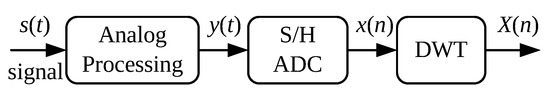
Figure 1.
The general structure of the analyzed signal processing chain.
In a general case, the numerical operation performed by a data processing algorithm can be presented in the matrix form [7]. For this purpose, it is necessary to identify the algorithm coefficients. This procedure allows us to analyze the properties of the algorithm without knowing its exact structure. The specificity of the Discrete Wavelet Transform (DWT) algorithm is that its operation depends on the choice of the parameter of the filter bank [8,9]; therefore, the analytical approach to the problem under consideration becomes extremely difficult [10]. In the case of an analytical approach, any modification of algorithm parameters such as mother wavelet, decomposition level, number of input samples, requires problem re-analysis. This situation is problematic in a measuring chain design because these parameters are changed in the design process and the uncertainty analysis must be repeated. The method described in this paper enables the analysis of any combination of the filter bank and requires only identification of the algorithm coefficients matrix.
2. Wavelet Transform Algorithm
The wavelet transform (WT) algorithm is a tool enabling the analysis of signals by presenting them using a scaled and time-shifted function called a “mother wavelet” [11]. This technique provides the possibility to analyze the signal simultaneously in the time and frequency domain, similar to the “Short-time Fourier Transform”. Generally, the WT can be expressed by the following equation:
in which c is a WT coefficient, a is the scale parameter, b is the shift (position) parameter and –mother wavelet.
Equation (1) describes a filter whose parameters and input window depend on the scale parameter a and the time shift parameter b. The scale parameter a is related to the frequency. The higher the value of the parameter , the more “extended” the wavelet becomes, which corresponds to the lower frequency values. In the case of smaller values of the coefficient , the wavelet is “compressed”, which corresponds to the higher frequency of harmonics. The time shift parameter b sets the time window for the analyzed input signal.
In the case of continuous wavelet transform (CWT), the scale and shift parameters can assume any value, which makes it possible to determine an infinite number of transformation coefficients. By entering the limitation, where , and , the equation describing the DWT is obtained. This is necessary to limit the number of transform coefficients to a value sufficient to correctly reconstruct the processed signal.
The selection of the mother wavelet is a key issue when using the WT algorithm. Many different kinds of wavelets are described in publications, depending on their specificity and properties, they are used to analyze and process measuring signals. The paper presents the wavelets of the “Daubechies” family (“db”) [12] and their derivatives “Symlet” (“sym”) (used, among others, for image and sound analysis [13]) as well as wavelets of the “Spline” family [14] (used, among others, for the analysis of the condition of machine mechanical elements [15]). In addition, a concept using double-density decomposition (“dden”) [16] will be analyzed. This concept is often used to remove noise from the measured signal [17]. The selection of wavelets aims to show the universality of the method presented in this paper.
3. Matrix Form of the DWT Algorithm
The general purpose of the algorithm under consideration is to convert the input quantity given as series of samples , where n is an input sample number, into series of samples of the output quantity denoted as , where m is an output sample number. The discussed algorithm operates on a sequence of N samples of the input quantity and returns the sequence of M values of the output quantity. Therefore, the algorithm can be described by the general matrix equation [6,7]:
By introducing designations, where is a vector of output quantities, is a vector of input quantities and is a matrix of algorithm coefficients, Equation (2) can be presented in the form:
By substituting vector x into the input of the algorithm and values of subsequent elements of this vector are determined in accordance with the equation:
the coefficients of the i-th column of matrix can be identified. By executing N iterations (for ), the values of all elements of matrix are obtained [18].
This method eliminates the need to know the exact structure of the DWT algorithm and enables uniform analysis for any set of filter banks.
4. Relationship between Data Uncertainty at the Input and Output of the Algorithm
According to the considerations presented in [19], it is possible to determine the relationship between error variances at the output and at the input of the algorithm presented in the matrix form. A single output result of the algorithm for the i-th row of the matrix of coefficients is described by the equation:
Random error appearing at the output of the algorithm in the i-th step of its implementation can be presented as a linear combination of the input random error and algorithm coefficients:
By executing the algorithm repeatedly, a set of output errors with variance is obtained. This is related to the variance of the set of input errors by the relationship:
which is obtained assuming that the values of the input error are not correlated with each other. Denoting the sum of the squares of the i-th row of matrix as:
the relationship between the variance of random error at the output and at the input of the algorithm takes the form:
Assuming that each subsequent value of the algorithm output quantity can be considered as a result of the single-point algorithm (5) [7,18,19], the shown relationship is determined separately for each result of the vector, taking into account the corresponding row of the matrix.
According to the central limit theorem, regardless of the distribution of input errors, it can be assumed that the error distribution at the output of the algorithm will have (with an acceptable approximation) the shape of the normal distribution [20]. Assuming the uncertainty at a 95% confidence level, a standard deviation can be used to determine it [7,19,20]:
where is a coverage factor.
Thus, it is possible to define the uncertainty transfer coefficient for various types of random errors as:
For example, for input random errors with uniform distribution (coverage factor at 95% confidence level), the uncertainty transfer coefficient will be:
while for input errors described by a normal distribution it is:
On the basis of the presented information, it can be observed that knowledge of the matrix coefficients and the parameters of input uncertainty sources allows us to determine the uncertainty of the output quantities of the algorithm and as a result, the uncertainty of the output quantities of the whole measuring chain.
In the case of wavelets from the “db” and “sym” family, regardless of the other parameters of the decomposition process, the value of the coefficient for each row of matrix is equal to 1 [12]. This means that the algorithm transfers random errors which have a normal distribution with the coefficient . For the other considered wavelets, the value of the coefficient depends on the number of iterations of the decomposition process, the length of the input vector and on the index of the output value of the algorithm.
5. Propagation of Normal Distribution Error
White noise is an example of an error source with a normal distribution. Knowing the noise parameters and assuming that it is the dominant source of error, it is possible to determine the uncertainty of a sample of the algorithm output quantity on the basis of Equation (13).
In order to perform the appropriate calculations, it was assumed that at the input of the DWT algorithm is given a vector consisting of samples of the input quantity. Table 1 presents the values of the uncertainty transfer coefficient for the 50th element of the DWT algorithm output vector, depending on the mother wavelet and the number of decomposition levels.

Table 1.
Values of the uncertainty transfer coefficient of the Discrete Wavelet Transform (DTW) algorithm depending on the type of wavelet and the number of decomposition levels for errors which have normal distribution.
Table 2 shows the uncertainty values calculated and obtained by Monte Carlo method for the 50th element of the DWT output vector in the case of input data with added white noise with variance for exemplary mother wavelets and decomposition levels. In order to verify the correctness of the calculated uncertainty values, the Monte Carlo method was used and 1,000,000 iterations of calculating the value of the output quantity were made, then the uncertainty was determined based on the histogram of the error. Figure 2 shows an example of the input and output quantity errors histograms for “spline4:4” wavelet and four levels of decomposition.
Table 2.
Examples of the output uncertainty values (—calculated; —simulated) in the case of added white noise with variance ).
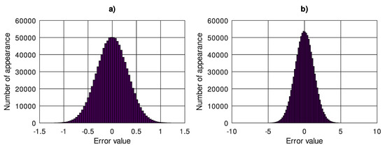
Figure 2.
Histogram of the (a) input quantity error, (b) output quantity error, wavelet “spline4:4”, four levels of decomposition.
6. Propagation of Uniform Distribution Error
An example of an error with a uniform distribution is the quantization error of the ADC. Assuming that a 10-bit converter () with the processing range V and V has been used, the quantum value can be calculated as V. In this case, the uncertainty of the algorithm input data is V and the standard deviation: V. Assuming that the quantization error of the ADC is dominant in the situation under consideration, it is possible to determine the uncertainty of subsequent elements of the vector of the algorithm output quantity on the basis of Equation (12). Table 3 presents the values of the uncertainty transfer coefficient for the 50th element of the DWT algorithm output vector, depending on the mother wavelet and the number of decomposition levels.
Table 3.
Values of the uncertainty transfer coefficient of the DTW algorithm depending on the type of wavelet and the number of decomposition levels for errors with uniform distribution.
Table 4 shows the uncertainty values calculated and obtained by Monte Carlo method for the 50th element of the DWT output vector in the case of input data with added quantization noise with variance for exemplary mother wavelets and decomposition levels. In order to verify the correctness of the calculated uncertainty values, the Monte Carlo method was used and 1,000,000 iterations of calculating the value of the output quantity were made, then the uncertainty was determined based on the histogram of the error. Figure 3 shows an example of the input and output quantity errors histograms for “spline4:4” wavelet and four levels of decomposition.
Table 4.
Examples of the output uncertainty values (—calculated; —simulated) in the case of added errors with uniform distribution and variance .
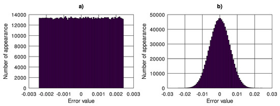
Figure 3.
Histogram of the (a) input quantity error, (b) output quantity error, wavelet “spline4:4”, four levels of decomposition.
7. Multiple Error Sources
In the case of multiple error sources, the presented method also can be applied. In the first step, there is a need to calculate the input quantity error distribution parameters: variance and coverage factor. These parameters can be calculated analytically [19] or found using the Monte Carlo method [21]. The analytic method can be easily applied in the case of standard error distributions while the Monte Carlo method is more universal, but requires time to compute.
Assuming a measurement chain containing the AD converter described in the previous chapter and an analog part where the white noise is present, the Monte Carlo method can be applied to find the parameters of input values error distribution. In this case, the sources of errors have uniform distribution with coverage factor , variance and normal distribution with coverage factor , variance . Because the considered error distributions are standard, the analytic method described in [19] can also be easily applied, but in order to emphasize the universality of the presented method, the Monte Carlo method is taken under consideration. In the case of more than two error sources, the analytic method might be not applicable.
Figure 4a presents a histogram of the input quantity error in the described case. Assuming the uncertainty at 95% confidence level according to the data presented in Figure 4a, the variance of input quantity error , coverage factor and uncertainty . According to Equations (10) and (11) and the calculated input error distribution parameters, the uncertainty transfer coefficient for i-th output quantity can be defined as:
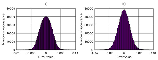
Figure 4.
Histogram of the (a) input quantity error, (b) output quantity error, wavelet “spline4:4”, four levels of decomposition.
Table 5 presents the values of the uncertainty transfer coefficient for the 50th element of the DWT algorithm output vector, depending on the mother wavelet and the number of decomposition levels. Table 6 shows the uncertainty values calculated according to Equation (10) and obtained by the Monte Carlo method for the 50th element of the DWT output vector in the described case. Figure 4b shows an example of the output quantity error histogram for “spline4:4” wavelet and four levels of decomposition.
Table 5.
Values of the uncertainty transfer coefficient of the DTW algorithm depending on the type of wavelet and the number of decomposition levels for two error sources.
Table 6.
Examples of the output uncertainty values in the case of two error sources.
8. Results Interpretation
In the case of “db” and “sym” wavelet family, propagation of the random errors is always the same regardless of any other algorithm parameters. For the “dden” wavelet family, the uncertainty transfer coefficient depends on the decomposition level. For decomposition levels 2 and 4 it is about 1 (1.027, 1.026), for higher levels, 6 and 8, it is less than 1. This means that for this family of wavelets, random errors are not amplified from input to output of the DWT algorithm, and for higher levels of decomposition, these errors are suppressed. In case of “spline” wavelet families uncertainty transfer coefficient is always more than 1, and is strongly related to the number of decomposition iterations and the wavelet form. It should be mentioned that the uncertainty transfer coefficient in most cases changes for different elements of the output vector, because the coefficient A depends on a single row of the matrix.
It is very important to remember that values presented in this article are results for a single output quantity. To consider other outputs quantities uncertainty, coefficients for all other i values must be calculated in the described way.
9. Comparison with Other Methods
Currently, the two most common methods used to determine the uncertainty of the output quantities in the case of measurement chains containing the DWT algorithm can be mentioned in the literature. These include the analytical methods described, e.g., in [4,5,22] and the Monte Carlo method, which is one of the most universal methods of uncertainty determination [21].
Analytical methods require precise knowledge of the applied mother’s wavelet, therefore any change of this parameter is connected with the necessity to perform a repeated analysis. Moreover, these methods are complex and time-consuming. Usually, the user will use ready-made tools implementing the DWT algorithm, such as Matlab or GNU/Octave, so the exact form of the algorithm may not be fully known. Hence, in practice, analytical methods are relatively rarely used.
The Monte Carlo method turns out to be more universal and easier to apply. For this method, it is not necessary to know the structure of the algorithm or the form of the used mother’s wavelet. However, it requires a lot of computational expenditure and the preparation of an appropriate simulation, which assumes the presence of all considered error sources. Two measuring chains should then be designed, the first one-ideal (without errors) and the second one, in which these errors occur. After the simulation, the algorithm’s output uncertainty can be estimated based on the histogram of errors.
It should be noted that in the case of both discussed methods, the analysis will concern a single output quantity of the measurement chain. In real measurement chains, the control decision is made on the basis of several quantities, therefore an uncertainty analysis should be performed for each of them. In the case of the author’s method presented in this paper, these inconveniences do not occur. In order to determine the uncertainty of any output quantity, it is only necessary to calculate the appropriate coefficient for that quantity and apply Equation (11). Possible changes of the DWT algorithm parameters require only determine the new values of the matrix , as shown earlier dependencies. Compared to the analytical method, the approach presented by the authors does not require a complicated analysis of the selected mother’s wavelet, knowledge of the form of the algorithm, or its numerical structure. Moreover, its use is not time-consuming. On the other hand, unlike the Monte Carlo method, a possible change of the algorithm parameters does not require repeating time-consuming simulations.
However, the presented method has a few limitations. In order to use it, it is necessary to know the parameters of the error distribution at the algorithm input. In the case of many sources of error, these parameters can be determined by the analytical method [19] or by simulation, as shown in this paper. Moreover, the error values of all input quantities cannot be correlated with each other [7].
10. Examples of Applications
As the wavelet transform is applied to signal processing and analysis in many areas, the presented method can find a variety of applications. The literature describes many applications containing the DWT algorithms [2,3,13,15], however, they do not include the metrological analysis necessary to determine the properties of the measurement chain. This may be due to the drawbacks of the previously discussed methods of uncertainty analysis of the DWT algorithms.
In the case described in [15], the uncertainty of the analog part of the measurement chain should be determined and then the uncertainty of the input quantities of the wavelet transformation algorithm should be determined taking into account the digital part of the measurement chain. This example shows the applicability and advantages of the developed method. It should be emphasized that the mentioned application contains solutions for several combinations of parameters of the DWT algorithm in order to determine which set of parameters is the most appropriate. In this case, the universality and speed of implementation of the developed method become very valuable advantages.
Another example of the application of the described method may be sound processing measurement chains, such as speech recognition algorithms or other applications described, among others, in [2]. In this case, the metrological analysis must take into account the parameters of the analog part of the measurement chain: the converter (microphone), cabling, possible filters and the digital part: the A/D converter, additional filtering algorithms or initial signal processing. The determined parameters of the discrete transformation algorithm input quantities errors can be used to determine the uncertainty of the output quantities of the analyzed measurement chain. A similar situation occurs in the case of image analysis algorithms [9,11].
11. Conclusions
The presented method of calculating the uncertainty of the DWT algorithm output quantities, described for the universal case in [6,7,18], gives results similar to those obtained in the simulation. It allows us to determine the metrological properties of DWT algorithms for any filter bank set and any number of decomposition levels.
The described method allows us to determine the uncertainty of the output quantity of the DWT algorithm related to the corresponding frequency range and time interval. This method assumes that the parameters related to the sample are ideal and any processed errors are reflected in the sample values. The uncertainty in determining the frequency range or the time interval is therefore included in the uncertainty of the value of the output quantity [6,7,18]. It unifies the process of determining the uncertainty of the input quantity in the case of various sources of errors and the analysis of their impact on the uncertainty of the output quantity.
In order to determine the uncertainty in case of several types of errors, the analysis should be extended by determining the convolution of the probability density functions or application of a reductive interval arithmetic [19,23]. For errors with a non-standard probability distribution, the presented method is not directly applicable. In this case, the Monte Carlo method can be used [21,24] to determinate input error distribution parameters in order to apply the presented method.
Author Contributions
Data curation, Ł.D.; formal analysis, J.R.; funding acquisition, Ł.D.; investigation, Ł.D.; methodology, J.R.; project administration, J.R.; software, Ł.D.; supervision, J.R.; writing—original draft preparation, Ł.D. and J.R; writing—review and editing, Ł.D. and J.R. Both authors have read and agreed to the published version of the manuscript.
Funding
This research received no external funding.
Data Availability Statement
Data available on request.
Conflicts of Interest
The authors declare no conflict of interest.
Abbreviations
The following abbreviations are used in this manuscript:
| WT | Wavelet transform |
| CWT | Continuous wavelet transform |
| DWT | Discrete wavelet transform |
References
- Axelsson, E.; Claessen, K.F. A domain specific language for digital signal processing algorithms. In Proceedings of the Eighth ACM/IEEE International Conference on Formal Methods and Models for Codesign, Grenoble, France, 26–28 July 2010. [Google Scholar] [CrossRef]
- Wang, Y.S. Sound quality estimation for nonstationary vehicle noises based on discrete wavelet transform. J. Sound Vib. 2009, 324, 1124–1140. [Google Scholar] [CrossRef]
- Ocak, H. Automatic detection of epileptic seizures in EEG using discrete wavelet transform and approximate entropy. Expert Syst. Appl. 2009, 36, 2027–2036. [Google Scholar] [CrossRef]
- Yan, B.F.; Miyamoto, A.; Brühwilerb, E. Wavelet transform-based modal parameter identification considering uncertainty. J. Sound Vib. 2006, 291, 285–301. [Google Scholar] [CrossRef]
- Wilczok, E. New Uncertainty Principles for the Continuous Gabor Transform and the Continuous Wavelet Transform. Doc. Math. 2000, 5, 201–226. [Google Scholar]
- Konopka, K.; Topór-Kamiński, T. Uncertainty evaluation of measurement data processing algorithm based on its matrix form. Actaphysicapolonica A 2011, 120, 666–670. [Google Scholar] [CrossRef]
- Jakubiec, J. The error based model of a single measurement result in uncertainty calculation of the mean value of series. Probl. Prog. Metrol. 2015, 20, 75–78. [Google Scholar]
- Narang, S.K.; Ortega, A. Perfect reconstruction two-channel wavelet filter banks for graph structured data. IEEE Trans. Signal Process. 2012, 60, 2786–2799. [Google Scholar] [CrossRef]
- Kotteri, K.A.; Bell, A.E.; Carletta, J.E. Design of multiplierless, high-performance, wavelet filter banks with image compression applications. IEEE Trans. Circuits Syst. Regul. Pap. 2004, 51, 483–494. [Google Scholar] [CrossRef]
- Peretto, L.; Sasdelli, R.; Tinarelli, R. On Uncertainty in Wavelet-Based Signal Analysis. Instrum. Meas. IEEE Trans. 2005, 54, 1593–1599. [Google Scholar] [CrossRef]
- Addison, P.S. The Illustrated Wavelet Transform Handbook: Introductory Theory and Applications in Science, Engineering, Medicine and Finance; CRC Press: Boca Raton, FL, USA, 2017. [Google Scholar] [CrossRef]
- Vonesch, C.; Blu, T.; Unser, M. Generalized Daubechies wavelet families. IEEE Trans. Signal Process. 2007, 55, 4415–4429. [Google Scholar] [CrossRef]
- Reddy, B.E.; Narayana, K.V. A lossless image compression using traditional and lifting based wavelets. Signal Image Process. 2012, 3, 213. [Google Scholar] [CrossRef]
- Wang, J. On Spline Wavelets; Sam Houston State University: Huntsville, TX, USA, 2006. [Google Scholar]
- Katunin, A.; Korczak, A. The possibility of application of B-spline family wavelets in diagnostic signal processing. Acta Mech. Autom. 2009, 3, 43–48. [Google Scholar]
- Selesnick, I.W. The double-density dual-tree DWT. IEEE Trans. Signal Process. 2004, 52, 1304–1314. [Google Scholar] [CrossRef]
- Vimala, C.; Priya, P.A. Noise reduction based on Double Density Discrete Wavelet Transform. In Proceedings of the International Conference on Smart Structures and Systems, Chennai, India, 9 October 2014; pp. 15–18. [Google Scholar] [CrossRef]
- Jakubiec, J.; Topór-Kaminski, T. Uncertainty modeling method of data series processing algorithms. In Proceedings of the IMEKO TC-4 Symposium on Development in Digital Measuring Instrumentation and 3rd Workshop on ADC Modelling and Testing, Lisabona, Portugal, 17–18 September 1998. [Google Scholar]
- Jakubiec, J. Reductive interval arithmetic application to uncertainty calculation of measurement result burdened correlated errors. Metrol. Meas. Syst. 2003, 20, 137–156. [Google Scholar]
- Evaluation of Measurement Data—Guide to the Expression of Uncertainty in Measurement; JCGM: Paris, France, 2008.
- Roj, J. Estimation of the artificial neural network uncertainty used for measurand reconstruction in a sampling transducer. IET Sci. Meas. Technol. 2013, 8, 1–7. [Google Scholar] [CrossRef]
- Sarrafi, A.; Mao, Z.; Shiao, M. Uncertainty quantification framework for wavelet transformation of noise-contaminated signals. Measurement 2017, 137, 102–115. [Google Scholar] [CrossRef]
- Batko, W.; Pawlik, P. Uncertainty evaluation in modelling of acoustic phenomena with uncertain parameters using interval arithmetic. Actaphys.-Ser. A Gen. Phys. 2012, 121, A152. [Google Scholar] [CrossRef]
- Janssen, H. Monte-Carlo based uncertainty analysis: Sampling efficiency and sampling convergence. Reliab. Eng. Syst. Saf. 2013, 109, 123–132. [Google Scholar] [CrossRef]
Publisher’s Note: MDPI stays neutral with regard to jurisdictional claims in published maps and institutional affiliations. |
© 2021 by the authors. Licensee MDPI, Basel, Switzerland. This article is an open access article distributed under the terms and conditions of the Creative Commons Attribution (CC BY) license (http://creativecommons.org/licenses/by/4.0/).