
Identification of Degrading Effects in the Operation of Neighboring Photovoltaic Systems in Urban Environments


Abstract
1. Introduction
- Methods for PV system performance assessment based on the temporal analysis of PV system performance metric parameters enable automated detection and identification of different degrading effects causing system faults and underperformance;
- Despite the heterogeneity of PV systems and their properties, the presented methodology uniformly integrates and utilizes underlying methods used for solar irradiance measurement or assessment;
- The proposed performance assessment methodology is seen as a part of automated monitoring and maintenance services and supplementary to periodic on-site inspections;
- The adopted tiered architectural style and fog computing approach enable a scalable solution for the seamless integration of large numbers of distributed PV systems in urban environments, which is in line with the requirements of smart city concepts;
- Cross-correlation-based services and corresponding system-level parameters enable the discovery of erroneous measurements and sensor and operational faults, improving the reliability of information and the accuracy of performance assessment.
2. Related Work
3. Methodology and System Overview
3.1. Methodology Background
3.2. Identification Methods
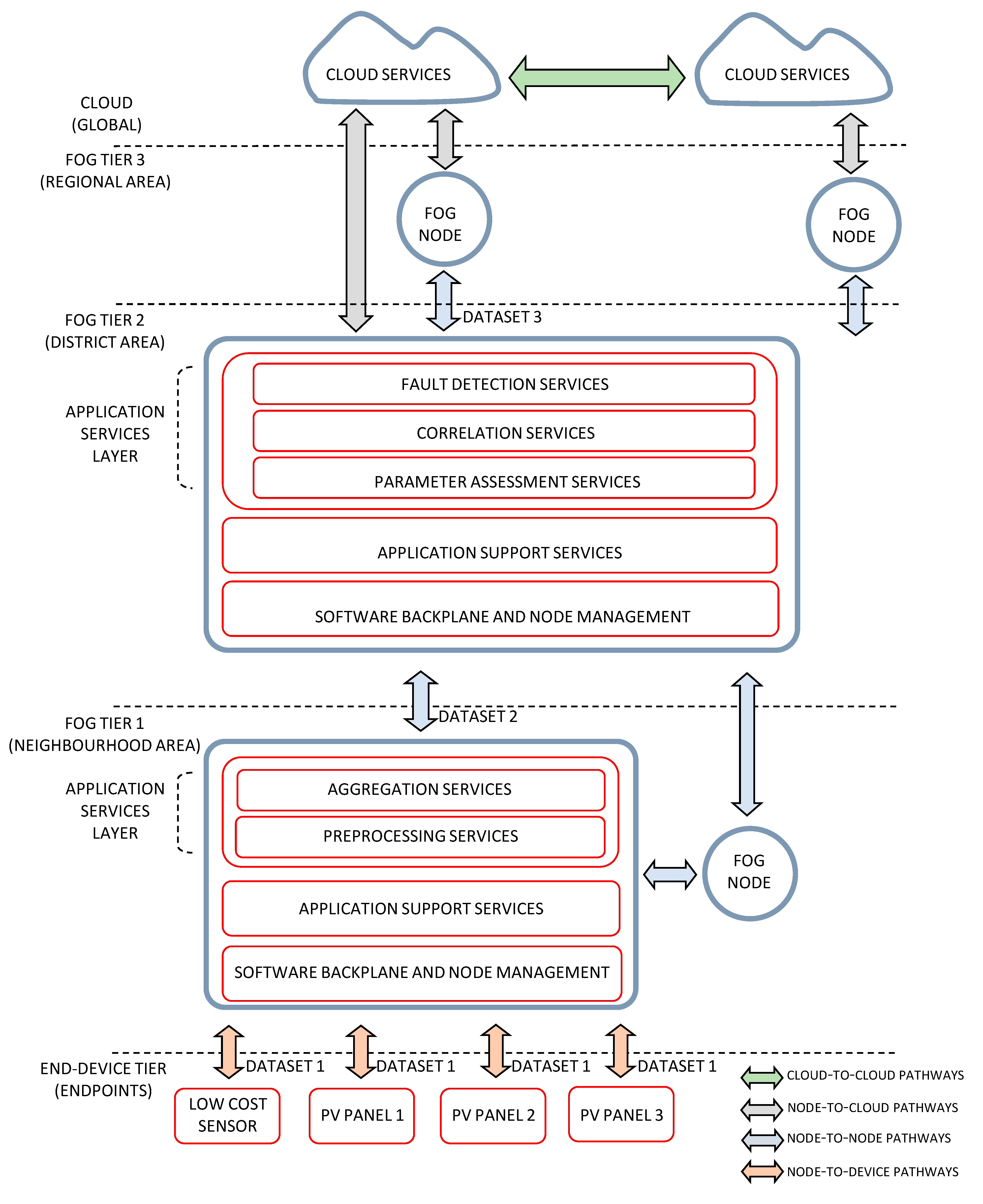
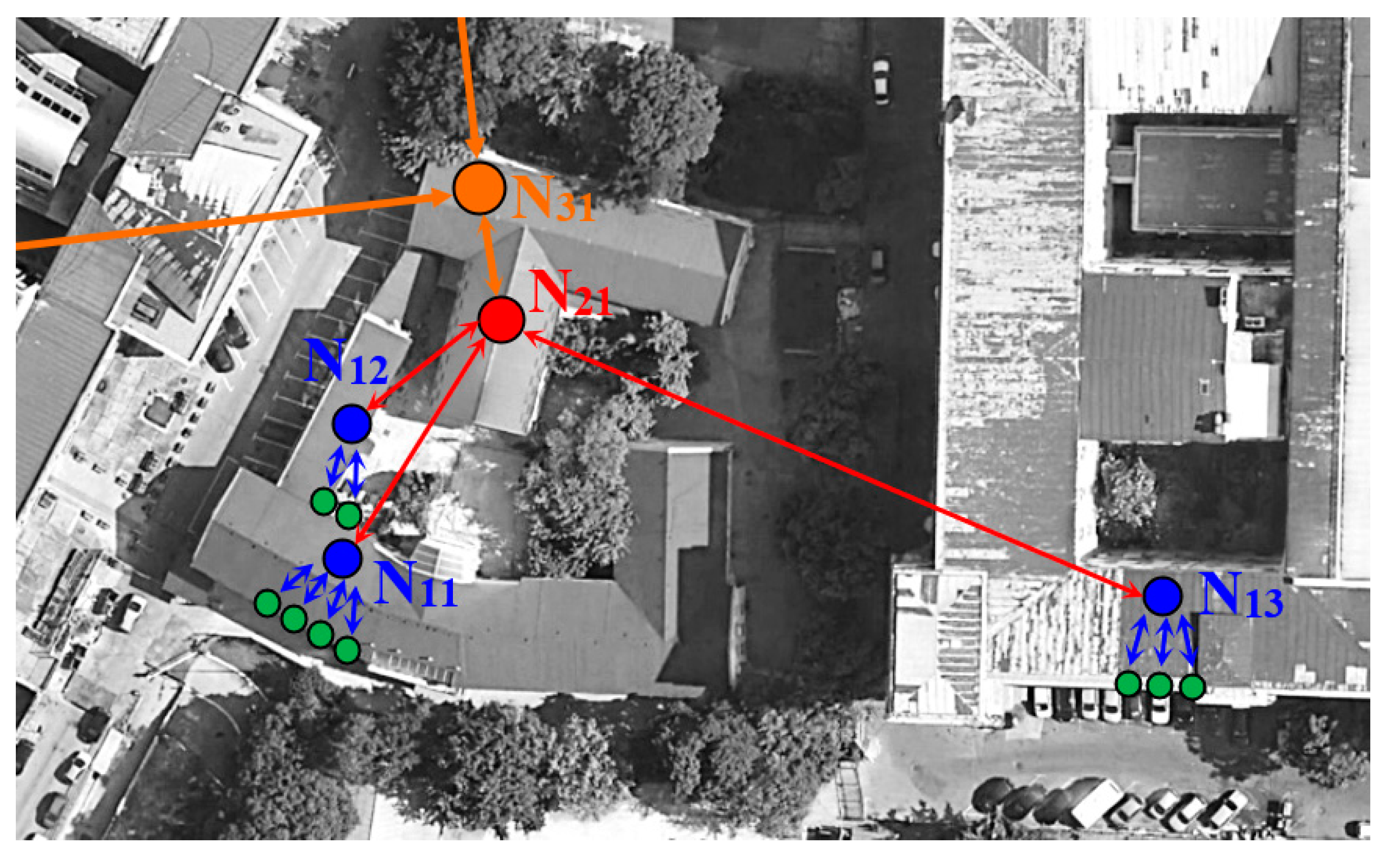
3.3. System Architecture and Service Deployment
4. Case Study
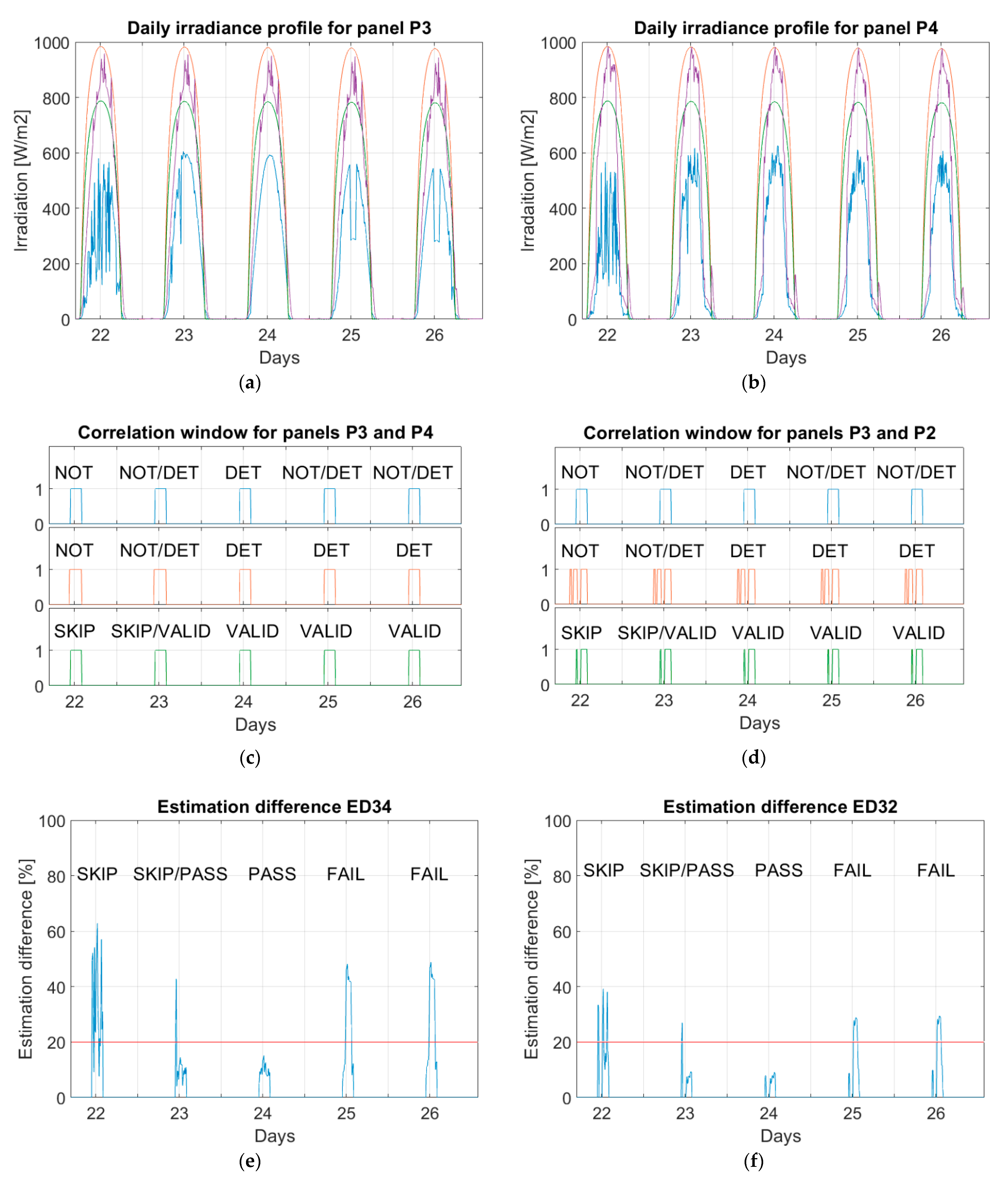
4.1. Detection of the On-Surface Degrading Effect
4.2. Detection of the Off-Surface Degrading Effect
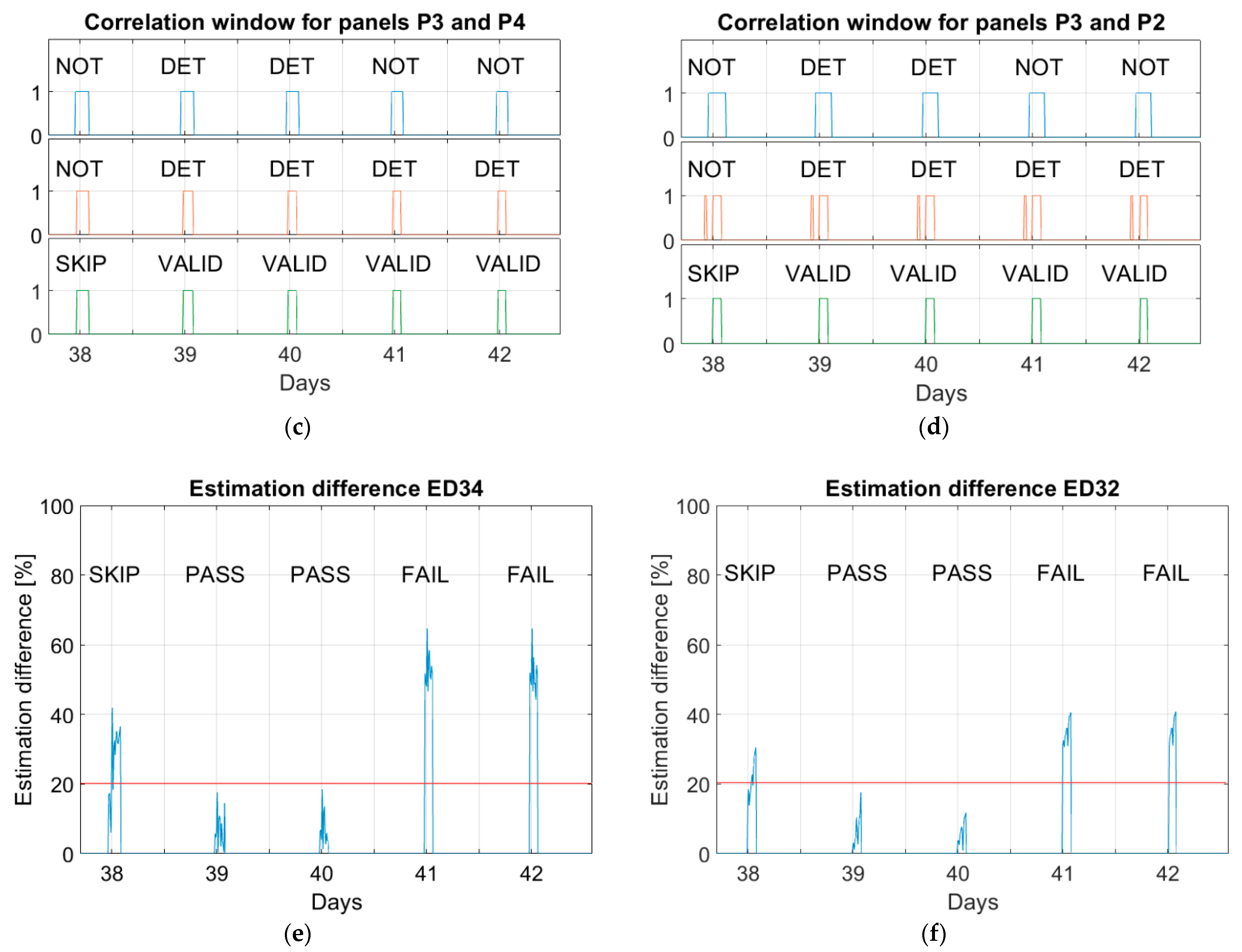
4.3. Detection of Soiling Degradation Effect
5. Conclusions
Author Contributions
Funding
Data Availability Statement
Acknowledgments
Conflicts of Interest
References
- IRENA. Future of Solar Photovoltaics-Deployment, Investment, Technology, Grid Integration and Socio-Economic Aspects; The International Renewable Energy Agency (IRENA): Abu Dhabi, United Arab Emirates, 2019. [Google Scholar]
- IRENA. Global Energy Transformation; The International Renewable Energy Agency (IRENA): Abu Dhabi, United Arab Emirates, 2018. [Google Scholar]
- Phillips, L.; Smith, P. Sustainable urban energy is the future. UN Chron. 2013, 52, 23–25. [Google Scholar] [CrossRef]
- Perea-Moreno, M.-A.; Hernandez-Escobedo, Q.; Perea-Moreno, A.-J. Renewable Energy in Urban Areas: Worldwide Research Trends. Energies 2018, 11, 577. [Google Scholar] [CrossRef]
- Livera, A.; Theristis, M.; Makrides, G.; Georghiou, G.E. Recent advances in failure diagnosis techniques based on performance data analysis for grid-connected photovoltaic systems. Renew. Energy 2019, 133, 126–143. [Google Scholar] [CrossRef]
- European Photovoltaic Industry Association; The Photovoltaic Technology Platform. Solar Europe Industry Initiative-Implementation Plan 2010–2012; EPIA: Bruxelles, Belgium, 2010. [Google Scholar]
- Stein, J.S. The photovoltaic Performance Modeling Collaborative (PVPMC). In Proceedings of the 2012 38th IEEE Photovoltaic Specialists Conference, Austin, TX, USA, 3–8 June 2012. [Google Scholar]
- Daliento, S.; Chouder, A.; Guerriero, P.; Pavan, A.M.; Mellit, A.; Moeini, R.; Tricoli, P. Monitoring, Diagnosis, and Power Forecasting for Photovoltaic Fields: A Review. Int. J. Photoenergy 2017, 2017, 1–13. [Google Scholar] [CrossRef]
- Theristis, M.; Venizelou, V.; Makrides, G.; Georghiou, G.E. Chapter II-1-B–Energy Yield in Photovoltaic Systems. In McEvoy’s Handbook of Photovoltaics, 3rd ed.; Kalogirou, S.A., Ed.; Academic Press: Cambridge, MA, USA, 2018; pp. 671–713. [Google Scholar]
- Benghanem, M. Low cost management for photovoltaic systems in isolated site with new IV characterization model proposed. Energy Convers. Manag. 2009, 50, 748–755. [Google Scholar] [CrossRef]
- Popovic, I.; Radovanovic, I. Methodology for detection of photovoltaic systems underperformance operation based on the correlation of irradiance estimates of neighbouring systems. J. Renew. Sustain. Energy 2018, 10, 053701. [Google Scholar] [CrossRef]
- Samikannu, S.M.; Namani, R.; Subramaniam, S.K. Power enhancement of partially shaded PV arrays through shade dispersion using magic square configuration. J. Renew. Sustain. Energy 2016, 8, 063503. [Google Scholar] [CrossRef]
- Hanson, A.J.; Deline, C.A.; MacAlpine, S.M.; Stauth, J.T.; Sullivan, C.R. Partial-Shading Assessment of Photovoltaic Installations via Module-Level Monitoring. IEEE J. Photovolt. 2014, 4, 1618–1624. [Google Scholar] [CrossRef]
- Leloux, J.; Narvarte, L.; Desportes, A.; Trebosc, D. Performance to Peers (P2P): A benchmark approach to fault detections applied to photovoltaic system fleets. Sol. Energy 2020, 202, 522–539. [Google Scholar] [CrossRef]
- Sathyanarayana, P.; Ballal, R.; Sagar, P.S.L.; Kumar, G. Effect of Shading on the Performance of Solar PV Panel. Energy Power 2015, 5, 1–4. [Google Scholar]
- Mani, M.; Pillai, R. Impact of dust on solar photovoltaic (PV) performance: Research status, challenges and recommendations. Renew. Sustain. Energy Rev. 2010, 14, 3124–3131. [Google Scholar] [CrossRef]
- Tatabhatla, V.M.R.; Agarwal, A.; Kanumuri, T. Enhanced performance metrics under shading conditions through experimental investigations. IET Renew. Power Gener. 2020, 14, 2592–2603. [Google Scholar] [CrossRef]
- Freire, F.; Melcher, S.; Hochgraf, C.G.; Kurinec, S.K. Degradation analysis of an operating PV module on a Farm Sanctuary. J. Renew. Sustain. Energy 2018, 10, 13505. [Google Scholar] [CrossRef]
- Madeti, S.R.; Singh, S. Monitoring system for photovoltaic plants: A review. Renew. Sustain. Energy Rev. 2017, 67, 1180–1207. [Google Scholar] [CrossRef]
- Mellit, A.; Tina, G.; Kalogirou, S. Fault detection and diagnosis methods for photovoltaic systems: A review. Renew. Sustain. Energy Rev. 2018, 91, 1–17. [Google Scholar] [CrossRef]
- Dhimish, M.; Holmes, V.; Dales, M. Parallel fault detection algorithm for grid-connected photovoltaic plants. Renew. Energy 2017, 113, 94–111. [Google Scholar] [CrossRef]
- Gallardo-Saavedra, S.; Hernández-Callejo, L.; Duque-Pérez, O. Quantitative failure rates and modes analysis in photovoltaic plants. Energy 2019, 183, 825–836. [Google Scholar] [CrossRef]
- Golnas, A.; Bryan, J.; Wimbrow, R.; Hansen, C.; Voss, S. Performance assessment without pyranometers: Predicting energy output based on historical correlation. In Proceedings of the 2011 37th IEEE Photovoltaic Specialists Conference, Washington, DC, USA, 19–24 June 2011. [Google Scholar]
- Elsinga, B.; Van Sark, W.G.J.H.M. Inter-system time lag due to clouds in an urban PV ensemble. In Proceedings of the 2014 IEEE 40th Photovoltaic Specialist Conference (PVSC), Denver, CO, USA, 8–13 June 2014. [Google Scholar]
- Engerer, N.; Mills, F. KPV: A clear-sky index for photovoltaics. Sol. Energy 2014, 105, 679–693. [Google Scholar] [CrossRef]
- Leloux, J.; Narvarte, L.; Trebosc, D. Review of the performance of residential PV systems in Belgium. Renew. Sustain. Energy Rev. 2012, 16, 178–184. [Google Scholar] [CrossRef]
- Lonij, V.P.A.; Jayadevan, V.T.; Brooks, A.E.; Rodriguez, J.J.; Koch, K.; Leuthold, M.; Cronin, A.D. Forecasts of PV power output using power measurements of 80 residential PV installs. In Proceedings of the 38th IEEE Photovoltaic Specialists Conference, Austin, TX, USA, 3–8 June 2012. [Google Scholar]
- Leloux, J.; Narvarte, L.; Luna, A.; Desportes, A. Automatic fault detection on BIPV systems without solar irradiation data. In Proceedings of the 29th European Photovoltaic Solar Energy Conference and Exhibition, Amsterdam, The Netherlands, 22–26 September 2014. [Google Scholar]
- Lonij, V.P.; Brooks, A.E.; Cronin, A.D.; Leuthold, M.; Koch, K. Intra-hour forecasts of solar power production using measurements from a network of irradiance sensors. Sol. Energy 2013, 97, 58–66. [Google Scholar] [CrossRef]
- Engerer, N.A. Estimating Collective Rooftop Photovoltaic Power Output; Australian Solar Council: Melbourne, Australia, 2012. [Google Scholar]
- Saint-Drenan, Y.M.; Good, G.H.; Braun, M.; Freisinger, T. Analysis of the uncertainty in the estimates of regional PV power generation evaluated with the upscaling method. Sol. Energy 2016, 135, 536–550. [Google Scholar] [CrossRef]
- Vergura, S. Hypothesis Tests-Based Analysis for Anomaly Detection in Photovoltaic Systems in the Absence of Environmental Parameters. Energies 2018, 11, 485. [Google Scholar] [CrossRef]
- Silvestre, S.; da Silva, M.A.; Chouder, A.; Guasch, D.; Karatepe, E. New procedure for fault detection in grid connected PV systems based on the evaluation of current and voltage indicators. Energy Convers. Manag. 2014, 86, 241–249. [Google Scholar] [CrossRef]
- Mayer, D.; Heidenreich, M. Performance analysis of stand alone PV systems from a rational use of energy point of view. In Proceedings of the 3rd World Conference on Photovoltaic Energy Conversion, Osaka, Japan, 11–18 May 2003. [Google Scholar]
- Dhimish, M.; Holmes, V.; Mehrdadi, B.; Dales, M. Diagnostic method for photovoltaic systems based on six layer detection algorithm. Electr. Power Syst. Res. 2017, 151, 26–39. [Google Scholar] [CrossRef]
- Mekki, H.; Mellit, A.; Salhi, H. Artificial neural network-based modelling and fault detection of partial shaded photovoltaic modules. Simul. Model. Prac. Theory 2016, 67, 1–13. [Google Scholar] [CrossRef]
- Vieira, R.G.; Dhimish, M.; De Araújo, F.M.U.; Guerra, M.I.S. PV Module Fault Detection Using Combined Artificial Neural Network and Sugeno Fuzzy Logic. Electronics 2020, 9, 2150. [Google Scholar] [CrossRef]
- Natsheh, E.; Samara, S. Tree Search Fuzzy NARX Neural Network Fault Detection Technique for PV Systems with IoT Support. Electronics 2020, 9, 1087. [Google Scholar] [CrossRef]
- Bertrand, C.; Housmans, C.; Leloux, J.; Journée, M. Solar irradiation from the energy production of residential PV systems. Renew. Energy 2018, 125, 306–318. [Google Scholar] [CrossRef]
- Saint-Drenan, Y.-M.; Bofinger, S.; Fritz, R.; Vogt, S.T.; Good, G.; Dobschinski, J. An empirical approach to parameterizing photovoltaic plants for power forecasting and simulation. Sol. Energy 2015, 120, 479–493. [Google Scholar] [CrossRef]
- Killinger, S.; Engerer, N.; Müller, B. QCPV: A quality control algorithm for distributed photovoltaic array power output. Sol. Energy 2017, 143, 120–131. [Google Scholar] [CrossRef]
- Kiefer, K.; Reich, N.H.; Dirnberger, D.; Reise, C. Quality assurance of large scale PV power plants. In Proceedings of the 2011 37th IEEE Photovoltaic Specialists Conference, Seattle, WA, USA, 19–24 June 2011. [Google Scholar] [CrossRef]
- Koch, S.; Weber, T.; Sobottka, C.; Fladung, A.; Clemens, P.; Berghold, J. Outdoor electroluminescence imaging of crystalline photovoltaic modules: Comparative study between manual ground-level inspections and drone-based aerial surveys. In Proceedings of the 32nd European Photovoltaic Solar Energy Conference and Exhibition, Munich, Germany, 20–24 June 2016. [Google Scholar]
- Kaplani, E. Detection of Degradation Effects in Field-Aged c-Si Solar Cells through IR Thermography and Digital Image Processing. Int. J. Photoenergy 2012, 2012, 1–11. [Google Scholar] [CrossRef]
- Tsanakas, J.A.; Ha, L.; Buerhop, C. Faults and infrared thermographic diagnosis in operating c-Si photovoltaic modules: A review of research and future challenges. Renew. Sustain. Energy Rev. 2016, 62, 695–709. [Google Scholar] [CrossRef]
- Fuentes, J.E.; Moya, F.D.; Montoya, O.D. Method for Estimating Solar Energy Potential Based on Photogrammetry from Unmanned Aerial Vehicles. Electronics 2020, 9, 2144. [Google Scholar] [CrossRef]
- Mohammed, Y.; Mustafa, M.; Bashir, N.; Mokhtar, A. Renewable energy resources for distributed power generation in Nigeria: A review of the potential. Renew. Sustain. Energy Rev. 2013, 22, 257–268. [Google Scholar] [CrossRef]
- Oyedepo, S.O. Towards achieving energy for sustainable development in Nigeria. Renew. Sustain. Energy Rev. 2014, 34, 255–272. [Google Scholar] [CrossRef]
- Aliyu, A.K.; Modu, B.; Tan, C.W. A review of renewable energy development in Africa: A focus in South Africa, Egypt and Nigeria. Renew. Sustain. Energy Rev. 2018, 81, 2502–2518. [Google Scholar] [CrossRef]
- Aliyu, A.S.; Dada, J.O.; Adam, I.K. Current status and future prospects of renewable energy in Nigeria. Renew. Sustain. Energy Rev. 2015, 48, 336–346. [Google Scholar] [CrossRef]
- Giwa, A.; Alabi, A.; Yusuf, A.; Olukan, T. A comprehensive review on biomass and solar energy for sustainable energy generation in Nigeria. Renew. Sustain. Energy Rev. 2017, 69, 620–641. [Google Scholar] [CrossRef]
- Akuru, U.B.; Onukwube, I.E.; Okoro, O.I.; Obe, E.S. Towards 100% renewable energy in Nigeria. Renew. Sustain. Energy Rev. 2017, 71, 943–953. [Google Scholar] [CrossRef]
- Ohunakin, O.S.; Adaramola, M.S.; Oyewola, O.M.; Fagbenle, R.O. Solar energy applications and development in Nigeria: Drivers and barriers. Renew. Sustain. Energy Rev. 2014, 32, 294–301. [Google Scholar] [CrossRef]
- Okoye, C.O.; Taylan, O.; Baker, D.K. Solar energy potentials in strategically located cities in Nigeria: Review, resource assessment and PV system design. Renew. Sustain. Energy Rev. 2016, 55, 550–566. [Google Scholar] [CrossRef]
- Soshinskaya, M.; Crijns-Graus, W.H.; Guerrero, J.M.; Vasquez, J.C. Microgrids: Experiences, barriers and success factors. Renew. Sustain. Energy Rev. 2014, 40, 659–672. [Google Scholar] [CrossRef]
- Wang, H.; Peng, Y.; Yang, Z. Analyzing the key technologies of large-scale application of PV grid-connected systems. In Proceedings of the 2010 International Conference on Power System Technology, Hangzhou, China, 24–28 October 2010. [Google Scholar]
- Akinyele, D.; Belikov, J.; Levron, Y. Challenges of Microgrids in Remote Communities: A STEEP Model Application. Energies 2018, 11, 432. [Google Scholar] [CrossRef]
- Wu, H.; Hou, Y. Recent Development of Grid-Connected PV Systems in China. Energy Procedia 2011, 12, 462–470. [Google Scholar] [CrossRef]
- Aazam, M.; Huh, E.-N. Fog computing: The cloud-iot/ioe middleware paradigm. IEEE Potentials 2016, 35, 40–44. [Google Scholar] [CrossRef]
- OpenFog Consortium Architecture Working Group. OpenFog Reference Architecture for Fog Computing OpenFog Consortium. OPFRA001 2017, 20817, 162. [Google Scholar]
- Radovanovic, I.; Popovic, I.; Drajic, D. Multi channel sensor measurements in fog computing architecture. In Proceedings of the 2017 Zooming Innovation in Consumer Electronics International Conference (ZINC), Novi Sad, Serbia, 31 May–1 June 2017. [Google Scholar]
- American Society of Heating, Refrigeration, and Air-Conditioning Engineers. ASHRAE Handbook: Fundamentals; ASHRAE: Atlanta, GA, USA, 2001. [Google Scholar]


| Type of Analysis | Reference | Advantages | Disadvantages |
|---|---|---|---|
| Cross-correlation analysis with environmental sensing | [11,24,25,26,27,28,29,30] | Real-time fault detection and identification/automatic fault detection Applicable to distributed energy resources (DER) Low processing requirements Low hardware requirements Performance quantification | Highly sensitive to meteorological conditions Limited fault type identification Inability to identify multiple faults |
| Performance analysis without environmental sensing | [14,21,28,32] | Automatic fault detection Applicable to PV fields Low processing requirements Low hardware requirements Performance quantification | Limited applicability to DER Limited fault type identification Inability to identify multiple faults |
| Reference-model-based analysis | [31,33,34] | Real-time automatic fault detection Low processing requirements Low hardware requirements Performance quantification | Highly sensitive to meteorological conditions Limited applicability to DER Limited fault identification Sensitive to the variations of model parameters |
| Methods based on artificial intelligence techniques | [35,36,37,38] | Ability to diagnose multiple faults Near-real-time detection Performance quantification | Periodical model training required Sensitive to the variations of model parameters Highly limited applicability to DER High processing requirements High hardware requirements Time-consuming |
| Methods based on imaging techniques | [43,44,45,46] | Capability for comprehensive fault diagnosis Ability to diagnose multiple faults Physical fault inspection | High processing requirements High hardware requirements Highly limited applicability to DER No performance quantification Time consuming |
| PV Panel | Type | Characteristics | Orientation | Installation |
|---|---|---|---|---|
| P1 and P2 | Solar fabrik (Polycrystalline silicon) | surface area A = 1.522 m2 module efficiency ηr = 17.14% at 25 °C temperature coefficient βTC = −0.43%/°C maximum power PM = 280 W | tilt angle β = 36° azimuth angle γ = 180° | Telefon Inzenjering M1000/12 battery backup |
| P3 | Renewsys Deserv (Polycrystalline silicon) | surface area A = 1.013 m2 module efficiency ηr = 14.80% at 25°C. temperature coefficient βTC = −0.5%/°C maximum power PM = 150 W | tilt angle β = 26° azimuth angle γ = 180° | MEAN WELL TS-1500 battery backup |
| P4 and P5 | Sun Spark SMX-250P (Polycrystalline silicon) | surface area A = 1.645 m2 module efficiency ηr = 15.20% at 25 °C, temperature coefficient βTC = −0.4%/°C maximum power PM = 250 W | tilt angle β = 32° azimuth angle γ = 180° | MEAN WELL TS-1500 battery backup |
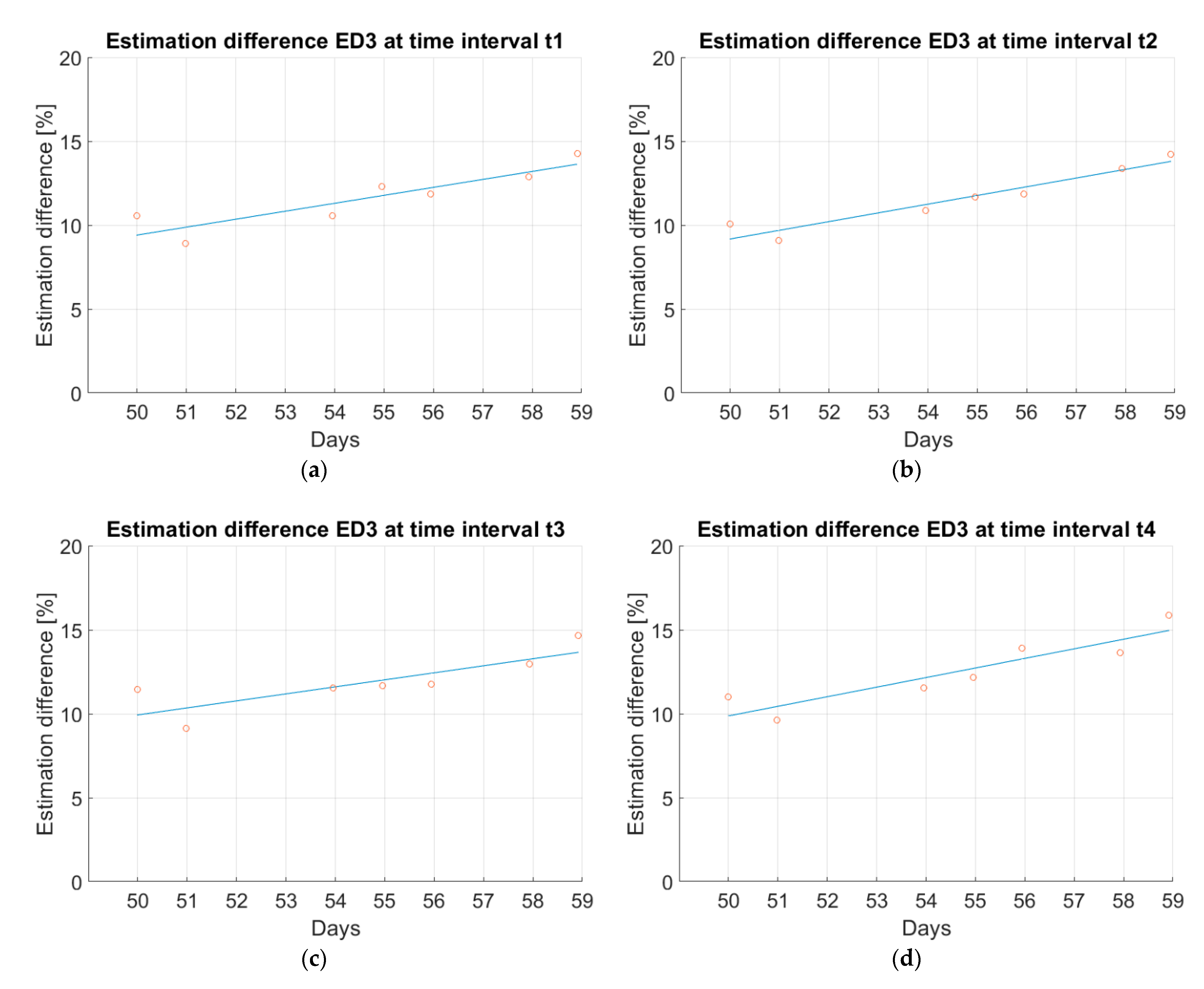
| Period | STATUS | Slope [%/day] | |||||||||
|---|---|---|---|---|---|---|---|---|---|---|---|
| t1 | DET | DET | NOT | NOT | DET | DET | DET | NOT | DET | DET | 0.41 |
| t2 | DET | DET | NOT | NOT | DET | DET | DET | NOT | DET | DET | 0.43 |
| t3 | DET | DET | NOT | NOT | DET | DET | DET | NOT | DET | DET | 0.37 |
| t4 | DET | DET | NOT | NOT | DET | DET | DET | NOT | DET | DET | 0.49 |
| Days | 50 | 51 | 52 | 53 | 54 | 55 | 56 | 57 | 58 | 59 | |
Publisher’s Note: MDPI stays neutral with regard to jurisdictional claims in published maps and institutional affiliations. |
© 2021 by the authors. Licensee MDPI, Basel, Switzerland. This article is an open access article distributed under the terms and conditions of the Creative Commons Attribution (CC BY) license (http://creativecommons.org/licenses/by/4.0/).
Share and Cite
Radovanovic, I.; Popovic, I. Identification of Degrading Effects in the Operation of Neighboring Photovoltaic Systems in Urban Environments. Electronics 2021, 10, 762. https://doi.org/10.3390/electronics10070762
Radovanovic I, Popovic I. Identification of Degrading Effects in the Operation of Neighboring Photovoltaic Systems in Urban Environments. Electronics. 2021; 10(7):762. https://doi.org/10.3390/electronics10070762
Chicago/Turabian StyleRadovanovic, Ilija, and Ivan Popovic. 2021. "Identification of Degrading Effects in the Operation of Neighboring Photovoltaic Systems in Urban Environments" Electronics 10, no. 7: 762. https://doi.org/10.3390/electronics10070762
APA StyleRadovanovic, I., & Popovic, I. (2021). Identification of Degrading Effects in the Operation of Neighboring Photovoltaic Systems in Urban Environments. Electronics, 10(7), 762. https://doi.org/10.3390/electronics10070762