A Hybrid YOLOv4 and Particle Filter Based Robotic Arm Grabbing System in Nonlinear and Non-Gaussian Environment

Abstract

In this paper, we propose a robotic arm grasping system suitable for complex environments. For a robotic arm, in order to achieve its accurate grasp of the target object, not only the vision but also a certain tracking ability should be provided. To improve the grasp quality, we propose a robotic arm grasping system using YOLOv4 combined with a particle filter (PF) algorithm, which can be applied in a nonlinear and non-Gaussian environment. Firstly, the coordinates of the bounding box in the image can be obtained through the YOLOv4 object detection algorithm. Secondly, the coordinates in the world system can be obtained through the eye-to-hand calibration system. Thirdly, a PF model can be established based on the coordinate changes of the target object. Finally, according to the predicted output of the PF, the robotic arm and the target object can reach the specific position at the same time and complete the grab. As the target object, the bowl is applied to experiments for the sake of achieving a more convincing demonstration. The experimental results show that the robotic arm grasping system proposed in this paper can accomplish the successful grasp at a rate of nearly 88%, even at a higher movement speed, which is of great significance to robot applications in various fields.

1. Introduction

The fourth industrial revolution will lead to disruptive changes in the industry [1]. The integration and development of information technology and control theory have made robots an essential part of modern industrial production [2]. With the rapid development of machine vision, robotic arms can automatically recognize different kinds of objects [3,4]. Tracking and capturing them has greatly improved human production efficiency which brings rapid development in the field of human technology. Additionally, many other industries gradually replace manpower with robots. For example, in the catering industry, the investment of robots has made the catering industry more hygienic. In this paper, research on automatic recognition and target object grabbing will be carried out.

There are generally two ways to achieve the grasp of the robotic arm. One is to grasp by teaching [5]. On the basis of the preset path, the robotic arm can do a repeating movement to realize automated production. However, in this method, a disturbance can be easily caused by the environment. The change of links will result in the stagnation of all production. The other is to combine machine learning or deep learning to achieve a more intelligent grasp and better completion. Accordingly, a combination of identification and tracking [6,7] is highly required. As we all know, people are able to recognize the type and location of objects at first glance. It is easy for us to understand how they interact [8]. However, it is hard for machine vision to achieve such an effect. Therefore, precise recognition of the target object is fundamental to a successful grasp. There are two ways to identify. One is the traditional detection algorithm, and the other is the detection algorithm combined with deep learning. Yonghao Zhao et al. [9] adopted Canny operator edge detection by utilizing binocular three-dimensional vision to obtain the robotic arm grab point. The PID (proportion integral differential) position algorithm was used to track the object dynamically. Honglei Wei et al. [10] used the Canny operator in the video image sequence to detect the edge of the target and the mean-shift algorithm was used to realize the target localization and tracking. It is easy to use the detecting methods that adopt the Canny operator. It can mark the edges of the target object as much as possible, but its disadvantage is that the existing image noise may also be marked as edges. Moreover, the light intensity of the environment [11] and the change of target feature will interfere with the position of the target object obtained in the image. By comparison, the object detection algorithm based on deep learning shows better robustness in detecting. “You only look once (YOLO)”, which is created to achieve the purpose, will recognize what and where the target object is in just one sight. It converts the object detection framework into a bounding box for spatial segmentation and regression of related probabilities. In an evaluation, a single neural network directly predicts the bounding box and class probability from the complete image. Furthermore, the detection efficiency of YOLO is very fast [12], which can meet the visual requirements of robotic arm recognition and capture. Unlike the current detection algorithms commonly used in the industry, such as SSD [13], Mask R-CNN [14], and Cascade R-CNN [15], the study demonstrates that YOLO achieves high detection accuracy and at the same time maintains high FPS (frames per second). Shehan P Rajendran et al. [16] proposed that using YOLOv3 to recognize road signs shows high real-time performance and accuracy when compared with Faster R-CNN. Jinmin Peng et al. [17] used the idea of hollow convolution in YOLOv3 so that the average detection accuracy of the workpiece reached 92.98%. However, the latest research on YOLOv4 shows better results in detection [18]. As for YOLOv5, the model frameworks of YOLOv5 and YOLOv4 are basically the same, but YOLOv4 is more customizable, and with the addition of more custom configuration conditions, YOLOv4 is still the best object detection framework. Consequently, in this paper, how to apply deep learning to identify the target will be discussed. More importantly, the significance and innovation of using YOLOv4 to identify the target are illustrated in this paper.

In addition to object recognition, tracking is also indispensable for the robotic arm to make a precise grasp [6]. In order to provide the robotic arm with the position of the next moment, the current measurement, the observation measurement, and the system model in the dynamic system should be known [19]. The tracking based on the target motion model can be roughly divided into three categories, namely tracking based on PID, kernel methods, and filtering theory. The PID-based tracking algorithm is shown by Yonghao Zhao et al. [9], and its advantage is simple and fast. However, it is essential to constantly adjust the PID gain in an environment full of random disturbances. Otherwise, it will not make an excellent performance. The main tracking method based on the kernel method is the mean-shift. As shown by Honglei Wei et al. [10], it has a small amount of calculation and high real-time performance, but it often fails when tracking small targets and fast-moving targets, which cannot be ignored in a stable grasping system. The tracking methods based on filter theory include the Kalman filter (KF) algorithm and the PF algorithm. Hitesh A Patel et al. [20] used KF to track a single moving object. Shiuh-Ku Weng et al. [21] proposed adaptive KF which has a better performance in tracking. However, most of them are used for a linear system. If the environment changes unpredictably, that is, the system produces nonlinear motion, their performance won’t be satisfactory. In contrast, in nonlinear and non-Gaussian systems, PF performs better in tracking and predicting. M. Sanjeev Arulampalam et al. [22] conducted analysis and investigation experiments on KF, extended KF, and PF, which confirmed the performance of PF in the nonlinear and non-Gaussian environment. Junlan Yang et al. [23] used PF to estimate and track target objects in video sequences and concluded that increasing the number of particles can reduce the estimated variance of the time series and make the estimated value smoother and more accurate. Therefore, in a non-linear environment, the PF algorithm is more robust than the KF algorithm [24]. The second aspect of significance and innovation in using the PF method to track and predict the target will be illustrated as well, which could reduce environmental interference.

On this basis, due to the complicated and changeable catering environment, we propose to use YOLOv4 with the PF algorithm to dynamically grab the moving target in the nonlinear and non-Gaussian environment.

The main contributions of this paper can be summarized as follows:

(1)

In this paper, the most widely used contemporary YOLO algorithm is analyzed theoretically and compared with other algorithms. In addition, three distances and FPS are tested using the latest YOLOv4 algorithm as well as commonly used detection algorithms to achieve efficient detection of YOLOv4 in real-time. The average recognition accuracy reaches 98.5% and the FPS is maintained at around 22 FPS.

(2)

The laboratory tests on different filters with filtering and prediction functions are run under simulated situations in this paper. With the existence of environmental interference, the exquisite filtering and prediction functions of the PF algorithm are fulfilled. Its MSE of the filter error is 7.1537 × 10⁻⁶ and its MSE of the prediction error is 1.356 × 10⁻⁵, indicating that it can effectively reduce the impact of the environment to get the predicted position of the target object at the next moment more accurately.

(3)

In this paper, we use a grabbing system that combines YOLOv4 and PF algorithms to conduct a large number of comparative experiments. YOLOv4 can maintain an accuracy of nearly 99.50% while recognizing the object from a proper distance. Additionally, its recognition speed meets the requirements of real-time and the ability of PF to adjust the sudden disturbances is also significantly higher than that of other filter algorithms such as KF. Therefore, the grabbing system can accomplish the successful grasp at a rate of nearly 88% even at a higher movement speed.

Our work is structured as follows: in Section 2, the robotic arm grabbing system is preliminarily presented. In Section 3, the YOLOv4 algorithm is used to identify and obtain the position of the target object in the image. In Section 4, the PF is used to obtain the transition matrix and observation matrix of the target object’s motion and predict the motion state of the target object at the next moment. In Section 5, through a large number of comparative simulation experiments and tests in a real environment, the PF is shown to affirm its excellent tracking and prediction performance in a nonlinear and non-Gaussian environment. In Section 6, the research of the whole paper is summarized.

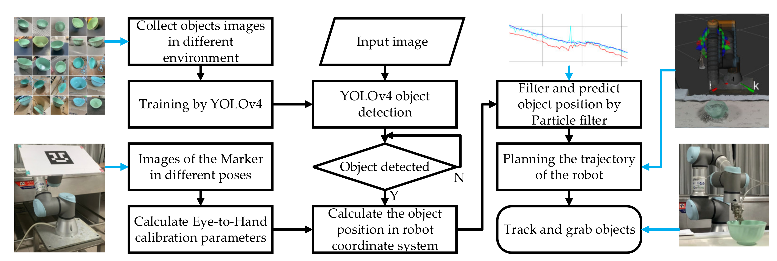
2. Framework of Moving Target Tracking and Grabbing Strategy

The following are the characteristics of moving target tracking, predicting, and grabbing in real life. Firstly, the image of the target object collected by the RGB-D sensor may be deformed, which may cause the center point of the target to drift. Secondly, the conveyor belt environment may be disturbed by its own or external influences, causing objects on the conveyor belt to become non-linear motions, resulting in failing grasps. Thirdly, the image sensor sampling rate and image processing rate are much lower than the system control cycle, which will lead to a delay in tracking.

Considering the above characteristics, we proposes a robotic grabbing system that can be used in a nonlinear non-Gaussian environment, with the combination of the YOLOv4 object detection algorithm and PF tracking algorithm. The framework of the robotic arm grabbing system is shown in Figure 1. Before detecting the target object, its images should be collected in a different environment, and then it will be trained by YOLOv4. Then, by calculating the relative position of the RGB-D sensor and the robotic arm through different positions of the marker board, we can obtain the eye-to-hand calibration parameter. When the target object is detected, we can clarify its real coordinate points. By passing these coordinate points through PF, the most likely position of the target object at the next moment can be obtained. Finally, following the planned trajectory, the robotic arm reaches the grasping position to grasp the target.

3. Target Recognition Based on YOLOv4 Algorithm

Object detection is one of the important components of deep learning in the field of computer vision. Its task is to find all objects of interest in the image, including two subtasks: object location and object classification, and determine the category and location of the object at the same time. Object detection can be divided into two categories: one is based on Region Proposal’s R-CNN series of algorithms (R-CNN, Fast R-CNN, Faster R-CNN, etc.). They are two-stage algorithms and firstly need to be used to generate object candidate boxes which will then be classified and regressed. The other are YOLO series and SSD series, the one-stage algorithms, which use a convolutional neural network to simultaneously predict the target category and position. The two-stage algorithm has higher recognition accuracy, but its real-time performance is poor, while the one-stage algorithm is faster in speed but slightly lower in accuracy [25]. However, starting from YOLOv3, the YOLO series achieves a better trade-off between recognition accuracy and speed, and YOLOv4 uses CIoU loss as the loss of the bounding box, which can converge faster and have better performance [18]. Due to the requirements of real-time and accuracy, we propose to use a one-stage algorithm YOLOv4 to realize the task of identifying the bowl on the conveyor belt.

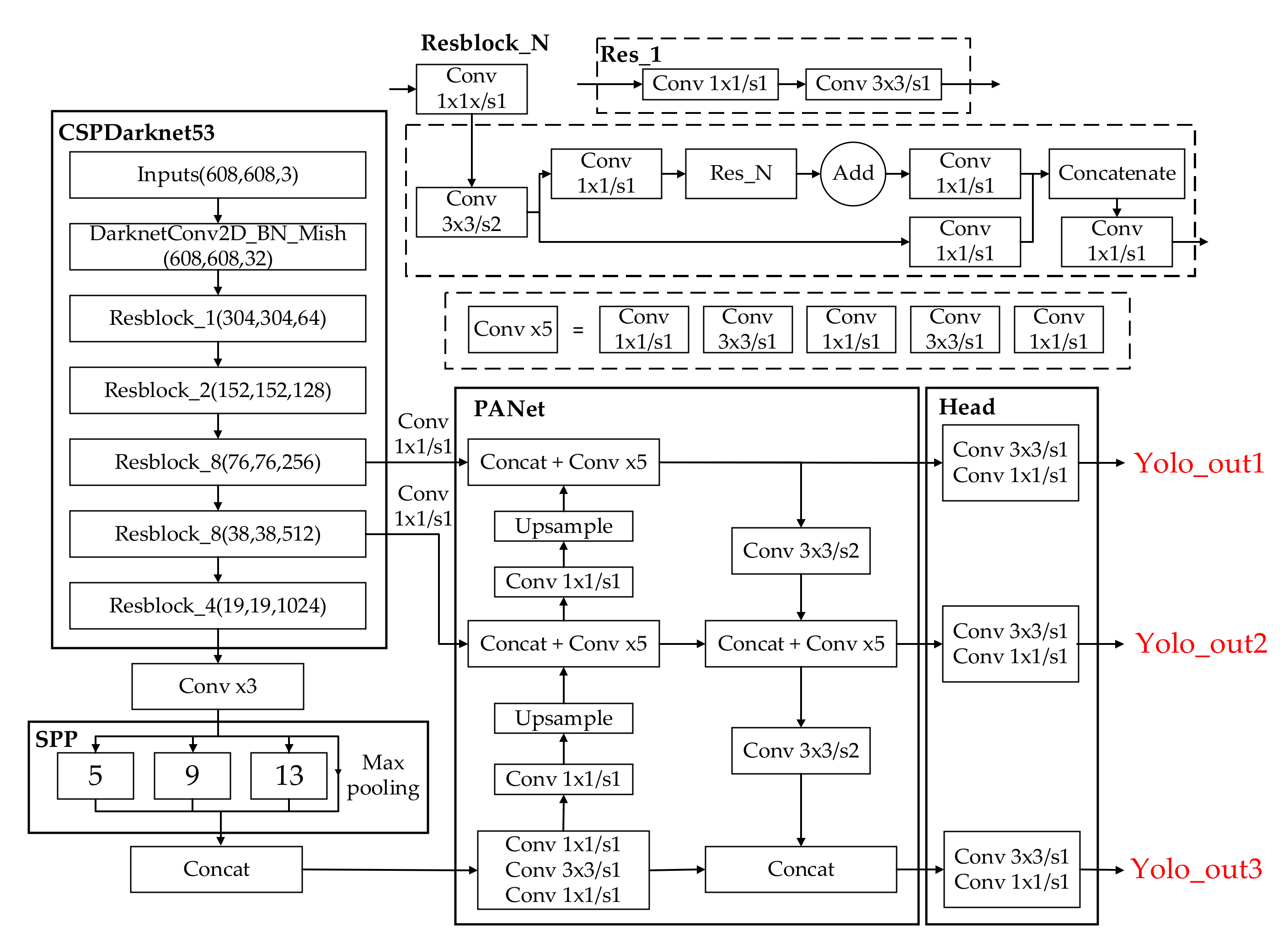
3.1. YOLOv4 Algorithm Structure

YOLOv3 is an end-to-end object detection algorithm whose model structure mainly consists of the Darknet-53 backbone network (Backbone) and multi-scale fusion feature network (FPN) [26,27]. The backbone network Darknet-53 is primarily used to extract image features. The network is mainly composed of five residual blocks, and each residual block contains a set of repeated residual units. The connection of a Batch Normalization (BN) layer and a Leaky ReLU activation function is after each convolutional layer, namely the Con2d layer. Based on the original YOLO object detection architecture, YOLOv4 retains the head of YOLOv3 and uses a more powerful backbone network CSPDarknet53. Additionally, it uses the idea of spatial pyramid pooling (SPP) to expand the receptive field and chooses PANet as the Neck part for feature fusion as shown in Figure 2. Meanwhile, it can be improved and optimized due to the use of the Mish activation function, Mosaic data enhancement, and DropBlock regularization.

Integrating CSP on each large residual block of Darknet53, CSPDarknet53 can enhance the learning ability of CNN and maintain accuracy while the weight, computing bottlenecks, and memory costs are reduced. The input before each large residual block (Resblock) is divided into two parts, one of which is input to the stacked residual unit, and the other is directly convolved. Then the results of the two parts are concatenated, and finally output through convolution.

To expand the receptive field of the network, an SPP network needs to be added after Backbone. First, the output of the feature extraction network is subjected to three convolution operations and maximized through the pooling of 1 × 1, 5 × 5, 9 × 9, and 13 × 13. Then the four pooled outputs are concatenated into a feature map, and finally convolution dimensionality reduction can be done.

The Neck part of object detection is mainly used to fuse the feature information of feature maps of different sizes. YOLOv4 uses the feature fusion method of PANet. Based on the top-down feature fusion of FPN, the bottom-up feature fusion is added to shorten the information for the dissemination path which uses low-level features to accurately locate information. Additionally, each proposal can use the features of all layers of the pyramid if the method of dynamic feature pooling is used. After feature fusion, the network will output three different sizes of feature maps, 19 × 19 (Yolo_out1), 38 × 38 (Yolo_out2), 76 × 76 (Yolo_out3), corresponding to the prediction of large, medium, and small scale objects respectively.

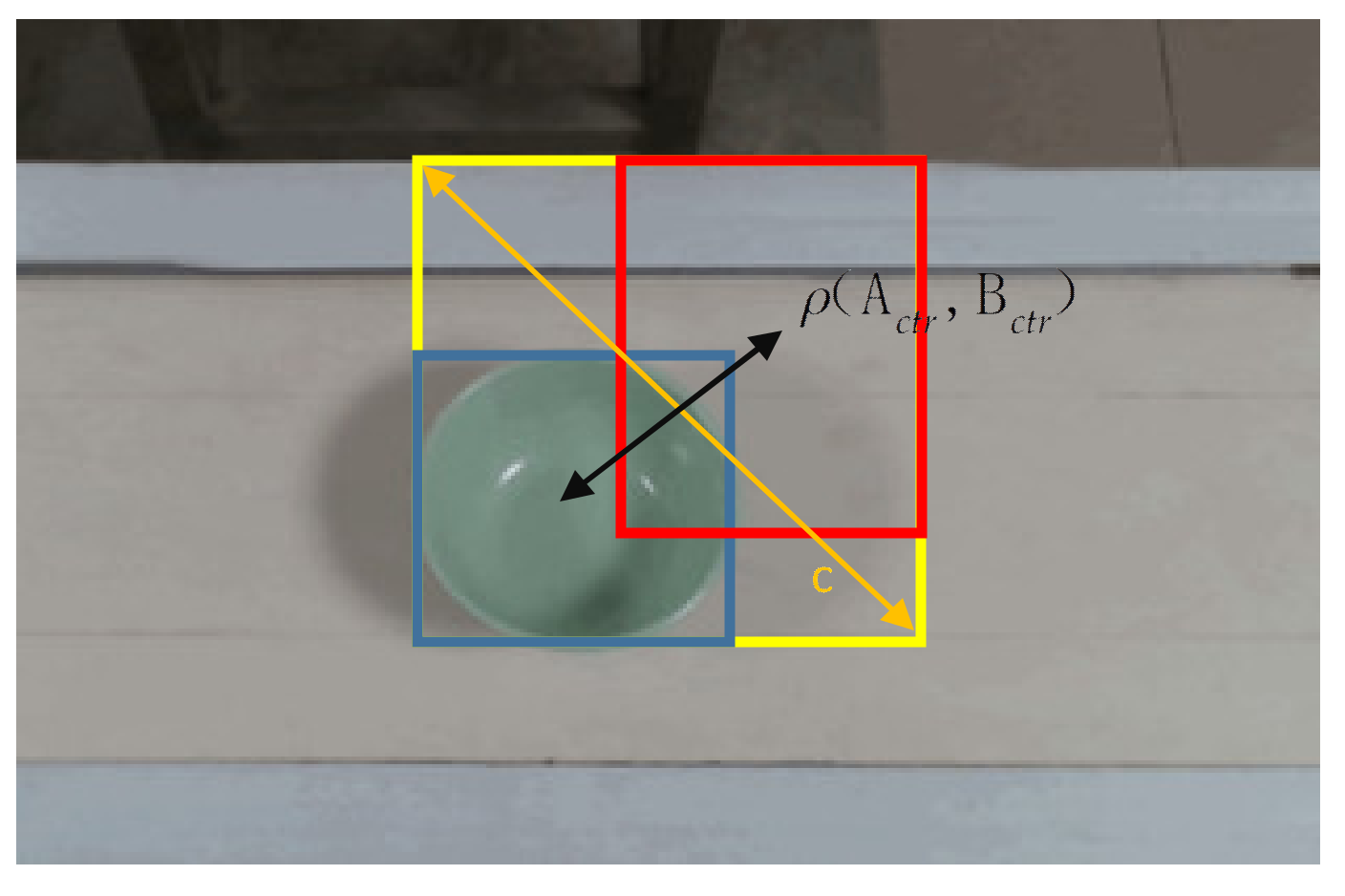
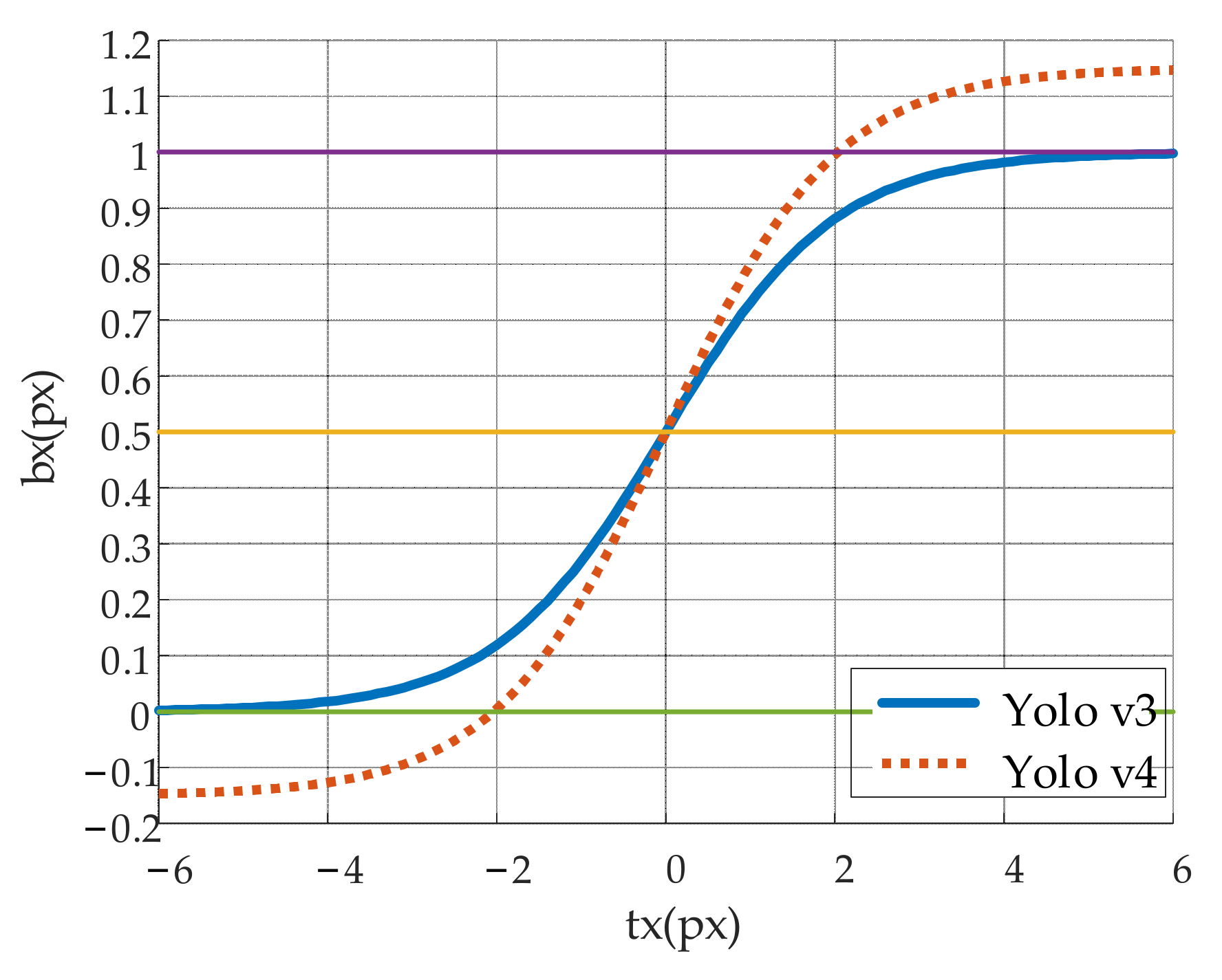
3.2. The Loss of YOLOv4

YOLOv3 uses MSE (mean square error) directly based on the coordinates of the center point of the prediction box and the real box as well as the width and height information. However, the MSE loss function fails to reflect the relationship between the information, but uses it as an independent variable. In order to improve it, IoU loss is proposed, which considers the area of the predicted bounding box (BBOX) and the ground truth bounding box [28,29]. YOLOv4 uses CIoU loss instead of MSE loss, which includes the shape and direction of the object and also considers the overlap area, the distance between the center points, and the aspect ratio, which are defined as follows.

$$L_{CIoU}=1-IoU(A,B)+{\rho }^2(A_{ctr},B_{ctr})/c^2+\alpha ·\lambda$$

(1)

$$IoU(A,B)=\frac{area(A\cap B)}{area(A\cup B)}$$

(2)

$$\alpha =\frac{\lambda }{(1-IoU(A,B))+\lambda }$$

(3)

$$\lambda =\frac{4}{{\pi }^2}{(\arctan \frac{w^{gt}}{h^{gt}}-\arctan \frac{w}{h})}^2$$

(4)

A represents the prediction frame. B represents the real frame. ρ (A_ctr,B_ctr)/c² represents the penalty for the center point distance. A_ctr represents the center point coordinates of the prediction frame. B_ctr represents the center point coordinates of the real frame. ρ(·) represents the Euclidean distance, and C represents the distance between A and B as shown in Figure 3. α·λ represents the penalty for the aspect ratio. α is a positive coefficient, and λ is used to measure the consistency of the aspect ratio. gt means ground truth. w^gt and h^gt are the width and height of the real frame. w and h are the width and height of the prediction frame. If the width and height of the real frame and the prediction frame are similar, then λ tends to 0, and the penalty is invalid. Intuitively, the penalty term is used to control the width and height of the predicted frame to move toward the width and height of the real frame as soon as possible.

$$L_{ciou}=Pr\left(object\right)·L_{CIoU}$$

(5)

$$L_{prob}=Pr\left(object\right)·L_{SCE}\left(y,p\right)$$

(6)

$$L_{conf}=Pr\left(object\right)·L_{BCE}\left(y,p\right)+\left(1-Pr\left(object\right)\right)*L_{BCE}\left(y,p\right)*IgnoreMask$$

(7)

$${\lambda }_{ciou}=2-\left(\frac{w^{gt}·h^{gt}}{w·h}\right)$$

(8)

$$Loss={\lambda }_{ciou}·L_{ciou}+L_{prob}+L_{conf}$$

(9)

In the above equation, λ_ciou plays a role in balancing the loss. It is used to increase the weight of the position loss of the bounding box and suppress the bounding box confidence of undetected objects. L_SCE means sigmoid cross entropy. L_BCE means binary cross entropy. y means real value. p means predicted value. If the center point of the real frame belongs to the prediction frame, it is assumed that the prediction frame has a target. Then Pr(object) = 1, if not, Pr(object) = 0. IgnoreMask means when there is no target, the IoU of the prediction frame and the real frame are calculated, and the largest IoU is selected as the IoU of the predicted and the real value. An IoU threshold is set, and when its maximum IoU is less than this threshold, it will be added to the loss function calculation as Equation (7). L_ciou means location loss. L_prob means class loss. L_conf means confidence loss. Then we could obtain the loss of YOLOv4 through Equation (9).

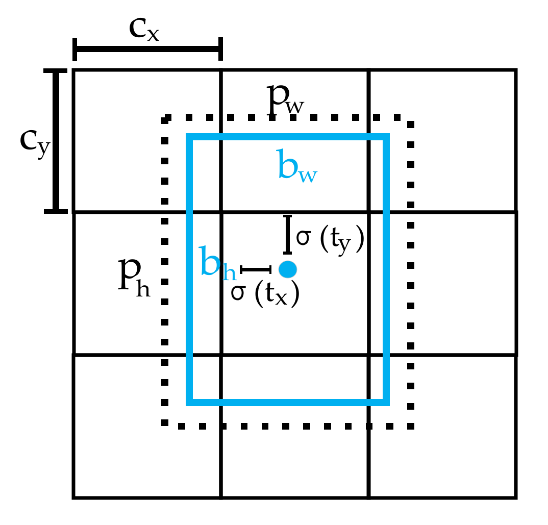
3.3. Target Position Coordinate Calculation

When it is confirmed that the target object is detected, we can extract the position of the target object in the image, as shown in Figure 4. The box consisting of dots in Figure 4 is the anchor. In the anchor-based target detection algorithm, it is generally designed manually by designing nine anchors with different sizes and aspect ratios. One disadvantage of the manually designed anchors is that they are not guaranteed to fit the dataset well. If the size of the anchor differs significantly from that of the target, the detection effect of the model will be affected. In YOLO, we use the k-means clustering algorithm instead of a manual design to generate the anchors that fit the dataset by clustering the bounding box of the training set to improve the detection effect of the network. c_x and c_y represent the coordinates of the upper left corner of the area where the center point is located. p_w and p_h represent the width and height of the anchor, respectively. σ(t_x) and σ(t_y) represent the distance between the center point of the prediction box and the upper left corner respectively, and σ represents the sigmoid function, which limits the offset to the current grid and is conducive to model convergence.

The calculation Equation (10) for the actual position and size of the target object in YOLOv3 is:

$$\begin{array}{l}{b}_{x\_YOLOv3}=\sigma (t_x)+c_x\\ b_{y\_YOLOv3}=\sigma (t_y)+c_y\\ b_{w\_YOLOv3}=p_w{e}^{tw}\\ b_{h\_YOLOv3}=p_h{e}^{th}\end{array}$$

(10)

t_w and t_h represent the predicted width and height offset. The length and width of the anchor are adjusted. b_{x_YOLOv3} and b_{y_YOLOv3} can obtain the position of the target object. b_{w_YOLOv3} and b_{h_YOLOv3} can obtain the size of the target object.

The calculation method of the center point coordinates of the prediction box in YOLOv3 is b_{x_YOLOv3} = σ(t_x) + c_x, where σ(·) is a 0–1 function. It is difficult to obtain c_x or c_x + 1, and the phenomenon is that the center of the prediction frame will not fall on the grid boundary. The solution of YOLOv4 is to multiply a coefficient β exceeding 1.0 in front to achieve this effect, as shown in the following Equation (11) and Figure 5 (c_x = 0).

$$b_{x\_YOLOv4}=\beta \sigma (t_x)-(\beta -1)/2+c_x$$

(11)

So the calculation equation for the actual position and size of the target object in YOLOv4 is:

$$\begin{array}{l}{b}_{x\_YOLOv4}=\beta ·\sigma (t_x)-(\beta -1)/2+c_x\\ b_{y\_YOLOv4}=\beta ·\sigma (t_y)-(\beta -1)/2+c_y\\ b_{w\_YOLOv4}=p_w{e}^{tw}\\ b_{h\_YOLOv4}=p_h{e}^{th}\end{array}$$

(12)

According to b_{x_YOLOv4}, b_{y_YOLOv4}, b_{w_YOLOv4}, b_{h_YOLOv4}, the coordinates of the target in the pixel coordinate system can be obtained, and then converted with the camera internal parameters to get its coordinates in the camera coordinate system.

4. Target Tracking Algorithm

In fact, after obtaining the coordinates of the target object in the camera coordinate system and going through the eye-to-hand calibration procedure shown in Section 2, the coordinates of the target object in the world coordinate system can be obtained. Then the following task is to obtain the next position of the target in order to grasp it precisely. Therefore, how to track the target object, predict the position of the object at the next moment, and make the robotic arm grasp it is the contribution of this paper. The specific method is described as follows:

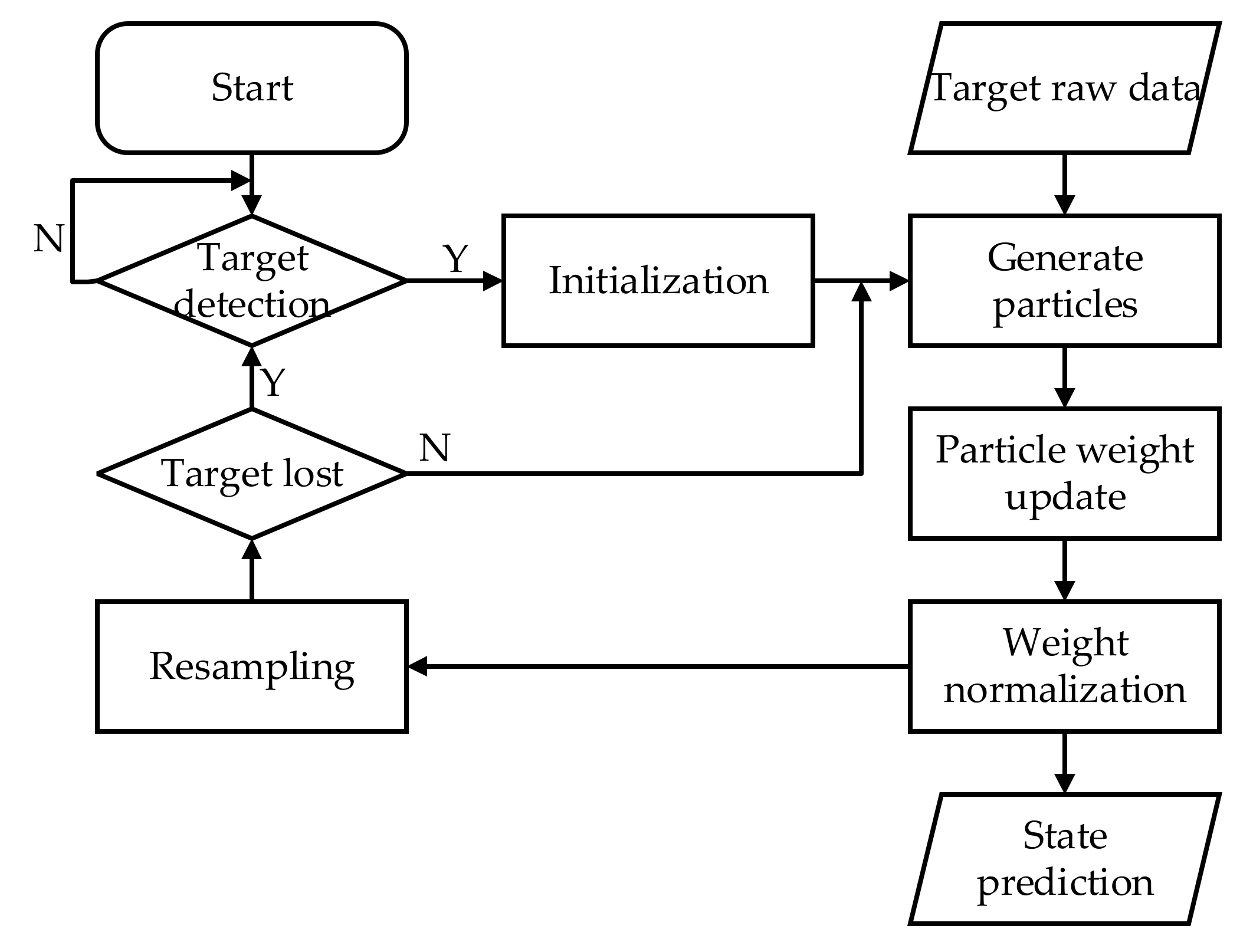
Target Tracking Based on Particle Filter Algorithm

The PF algorithm is a statistical filtering method based on Monte Carlo and recursive Bayesian estimation. Its basic idea is that the posterior probability density of target propagation can be represented by several particles which are very small scale filters. They represent the various possibilities of the target state. In a nonlinear, non-Gaussian system, it has unique advantages in processing parameter estimation and state filtering [30]. It can provide a more accurate position of the target moving object for the grasping task of the robotic arm.

In object detection of the image, there will be problems such as bounce of the bounding box, missed detection, and the wrong detection, so tracking becomes particularly important [31,32]. To simulate a similar catering environment, diversified interferences are supposed to be produced accordingly on the belt. The bowl is just a typical model in the catering industry which can represent an important object in the process of automation development. Moreover, we meet higher requirements for tracking and grasping the bowl as the tiny advance or delay of the gripper could cause the bowl to tilt, making it imperfect to design subsequent automation. Therefore, we use the bowl as the target object for tracking and predicting. In the actual detection environment, the interference of the conveyor belt and the environment has a certain impact on the delivery of the target. Therefore, this paper applies PF related theory to optimize the target tracking and predict the position of the moving target on the conveyor belt. Only by optimizing the target motion curve, predicting its maximum possible position in advance, and moving with the object at the same time to reach the predicted position can the capture be completed.

The target on the conveyor belt generally moves at a constant speed. When the environment produces interference, the conveyor belt speed becomes a non-linear motion. Set the target’s motion state parameter to x_k. In the tracking process, due to the acceleration generated when the target is disturbed, the motion model of the target object will be a 3 × 3 transfer matrix containing position, velocity, and acceleration. The conveyor belt is placed on the XOY plane in the world coordinate system, and the tracking process only requires real-time tracking in the XY direction [9]. If the model contains the motion state information of the x-axis and y-axis, a 6 × 6 transfer matrix will be generated. In practice, the relative position of the conveyor belt and the RGB-D sensor is uncertain, so the linear relationship between the x-axis and y-axis in the trajectory of the target object cannot be accurately obtained. Therefore, it is assumed that x and y are not related to each other in the model. Thus the 6 × 6 transfer matrix in the model is independently formed with two 3 × 3 transfer matrices, where PF is performed on them respectively. The following takes the x-axis direction as an example.

Define the system state by a three-dimensional variable x_k = (xs_k, xv_k, xa_k), which represents the position, velocity, and acceleration of the target in the x-axis. The system states require the following relationships:

$$x{\mathrm{s}}_k=x{\mathrm{s}}_{k-1}+x{v}_{k-1}dt+0.5x{a}_{k-1}d{t}^2$$

(13)

The model of the system is established in Equation (14). dt represents the time interval.

$$\left(\begin{array}{l}x{s}_k\\ x{v}_k\\ x{a}_k\end{array}\right)=\left(\begin{array}{ccc}1& dt& 0.5d{t}^2\\ 0& 1& dt\\ 0& 0& 1\end{array}\right)\left(\begin{array}{l}x{s}_{k-1}\\ x{v}_{k-1}\\ x{a}_{k-1}\end{array}\right)+\left(\begin{array}{c}{q}_1\\ q_2\\ q_3\end{array}\right)$$

(14)

$$x_k=F{x}_{k-1}+Q_k$$

(15)

In Equation (15), x_k represents the optimal state estimation of the system at time k. F represents the state transition matrix of the system. Q_k represents the process noise of the k^th frame, where q₁ is the noise on the position. The q₂ is the noise on the speed, and the q₃ is the noise on the acceleration.

The observation model z_k is established based on the moving target in the image, which is shown in Equation (16).

$$z_k=\left(\begin{array}{ccc}1& 0& 0\end{array}\right)\left(\begin{array}{c}x{s}_k\\ x{v}_k\\ x{a}_k\end{array}\right)+R_k$$

(16)

$$z_k=H{x}_k+R_k$$

(17)

where H is the observation matrix of the system and R_k represents the observation noise at time k.

It is assumed that both the process noise Q_k and the observation noise R obey the Gaussian distribution. The PF is composed of initialization, state update, particle weight update, weight normalization, resampling, state output, and prediction.

(1)

Initialization: with the prior condition probability p(x₀) of the system state, the posterior probability distribution $p(x_{1:k}|z_{1:k}),(x_{1:k}^i,i=1,2,\cdots ,N)$ used to represent the target state ${\{x_{1:k}^i,w_k^i\}}_{k=1}^{N_s}$ at time k represents the sample set of corresponding weights $\{w_k^i,i=1,2,\cdots ,N\}$, where the state set from 0 to k is represented by $x_{1:k}=\{x_j,j=1,2,\cdots ,t\}$.

$$p(x_{1:k}|z_{1:k})\approx {\displaystyle \sum _{i=1}^{N_s}{w}_k^i}\delta (x_{1:k}-x_{1:k}^i)$$

(18)

where $\{w_k^i,i=1,2,\cdots ,N\}$ in Equation (18) is using the expected sampling selection, and Ns is the number of particles sampled to the current moment.

(2)

State update: If the bounding box of object detection appears in successive frames of the system, it means that the object is not subject to false detection. It is necessary to extract the target object according to the detection bounding box and use the importance density function $q(x_{1:k}|z_{1:k})$ to calculate it. The target state particle set ${\left\{x_1^i\right\}}_{i=1}^{N_s}$, particle weight $w_k^i=p(x_{1:k}^i|z_{1:k})/q(x_{1:k}^i|z_{1:k})$, assuming the importance density function, is $q(x_{1:k}|z_{1:k})=q(x_k|z_{1:k-1},z_{1:k})q(x_{1:k-1}|z_{1:k-1})$. From the following Equation (19), a new particle set ${\left\{x_{1:k}^i\right\}}_{i=1}^{N_s}$ can be obtained through the particle set ${\left\{x_1^i\right\}}_{i=1}^{N_s}$ and ${\left\{x_{1:k-1}^i\right\}}_{i=1}^{N_s}$.

$$x_k=F{x}_{k-1}+Q_k$$

(19)

The posterior probability density function is expressed by the following Equation (20).

$$\begin{array}{ll}p(x_{1:k}|z_{1:k})& =\frac{p(z_k|x_{1:k},z_{1:k-1})p(x_{1:k}|z_{1:k-1})}{p(z_k|z_{1:k-1})}\\ & =\frac{p(z_k|x_{1:k},z_{1:k-1})p(x_k|x_{1:k-1},z_{1:k-1})}{p(z_k|z_{1:k-1})}p(x_{1:k-1}|z_{1:k-1})\\ & =\frac{p(z_k|x_k)p(x_k|x_{k-1})}{p(z_k|z_{1:k-1})}p(x_{1:k-1}|z_{1:k-1})\\ & =p(z_k|x_k)p(x_k|x_{k-1})p(x_{1:k-1}|z_{1:k-1})\end{array}$$

(20)

(3)

Particle weight update: When the system predicts and generates the particle set at the next moment according to the transition matrix F, the particle weight is updated according to the following Equation (21).

$$\begin{array}{c}{w}_k^i=\frac{p(z_k|x_k^i)p(x_k^i|x_{k-1}^i)p(x_{1:k-1}^i|z_{1:k-1})}{q(x_k^i|x_{1:k-1}^i,z_{1:k})q(x_{1:k-1}^i|z_{1:k-1})}\\ =w_{k-1}^i\frac{p(z_k|x_k^i)p(x_k^i|x_{k-1}^i)}{q(x_k^i|x_{1:k-1}^i,z_{1:k})}\end{array}$$

(21)

If $q(x_k|x_{1:k-1},z_{1:k})=q(x_k|x_{k-1},z_k)$, then the importance density function only depends on $x_{k-1}$ and $z_k$. It also means that in the calculation process, only the particles ${\left\{x_k^i\right\}}_{i=1}^{N_s}$ need to be stored without considering the particle set ${\left\{x_{1:k-1}^i\right\}}_{i=1}^{N_s}$ and the previous observations $z_{1:k-1}$. The laboratory environment can be regarded as approximate white noise, so $q(x_k^i|x_{1:k-1}^i,z_{1:k})=p(x_k^i|x_{k-1}^i)$. The importance weight value can be expressed as $w_k^i=w_{k-1}^i*p(z_k|x_k^i)$, using the Bhattacharyya distance to calculate the similarity between the reference target template and the candidate template. Based on the similarity measurement, the particle weight update basis is shown as Equation (22):

$$w_k^i=w_{k-1}^i*\frac{1}{{(2\pi R^2)}^{1/2}}{e}^{-\frac{d_i^2}{2R^2}}$$

(22)

$$d_i=x{s}_k-H*{\mathrm{x}}_k$$

(23)

R represents the variance of Gaussian distribution. i represents the ith particle, and $d_i^2$ represents the Bhattacharyya distance of the ith particle.

(4)

Weight normalization: perform the normalization operation of the following equation on the updated particle weights in the model.

$$w_k^i=w_k^i/{\displaystyle \sum _{j=1}^{N_s}{w}_k^j}$$

(24)

(5)

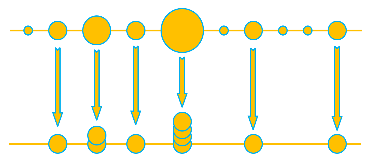
Resampling: since the particles degenerate after multiple iterations, resampling is needed to solve this problem. Particles should be selected based on $w_k^i$. Thus, we could obtain the cumulative distribution function (CDF) as shown in Equation (25).

$$c_k^i=c_k^{i-1}+w_k^i$$

(25)

Then, using binary search algorithm with N particles uniformly distributed in 0–1 random variable to find particles with high weights. Before resampling, the particle sample set and the weight are in an orderly pair ${\{x_k^i,w_k^i\}}_{i=1}^N$. After resampling, they are transformed as ${\{x_k^i,1/N\}}_{i=1}^N$, as shown in Figure 6. The circle in the figure represents the particle and the area represents the weight. Before resampling, the corresponding weight of each particle $x_k^i$ is $w_k^i$. After resampling, the total number of particles remains unchanged. The important particles with heavier weight have multiple particles scattered, while the particles with particularly small weights are discarded. In this way, after resampling, each particle has the same weight, which is 1/N.

(6)

State output: use the weighting criterion as Equation (26) to determine the final position of the target:

$$x_k^{out}={\displaystyle \sum _{i=1}^N{x}_k^i}*w_k^i$$

(26)

(7)

Prediction: In order to use the PF to predict the position of the target object after a certain time Δt of movement, the state information of the target position at the current moment obtained by the RGB-D sensor is output through the PF and then multiplied by the transition matrix F. After repeating Δt/dt times, multiply the observation matrix H to the left to get the next position as Equation (28).

$$x_k^{m+1}=F*x_k^m,\{m=1,2,\cdots ,\frac{\Delta t}{dt}\}$$

(27)

$$x_k^{pre}=H*x_k^{\frac{\Delta t}{dt}}$$

(28)

According to the above initialization, the general process of state update, particle weight update, weight normalization, resampling, state output, and prediction are as shown in Figure 7. The overall target tracking and predicting algorithm based on PF is shown in Algorithm 1.

Algorithm 1. Target object tracking and predicting algorithm based on PF

Target object detection Load current image. Use YOLOv4 to detect the image. Check the target in the image, if not, go to the first step. Initialization Set number of particles as N. Use the center point of the target as the data input (obj_x, obj_y). Set each particle position in x, y direction to obj_x, obj_y. Set the weight of each particle in the x, y direction to 1/N. State update Load current image. Check the target in the image; if not, go to the target object detection step. Calculate the next states of the particles in the x, y direction via (19). Calculate the weight of each particle in the x, y direction via (22) (23). Normalize the weight of each particle via (24). Resampling Generate CDF by weight of particles in the x, y direction. Generate N uniformly distributed variables between 0 and 1 in the x, y direction. For i = 1, 2, …, N Use binary search to find the position of random variables in CDF. The new particle is equal to the old particle in the position. State output Calculate the filtered position of the target via (26). Prediction Calculate the predicted position of the target via (27) (28). Go to the state update step

After such a process of state update-particle weight update-normalization-resampling-output, the PF is used to estimate the position of the target after a certain time Δt, and the trajectory and speed of the robotic arm are planned accordingly. Then the robotic arm can be controlled to complete tracking and grabbing actions.

5. Experiments and Results

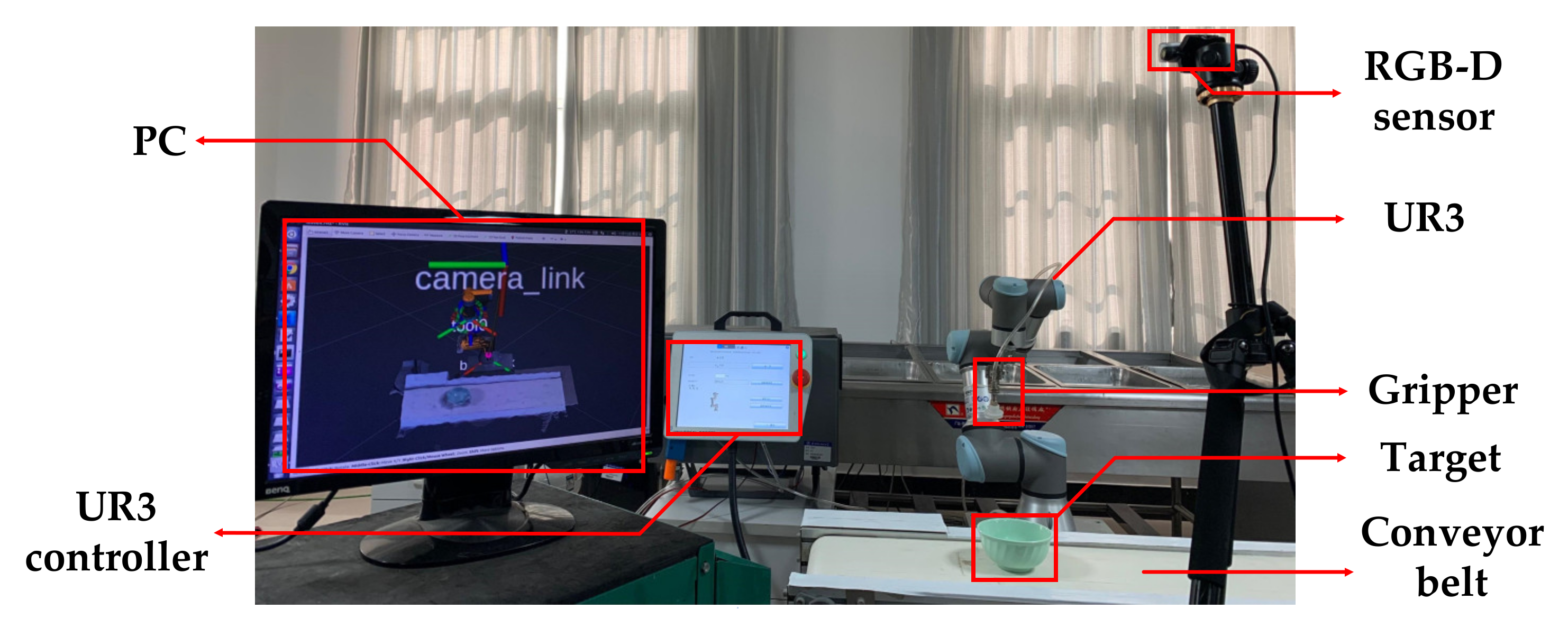
5.1. Experimental Environment and Data Set

The hardware and software environments for the experiments are as follows: a server with Ubuntu 16.04, GTX1080Ti GPU (Nvidia Corporation, Santa Clara, CA, USA) with 11 GB memory, deep learning framework Tensorflow 1.8.0, Keras 2.1.5, Python 3.6, OpenCV 3.4.1.

Before training neural networks or other algorithms, we must first obtain pictures of the target object in each environment as a training set. Taking pictures of the target object in different environments can increase the contrast between the object and the environment to enhance the success rate of recognition. We extracted a total of 6300 pictures for model training and 700 pictures for model testing. Our testing set is available at the site [33]. Our pictures are manually marked with Labellmg, and the rectangular frame information and category information of the target object are stored in an XML file, which is the same format as PASCAL VOC.

5.2. Comparison of Object Detection Algorithms

In order to select the appropriate target detector, we have selected the detectors with better detection effect in recent years for comparison of object detection at different distances. Finally, we selected five objective detectors for comparison, and they all use the same dataset and test set mentioned in Section 5.1. The pre-trained network for Faster R-CNN is res101, batch_size = 8, anchor_scales = [8, 16, 32], anchor_ratios = [0.5, 1, 2], input_size = [600, 1000]. The chosen optimizer is SGD, where leanring_rate = 0.001, momentum = 0.9, decay = 0.0001, gamma = 0.1. The pre-trained network for RetinaNet is resnet50, batch_size = 8, anchor_size = [32, 64, 128, 256, 512], anchor_ratio = [0.5, 1, 2], input_size = [320]. The chosen optimizer is Adam, where learning_rate = 0.00001, clipnorm = 0.001 (for controlling gradient clipping). The pre-trained network of RefineDet is resnet101, batch_size = 8, input_size = [800, 1333]. The chosen optimizer is SGD, where learning_rate = 0.001, momentum = 0.9, decay = 0.0005, gamma = 0.1. The pre-training network for YOLOv3 is yolov3.weight, batch_size = 8, input_size = [416], anchor_size = [(315, 380) (453, 508) (638, 674) (927, 1381) (1309, 1831) (1459, 873) (1703, 1989) (2033, 1336) (2165, 2251)]. The chosen optimizer is Adam, where learning_rate = 0.001, momentum = 0.9, decay = 0.0005.

As shown in

Table 1. Object detector performance comparison.

Methods	APClose	APMedium	APFar	FPS
HSV	90.4%	91.1%	89.5%	-
Faster R-CNN	99.6%	99.7%	99.1%	3
RefineDet [34]	95.1%	96.6%	95.3%	24
RetinaNet [35]	95.5%	95.9%	94.8%	14
YOLOv3	96.1%	97.3%	95.6%	19
YOLOv4	99.3%	99.5%	96.7%	22

Note: AP_close represents the success rate of object detection when the distance between the RGB sensor and the target object is 0.3 m. AP_Medium represents the success rate of object detection when the distance between the RGB sensor and the target object is 0.6 m. AP_Far represents the success rate of object detection when the distance between the RGB sensor and the target object is 1.0 m. The FPS indicates the number of pictures that the model can detect per second.

, although the target in each frame of the image can be identified using the HSV (Hue Saturation Value) method, the interference is also easy to be detected. It has a certain impact on the establishment of the follow-up tracking model. However, a good balance between accuracy and speed can be maintained using YOLOv4. The average recognition accuracy reaches 98.5%, and the FPS remains at about 22 frames. Compared with YOLOv3 or other network algorithms, it improves a lot. Accordingly, it will provide a solid foundation for the follow-up tracking algorithm and reduce the time the target object could lose in the field of vision. Therefore, we chose YOLOv4 as our target object detection algorithm.

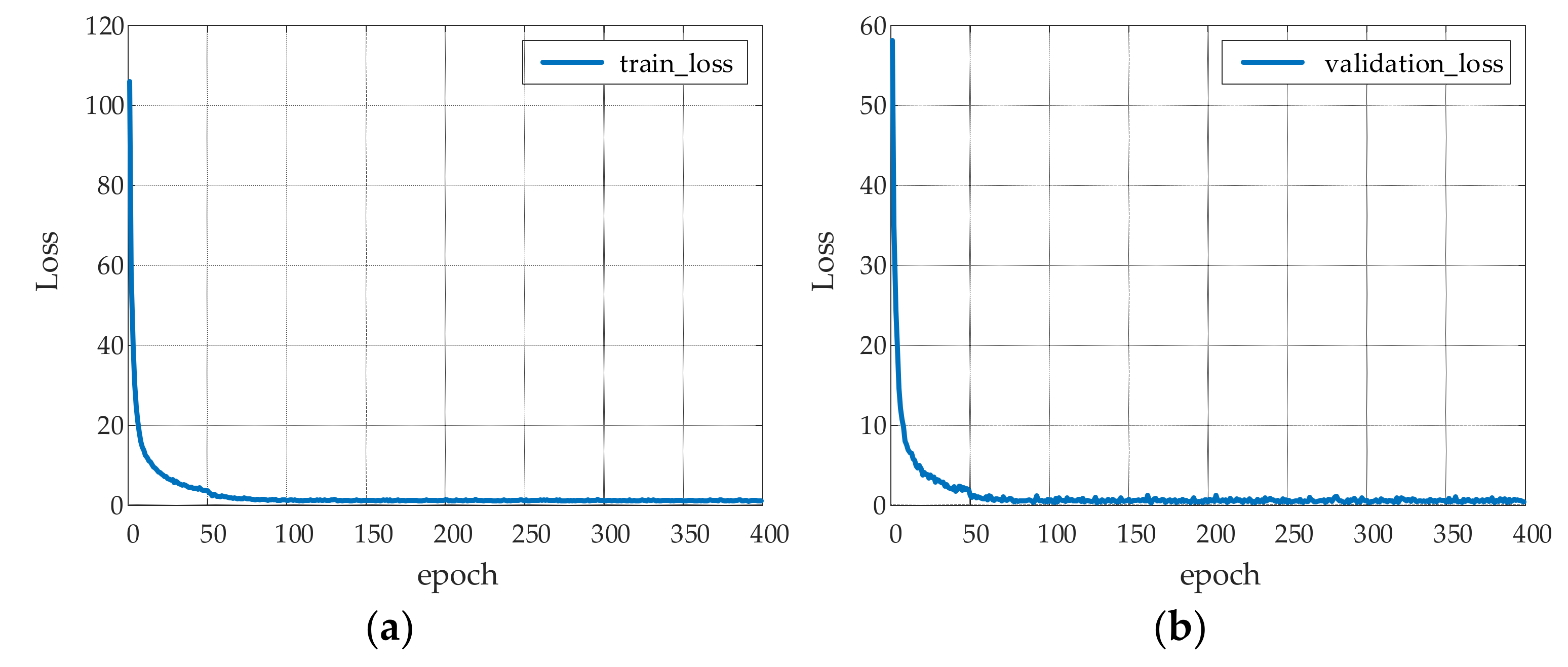
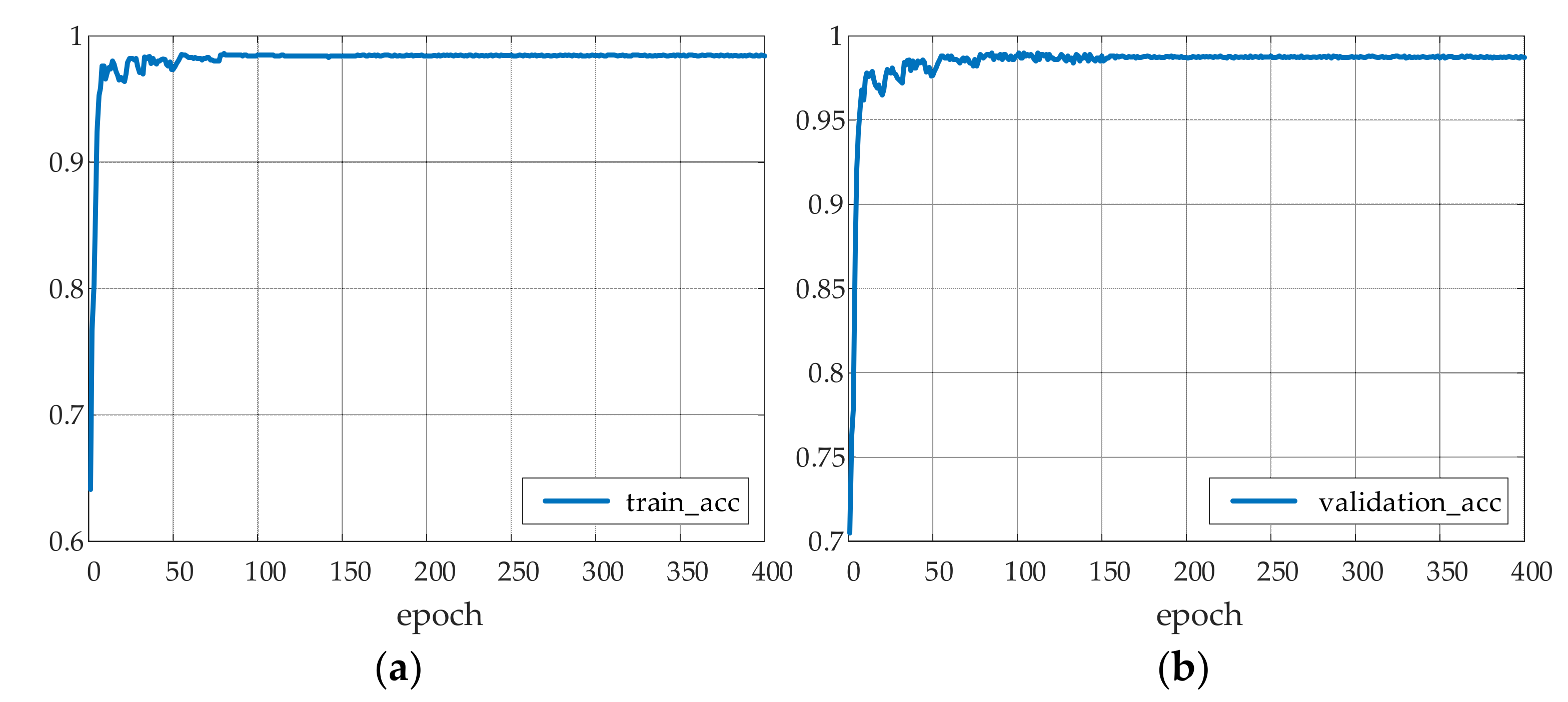
5.3. YOLOv4 Network Training Process and Result Analysis

We used the k-means algorithm to generate anchor points suitable for the dataset by clustering the bounding boxes of the training set to improve the detection of the network. The clustering produced nine sets of anchors and assigned them for use in large, medium, and small scale predictions:

• 76 × 76: (1703, 1989) (2033, 1336) (2165, 2251)
• 38 × 38: (927, 1381) (1309, 1831) (1459, 873)
• 19 × 19: (315, 380) (453, 508) (638,674)

More importantly, the training process of our network is as follows:

We used a single GPU for training. Migration learning was performed using a pre-trained model obtained based on the COCO training set. For the first 50 epochs, the backbone network was first frozen to train the prediction network parameters, and, after obtaining a lower training loss relatively quickly, the backbone network was unfrozen to train the parameters of the whole network. The image input size was 416 × 416, batch_size = 8, and the number of training iterations was initially set to epoch = 400. The training process uses the Adam optimizer for iterative parameter updates. The initial learning rate = 0.001, momentum = 0.9, and decay = 0.1. The current learning rate is decayed to 1/10 when the validation loss is no longer decreasing.

The results of YOLOv4 network training are shown in Figure 8 and Figure 9. A pre-trained model is used in the first 50 epochs of training to freeze the backbone network and perform migration learning to quickly converge to a low loss value. When epoch = 50, the curve has an abnormal fluctuation, and the overall trend of recognition accuracy of the network increases. Then, the backbone network is unfrozen and the parameters of the whole network are trained. The final loss value of the model converges to around 1.1289 and training is terminated. The training model was tested on the test set using the training model, and the test results are shown in Table 1.

The YOLOv4 model after training is used for testing. The resolution of the RGB-D sensor is 640 × 480, and the detection rate is 30 FPS. The detection result is shown below. Figure 10a is the original image of the target object at different positions under the RGB-D sensor; Figure 10b is the feature extraction map of the target object under the YOLOv4 network; and Figure 10c is the bounding box and successful recognition rate detected by the target object.

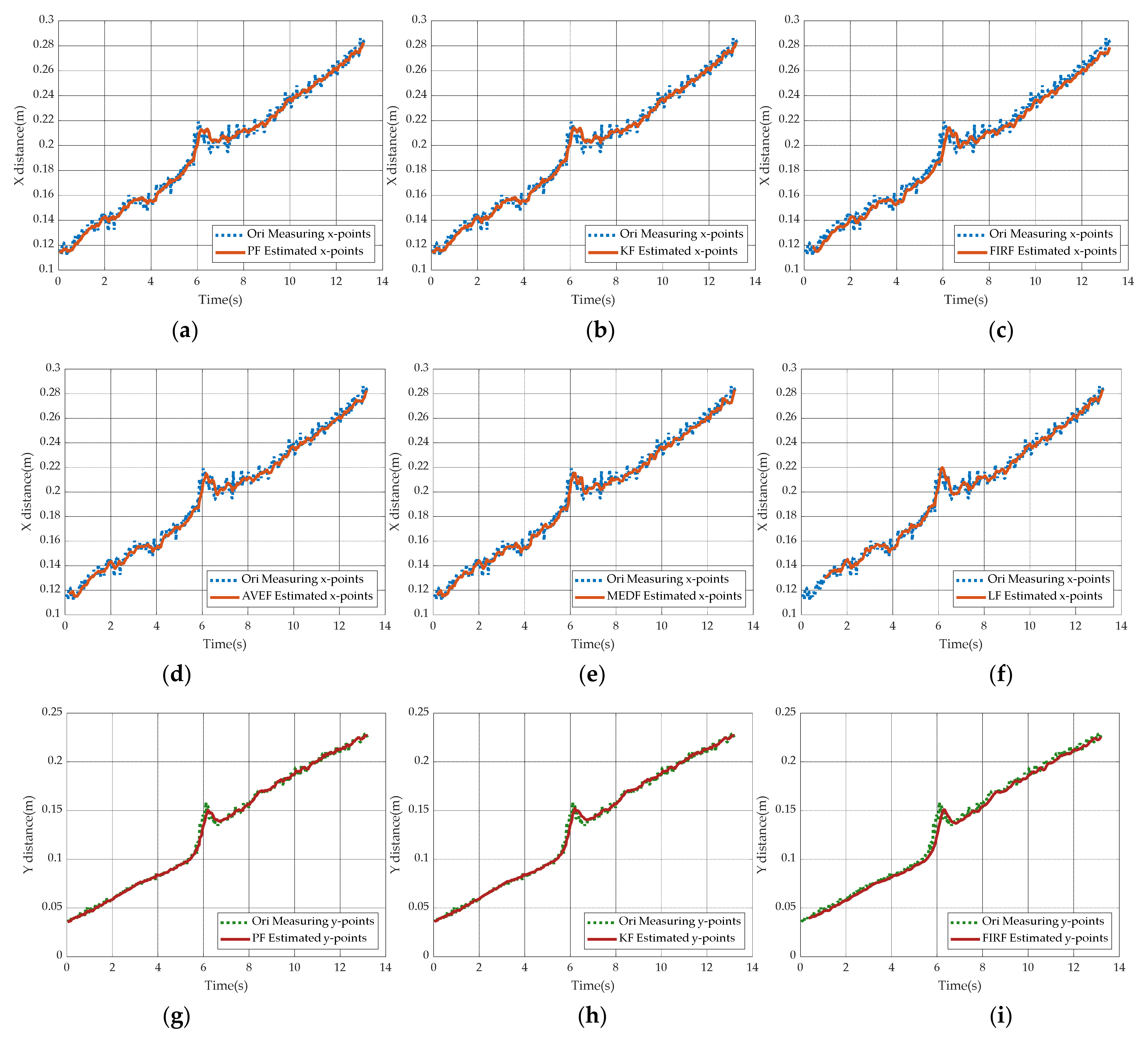
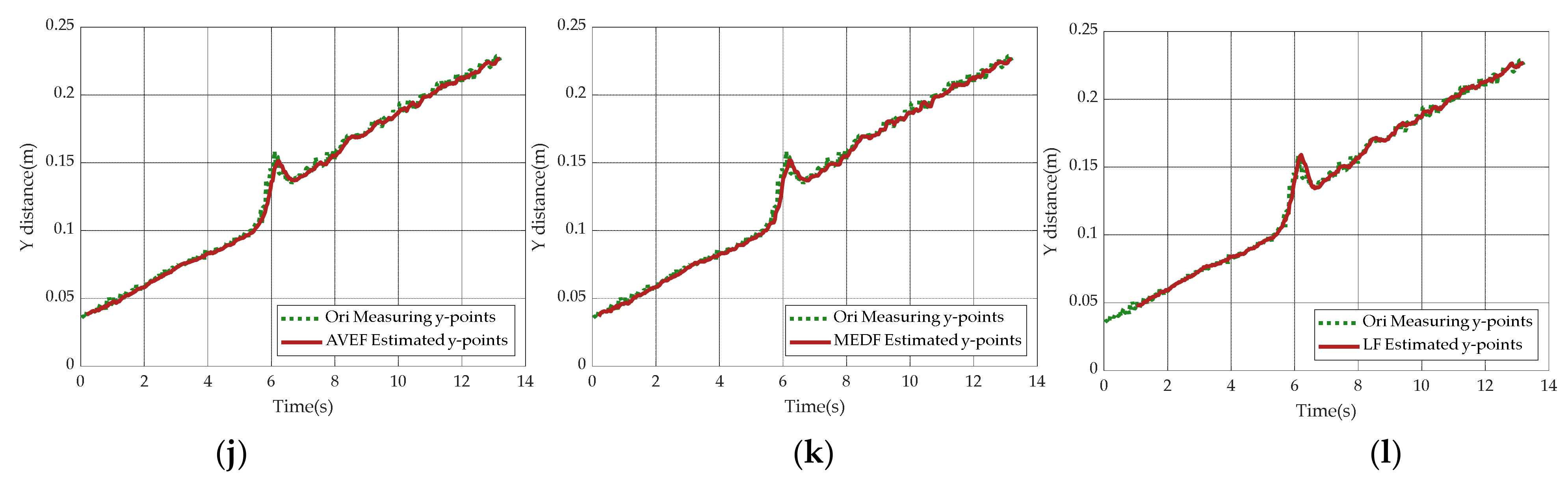
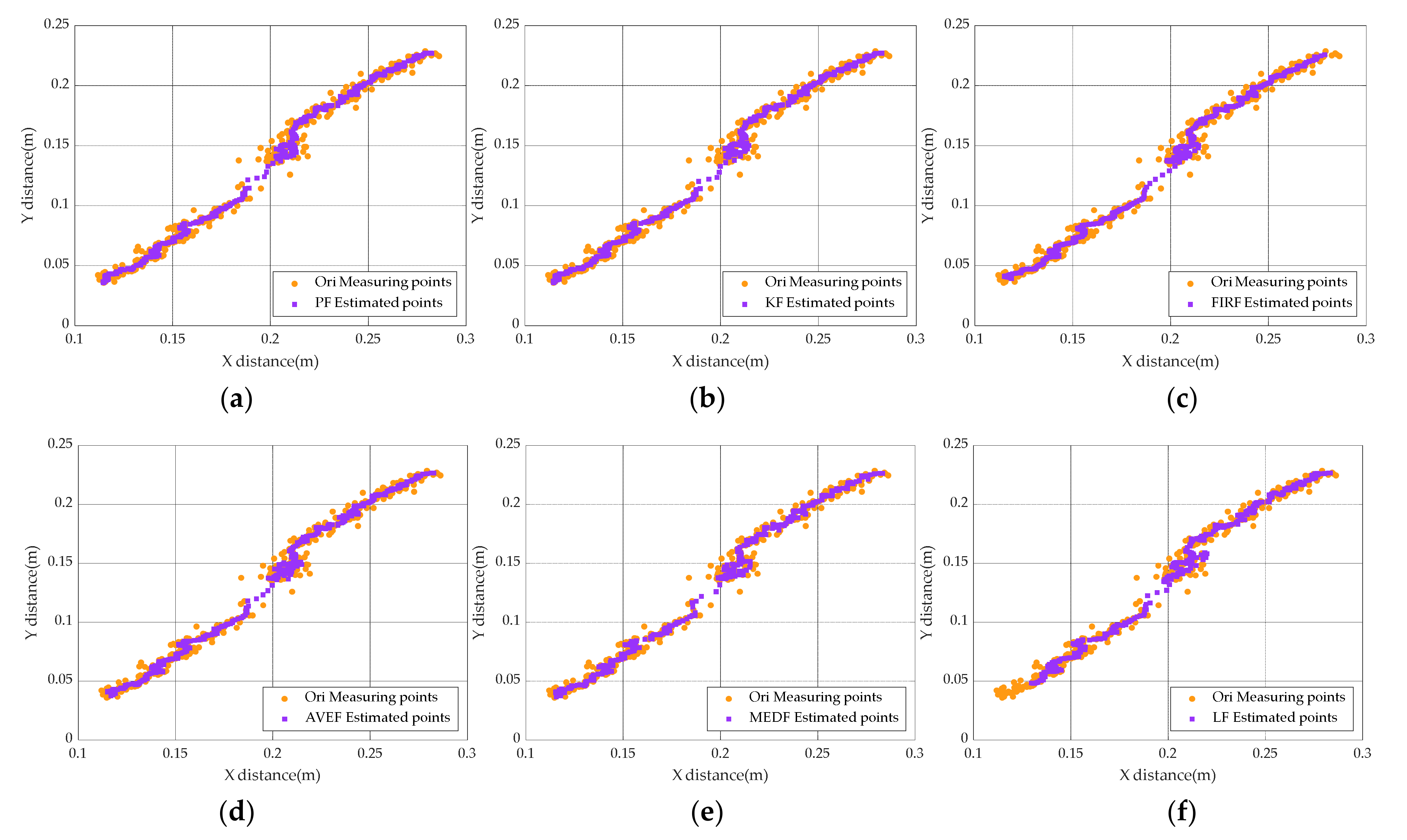
5.4. Simulation Comparison under Different Filter-Based Target Tracking Methods

The real calibration environment has established six filters in Matlab to filter the identified target position curve, namely PF, KF, Finite Impulse Response filter (FIRF), Average filter (AVEF), Median filter (MEDF), and Linear Fit filter (LF). As shown in Figure 11, the original points of the x-axis and y-axis of the target position that change with time are respectively given (Ori Measuring x-points and Ori Measuring y-points), and the filtering effect of the corresponding filter on the corresponding axis is displayed. It can be seen that no matter whether there is environmental interference or not, the FIRF, the AVEF, and the MEDF show a lag in the tracking effect of the target position, which will lead to imprecise tracking of the target object. The reason is that these three filters are the result of the weighted average of current observations and past observations. LF has a positive filtering effect under relatively stable conditions. When there is environmental interference, LF’s regression is slower. LF has no ability to adjust to environmental interference. Compared with them, the tracking performance of PF and KF are stronger, because they have better tracking curves for the target object. PF and KF both belong to the Bayesian filtering system which makes them have the ability to optimize weighting factors in real-time, thus they have certain abilities to adjust. However, if the environment interferes, it is obvious that the regression effect of PF is better than KF. Because KF is based on MSE, it is necessary to make the linear assumption and Gaussian assumptions of posterior probability for the system, whereas PF, a nonlinear and non-Gaussian filter, is based on maximum posterior probability. By comparison, PF has better adaptability.

As shown in Figure 12, this is the motion curve and estimated curve of the target object in the actual two-dimensional plane. It can be seen that the overall curve of the PF is smoother. After non-linear motion occurs in the middle of the image, the estimation points of the six filters are concentrated in the places where X ≈ 0.21 m and Y ≈ 0.14 m. The area where the estimated points of the PF converge is smaller, indicating that the nonlinear motion has the least impact on it. Therefore, we can see the PF’s filtering effect has unique advantages among them.

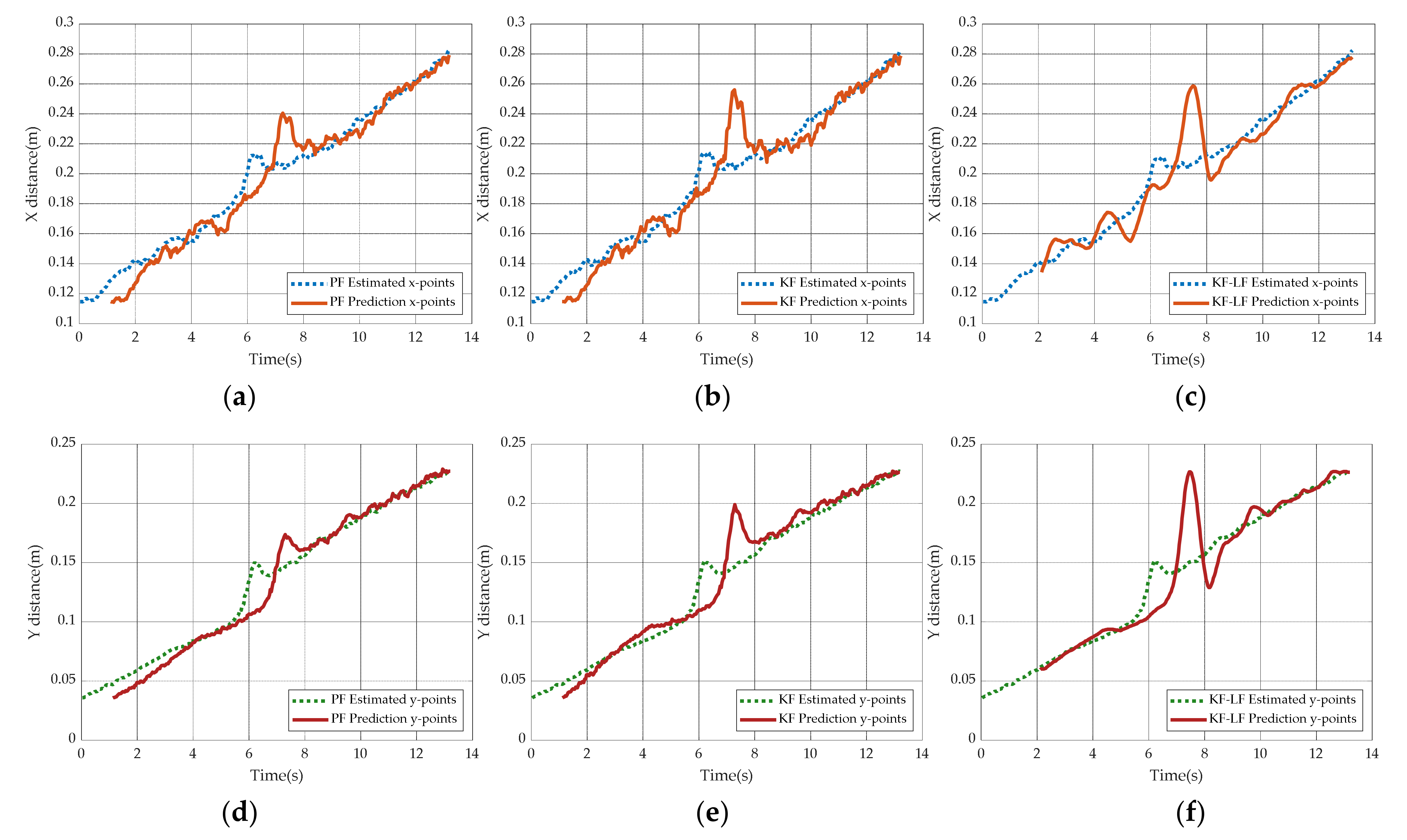
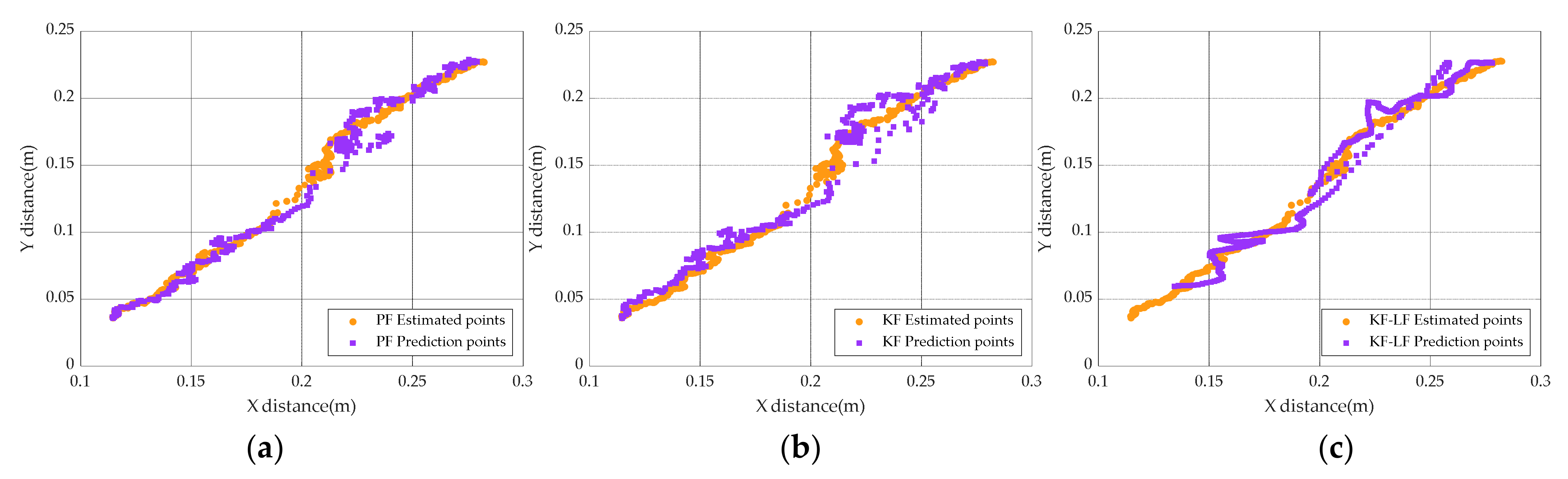
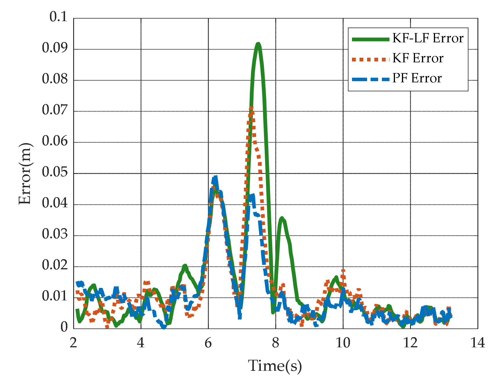
5.5. Simulation Comparison under Different Filter-Based Target Predicting Methods

In order to make the robotic arm reach the grasping point that we want in practice, we must estimate the position of the target at the next moment so that the robotic arm and the target can move to the grasping point at the same time. Therefore, we also need to compare the prediction performance of the filter. From Section 5.3, the six filters can exclude FIRF, AVEF, MEDF, and LF. Considering the estimation performance of linear fitting filter under linear conditions, the filter (KF-LF) combined with KF and LF is added. As shown in Figure 13, it can be seen that in the same environment, KF and KF-LF have a slower strain on environmental interference, and its jitter amplitude is relatively severe. Due to the characteristics of LF, severe oscillations will occur when the predicted step length is lengthened. After the interference is generated, the impact of the interference cannot be eliminated in time, whereas the PF can quickly predict the position of the target at the beginning, and its peak value is relatively small, which can better adapt to environmental changes.

As shown in Figure 14, this is the estimated curve and prediction curve of the two-dimensional plane of the target object. It can be found that PF fits the estimated curve more closely in the overall trend. When the environment is disturbed, its prediction point will not deviate too far. After returning in time, it can continue to steadily fit the estimated curve of the target to make predictions.

As shown in Figure 15, this is the prediction error curve of the three filters. As shown in

Table 2. Mean square error (MSE) of the filters.

Filter	MSE
	Filter Error	Prediction Error
PF	7.1537 × 10−6	1.1356 × 10−4
KF	7.2296 × 10−6	1.8455 × 10−4
FIRF	4.9 × 10−3	-
AVEF	8.1293 × 10−6	-
MEDF	1.0993 × 10−5	-
LF	6.9699 × 10−6	-
KF-LF	-	3.3175 × 10−4

Note: Filter error represents the MSE between the filtered position in the direction of the target object’s movement (including the x direction and y direction) and the original measured position, and the prediction error represents the MSE between the prediction in the direction of the target object’s movement (including the x direction and y direction) and the filtered position in the direction of the target object’s movement (including the x direction and y direction).

, this is the MSE of the filters. It can be seen that the overall error of the PF is smaller which means PF’s ability to cope with environmental interference is stronger. On the whole, the performance of PF in filtering and prediction is relatively good. Therefore, the method of PF prediction will be used to capture the target object in the future. Our testing technical parameter setting is shown in

Table 3. Technical parameter settings.

Parameter	PF	KF	KF-LF
N	32768	-	-
q1	4 × 10−6	5	5
q2	2 × 10−6	2	2
q3	1 × 10−7	0.5	0.5
R	0.0001	100	100
$\Delta t/dt$	30	30	30

Note: N is the number of particles in PF, $dt$ = 0.033 s, $\Delta t$ = 1 s, $\Delta t/dt$ means the times of cycles required to predict the position after 1 s.

.

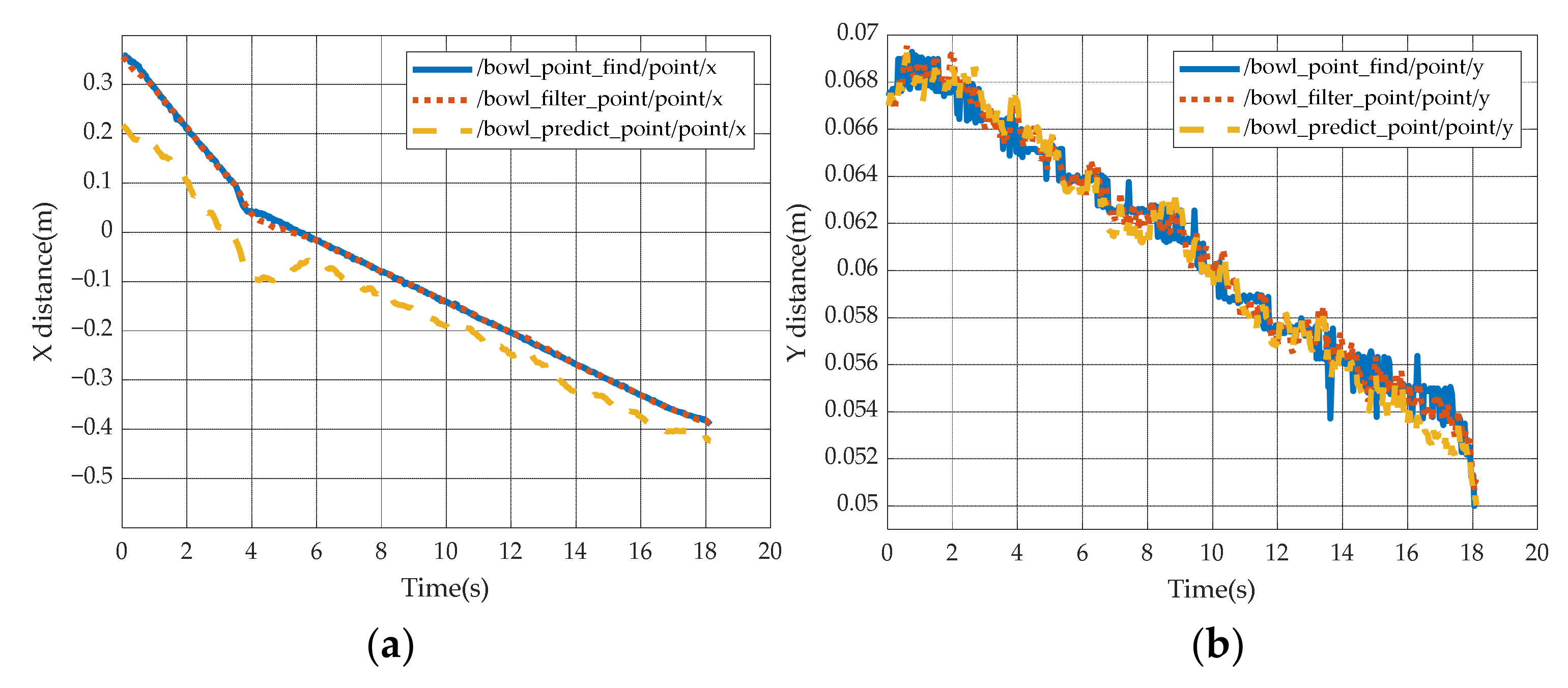
5.6. Particle Filter in Robotic Arm

As shown in Figure 16, this is the position information of the target object measured on the RGB-D sensor. Bowl_point_find is the converted coordinates of the target object in the world coordinate system measured by the RGB-D sensor. Bowl_filter_find is the coordinates of the target object after PF. Bowl_predict_point is the coordinates predicted by PF. Because the changes of the x-axis and y-axis are different, in order to make the picture clearer, this paper separates the information of the x-axis and y-axis into two pictures. From the above figure, it can be clearly seen that the points measured on the sensor are almost linear. After PF, a stable curve can be obtained. When environmental interference occurs, the predicted points will also change quickly to the correct value. Consequently, the successful grabbing that involves the combination of YOLOv4 and PF is going to be studied in the paper.

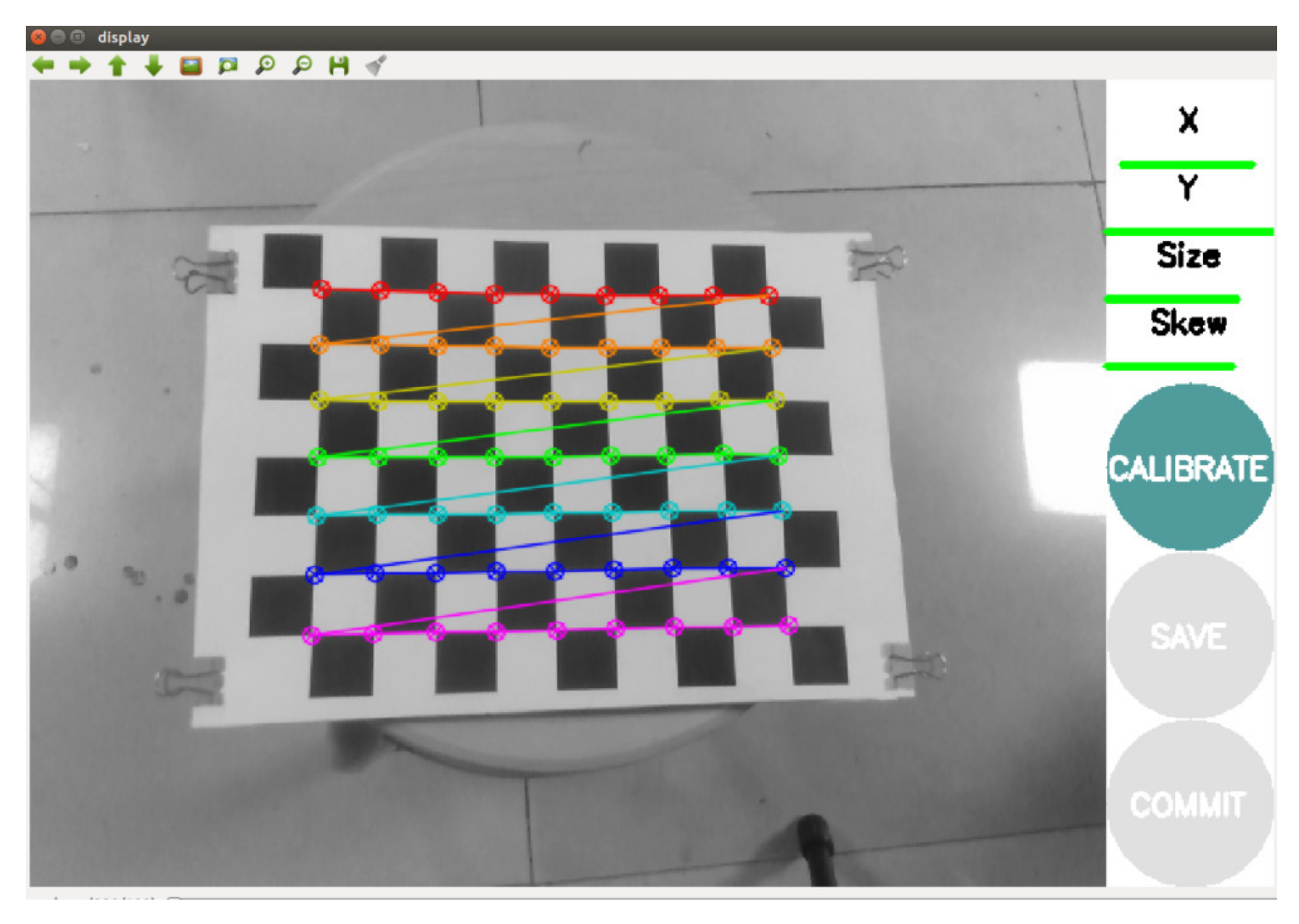
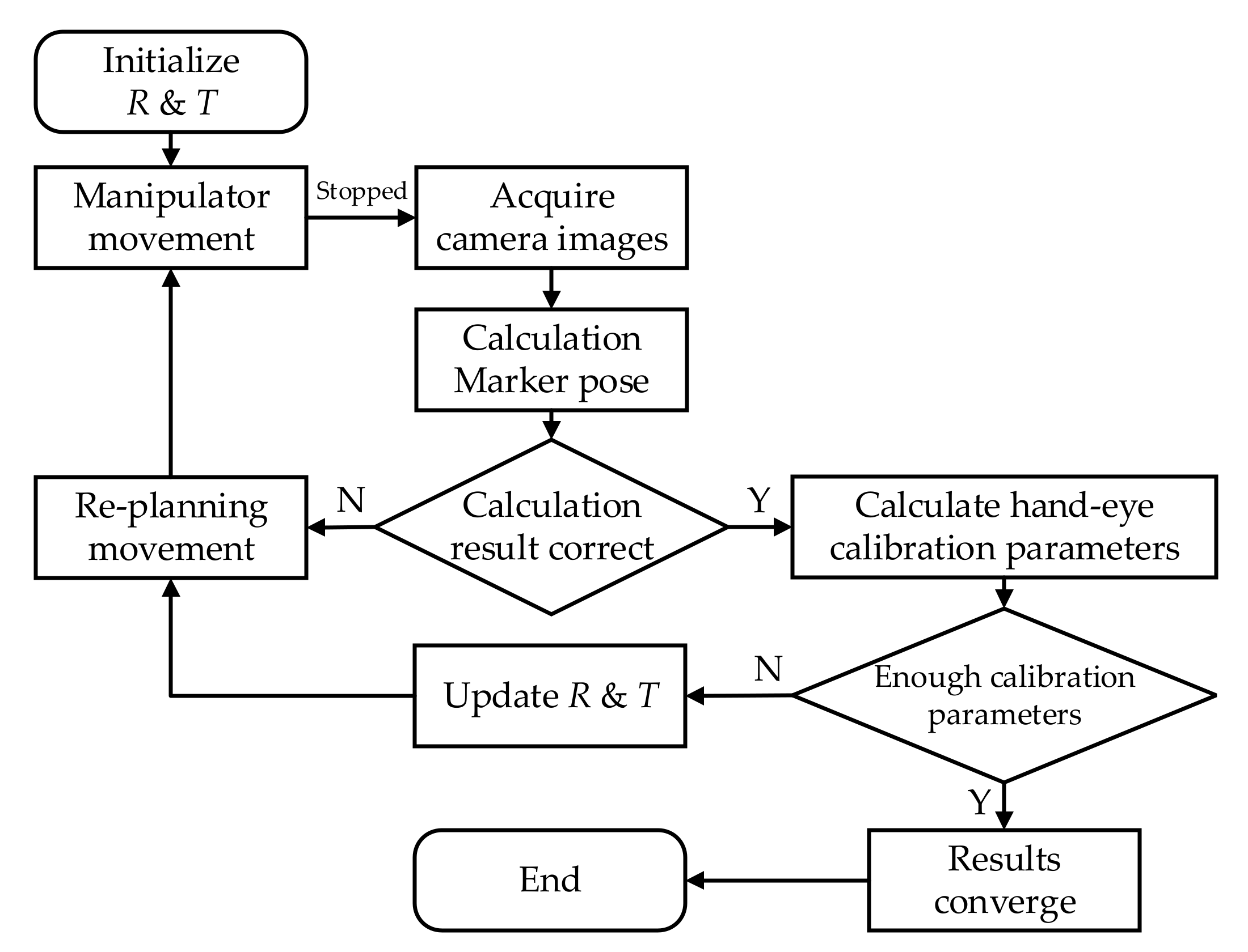
5.7. Eye-to-Hand Calibration System

The software and hardware equipment required to complete the eye-to-hand calibration system are the following: ROS (robot operating system), MoveIt! (motion planning library), VISP (visual servo software) [36,37,38], a PC with Ubuntu 16.04, Realsense D435i camera (Intel Corporation, Santa Clara, CA, USA), marker board, checkerboard calibration board, and a UR3 robotic arm (Universal Robot Corporation, Odense, Denmark).

The whole calibration process of the camera is divided into two parts. They are the internal calibration parameters and the external calibration parameters. The internal calibration parameters remove the effect of camera distortion, and the external calibration parameters calibrate the depth measurement of the camera. The internal parameters calibration uses the Zhang Zhengyou calibration method [39], which uses a 9 × 7 checkerboard calibration board with a grid size of 24.5 mm to calculate the internal parameters and distortion parameters of the camera through its calculation at each angle in the camera’s field of view as shown in Figure 17.

The camera external parameters calibration is done by eye-to-hand calibration. Where the depth sensor of the camera is used to calibrate the position of the marker board at the end of the robot arm from the camera. Through the eye-to-hand calibration procedure, as shown in Figure 18, by calculating the different positions of the Marker boards relative to the end of the robotic arm, the coordinate transformation matrix of the camera relative to the robotic arm coordinate system can be finally obtained. The coordinate transformation matrix consists of a rotation matrix R and a translation matrix T. The specific values are shown in

Table 4. Calibration parameters.

Internal parameters	fx (Normalized focal length on the x-axis):	617.0269
	fy (Normalized focal length on the y-axis):	616.1555
	m0 (Image center horizontal coordinate):	325.1717
	n0(Image center vertical coordinate):	225.4922
Distortion	0.1601, −0.3411, −0.0057, −0.0013, 0
T	position x:	0.4242
	position y:	0.5054
	position z:	0.8581
R	orientation x:	0.5391
	orientation y:	0.2321
	orientation z:	−0.7407
	orientation w:	0.3267

.

Then we can obtain the conversion relation of the target point in the pixel coordinate system to the world coordinate system according to Equation (29).

$$Z_c\left[\begin{array}{c}m\\ n\\ 1\end{array}\right]=\left[\begin{array}{cccc}{f}_x& 0& m_0& 0\\ 0& f_y& n_0& 0\\ 0& 0& 1& 0\end{array}\right]\left[\begin{array}{cc}R& T\\ \overrightarrow{0}& 1\end{array}\right]\left[\begin{array}{c}{X}_W\\ Y_W\\ Z_W\\ 1\end{array}\right]$$

(29)

where m, n are the coordinates of the target point under the pixel coordinate system and X_w, Y_w, Z_w are the coordinates of the target point under the world coordinate system. Then, we load the above parameters through ROS and publish them to TF (TransForm) to get the calibrated target points.

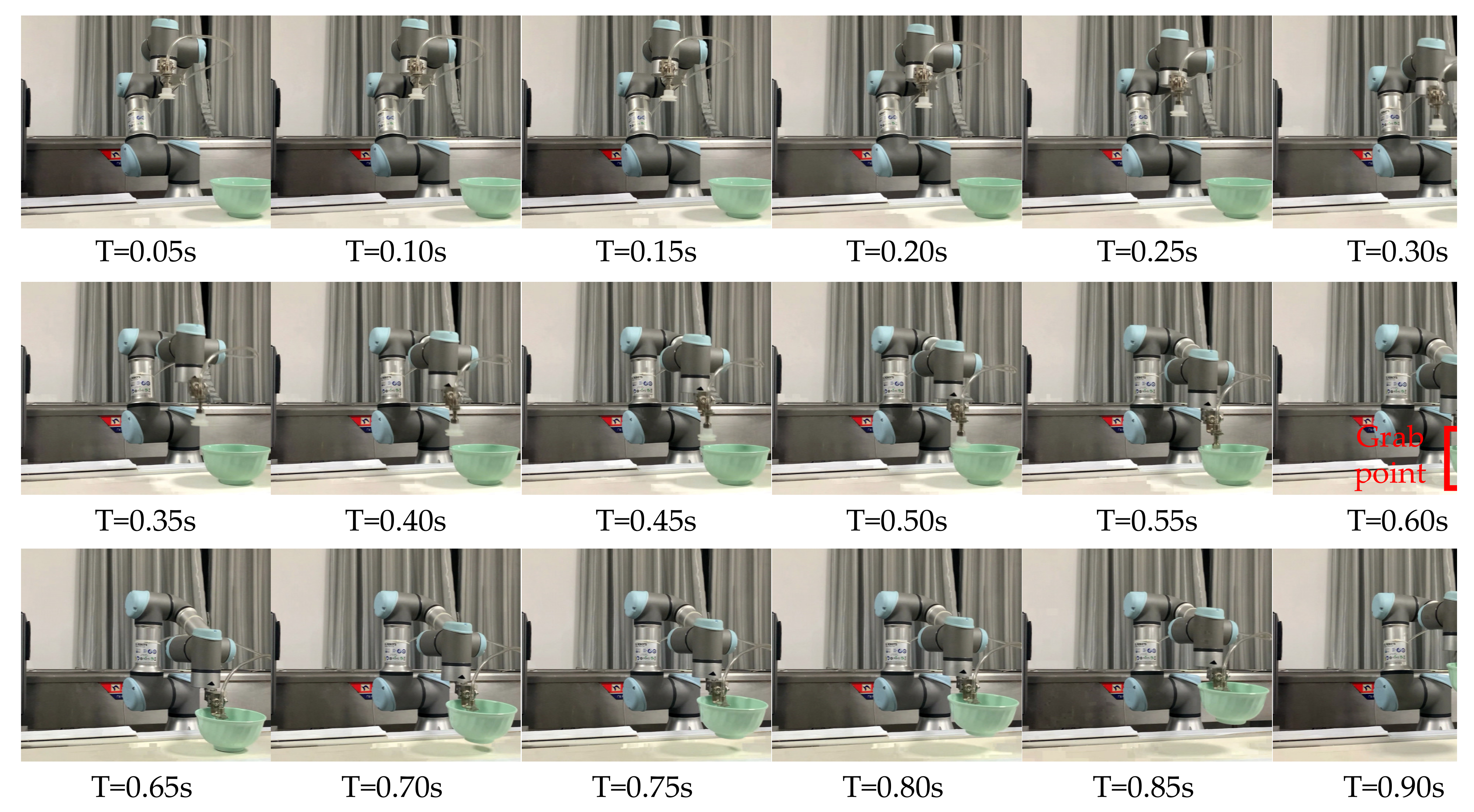
5.8. Experiment of Robotic Arm Tracking, Predicting and Grabbing

In order to verify this robotic arm grabbing system, the experimental environment is set up as shown in Figure 19:

The tracking and predicting grabbing system of the robotic arm is roughly divided into the following four parts:

• Firstly, get the predicted points captured by the robotic arm according to the PF as shown in Figure 20.
• Secondly, plan the path of the robotic arm to the predicted point through MoveIt!.
• Thirdly, the UR3 controller powers on the gripper. Powering on in advance will reduce the waiting time of the gripper at the grab point so that the grab action can be completed more efficiently.
• Finally, the UR3 controller controls the robotic arm to reach the designed grab point according to the planned path. After completing the grab, it will then leave. And the experimental results are shown in Figure 21.

To further illustrate the performance benefits of the proposed robotic arm grabbing system, comparative simulations were performed in this paper. We put the target object on the conveyor belt to make it have different initial speeds, and give it a nonlinear disturbance when it moves to the middle process. Then we repeated the experiment 500 times to compare their performance. The specific results are shown in

Table 5. Performance comparative results.

Aq	v = 2 cm/s	v = 6 cm/s	v = 10 cm/s	v = 14 cm/s
PF	98.20%	95.40%	91.60%	88.60%
KF	92.40%	90.60%	86.60%	84.00%

Note: Aq is the average quality of grabbing.

:

6. Conclusions

The robotic arm grabbing system based on YOLOv4 and PF in the nonlinear and non-Gaussian environment is deeply studied in this paper. Specifically, the moving targets can be identified with the utilization of the YOLOv4 algorithm and the target position can be tracked and predicted with the utilization of the PF algorithm. On this basis, the detection experiment of the YOLOv4 algorithm and a large number of simulation comparison experiments between the filters have been carried out, which reflects the high accuracy and real-time performance of the YOLOv4 algorithm, as well as the ability to adjust rapidly of the PF under interference. Then the robotic arm can cooperate with the path planning function of MoveIt! to realize the rapid grasp of the target object. The results show that the implementation of this system is highly effective. Consequently, it is extremely conducive to improve intelligence in the robot industry.

In this paper, we design a robotic arm grabbing system that can be applied to grasp objects with nonlinear motion. The method not only ensures the accuracy of recognition of target objects, but also satisfies the ability to predict the motion trend of target objects. In the future development of new disciplines such as artificial intelligence, image processing, and the need for tracking and grasping of flexible robots and dual-arm robots, having a reliable and stable grabbing system will play a very important role. In the future, we will try to apply this system to flexible robots or dual-arm robots, and cooperate with their respective characteristics to further improve the robotic arm system so as to accomplish specific operational tasks.

References

1. Strandhagen, J.W.; Alfnes, E.; Strandhagen, J.O.; Vallandingham, L.R. The fit of Industry 4.0 applications in manufacturing logistics: A multiple case study. Adv. Manuf. 2017, 5, 344–358. [Google Scholar] [CrossRef] [Green Version]
2. Su, S.; Xu, Z.; Yang, Y. Research on Robot Vision Servo Based on image big data. J. Phys. Conf. Ser. 2020, 1650, 032132. [Google Scholar] [CrossRef]
3. Lu, C. Kalman tracking algorithm of ping-pong robot based on fuzzy real-time image. J. Intell. Fuzzy Syst. 2020, 38, 1–10. [Google Scholar] [CrossRef]
4. Zhang, Y.; Cheng, W. Vision-based robot sorting system. In IOP Conference Series: Materials Science and Engineering, Proceedings of the International Conference on Manufacturing Technology, Materials and Chemical Engineering, Wuhan, China, 14–16 June 2019; IOP Publishing: Bristol, UK, 2019; Volume 592, p. 012154. [Google Scholar]
5. Ren, Y.; Sun, H.; Tang, Y.; Wang, S. Vision Based Object Grasping of Robotic Manipulator. In Proceedings of the 2018 24th International Conference on Automation and Computing, Newcastle upon Tyne, UK, 6–7 September 2018; pp. 1–5. [Google Scholar]
6. Marturi, N.; Kopicki, M.; Rastegarpanah, A.; Rajasekaran, V.; Adjigble, M.; Stolkin, R.; Leonardis, A.; Bekiroglu, Y. Dynamic grasp and trajectory planning for moving objects. Auton. Robot. 2019, 43, 1241–1256. [Google Scholar] [CrossRef]
7. Zhou, H.; Chou, W.; Tuo, W.; Rong, Y.; Xu, S. Mobile Manipulation Integrating Enhanced AMCL High-Precision Location and Dynamic Tracking Grasp. Sensors 2020, 20, 6697. [Google Scholar] [CrossRef]
8. Redmon, J.; Divvala, S.; Girshick, R.; Farhadi, A. You only look once: Unified, real-time object detection. In Proceedings of the IEEE Conference on Computer Vision and Pattern Recognition, Las Vegas, NV, USA, 27–30 June 2016; pp. 779–788. [Google Scholar]
9. Zhao, Y.; Li, H. Positioning and Grabbing Technology of Industrial Robot Based on Vision. Acad. J. Manuf. Eng. 2019, 17, 137–145. [Google Scholar]
10. Wei, H.; Peng, D.; Zhu, X.; Wu, D. A target tracking algorithm for vision based sea cucumber grabbing. In Proceedings of the 2016 IEEE International Conference on Information and Automation, Ningbo, China, 1–3 August 2016; pp. 608–611. [Google Scholar]
11. Kang, H.; Zhou, H.; Wang, X.; Chen, C. Real-time fruit recognition and grasping estimation for robotic apple harvesting. Sensors 2020, 20, 5670. [Google Scholar] [CrossRef]
12. Redmon, J.; Farhadi, A. Yolov3: An incremental improvement. arXiv 2018, arXiv:1804.02767. Available online: https://arxiv.org/abs/1804.02767 (accessed on 8 December 2020).
13. Liu, W.; Anguelov, D.; Erhan, D.; Szegedy, C.; Reed, S.; Fu, C.Y.; Berg, A.C. Ssd: Single shot multibox detector. In Proceedings of the European Conference on Computer Vision, Amsterdam, The Netherlands, 11–14 October 2016; pp. 21–37. [Google Scholar]
14. He, K.; Gkioxari, G.; Dollár, P.; Girshick, R. Mask r-cnn. In Proceedings of the IEEE International Conference on Computer Vision, Venice, Italy, 22–29 October 2017; pp. 2961–2969. [Google Scholar]
15. Cai, Z.; Vasconcelos, N. Cascade r-cnn: Delving into high quality object detection. In Proceedings of the IEEE Conference on Computer Vision and Pattern Recognition, Salt Lake City, UT, USA, 18–22 June 2018; pp. 6154–6162. [Google Scholar]
16. Rajendran, S.P.; Shine, L.; Pradeep, R.; Vijayaraghavan, S. Real-time traffic sign recognition using YOLOv3 based detector. In Proceedings of the 2019 10th International Conference on Computing, Communication and Networking Technologies, Kanpur, India, 6–8 July 2019; pp. 1–7. [Google Scholar]
17. Peng, J.; Liu, W.; You, T.; Wu, B. Improved YOLO-V3 Workpiece Detection Method for Sorting. In Proceedings of the 2020 5th International Conference on Robotics and Automation Engineering, Guangzhou, China, 19–22 November 2020; pp. 70–75. [Google Scholar]
18. Bochkovskiy, A.; Wang, C.Y.; Liao, H.Y.M. YOLOv4: Optimal Speed and Accuracy of Object Detection. arXiv 2020, arXiv:2004.10934. Available online: https://arxiv.org/abs/2004.10934 (accessed on 8 December 2020).
19. Hong, Z.; Xu, L.; Chen, J. Artificial evolution based cost-reference particle filter for nonlinear state and parameter estimation in process systems with unknown noise statistics and model parameters. J. Taiwan Inst. Chem. Eng. 2020, 112, 377–387. [Google Scholar] [CrossRef]
20. Patel, H.A.; Thakore, D.G. Moving object tracking using kalman filter. Int. J. Comput. Sci. Mob. Comput. 2013, 2, 326–332. [Google Scholar]
21. Weng, S.K.; Kuo, C.M.; Tu, S.K. Video object tracking using adaptive Kalman filter. J. Vis. Commun. Image Represent. 2006, 17, 1190–1208. [Google Scholar] [CrossRef]
22. Arulampalam, M.S.; Maskell, S.; Gordon, N.; Clapp, T. A tutorial on particle filters for online nonlinear/non-Gaussian Bayesian tracking. IEEE Trans. Signal Process. 2002, 50, 174–188. [Google Scholar] [CrossRef] [Green Version]
23. Yang, J.; Schonfeld, D.; Mohamed, M. Robust video stabilization based on particle filter tracking of projected camera motion. IEEE Trans. Circuits Syst. Video Technol. 2009, 19, 945–954. [Google Scholar] [CrossRef]
24. Bastani, V.; Marcenaro, L.; Regazzoni, C. A particle filter based sequential trajectory classifier for behavior analysis in video surveillance. In Proceedings of the 2015 IEEE International Conference on Image Processing, Quebec City, QC, Canada, 27–30 September 2015; pp. 3690–3694. [Google Scholar]
25. Jiang, Z.; Zhao, L.; Li, S.; Jia, Y. Real-time object detection method based on improved YOLOv4-tiny. arXiv 2020, arXiv:2011.04244. Available online: https://arxiv.org/abs/2011.04244 (accessed on 8 December 2020).
26. Ju, M.; Luo, H.; Wang, Z.; Hui, B.; Chang, Z. The application of improved YOLO V3 in multi-scale target detection. Appl. Sci. 2019, 9, 3775. [Google Scholar] [CrossRef] [Green Version]
27. Zhu, Q.; Zheng, H.; Wang, Y.; Cao, Y.; Guo, S. Study on the Evaluation Method of Sound Phase Cloud Maps Based on an Improved YOLOv4 Algorithm. Sensors 2020, 20, 4314. [Google Scholar] [CrossRef]
28. Huang, Y.Q.; Zheng, J.C.; Sun, S.D.; Yang, C.F.; Liu, J. Optimized YOLOv3 Algorithm and Its Application in Traffic Flow Detections. Appl. Sci. 2020, 10, 3079. [Google Scholar] [CrossRef]
29. Kim, W.; Cho, H.; Kim, J.; Kim, B.; Lee, S. YOLO-Based Simultaneous Target Detection and Classification in Automotive FMCW Radar Systems. Sensors 2020, 20, 2897. [Google Scholar] [CrossRef]
30. Chang, C.; Ansari, R. Kernel particle filter for visual tracking. IEEE Signal Process. Lett. 2005, 12, 242–245. [Google Scholar] [CrossRef]
31. Smeulders, A.W.; Chu, D.M.; Cucchiara, R.; Calderara, S.; Dehghan, A.; Shah, M. Visual tracking: An experimental survey. Ieee Trans. Pattern Anal. Mach. Intell. 2013, 36, 1442–1468. [Google Scholar]
32. Gong, Z.; Qiu, C.; Tao, B.; Bai, H.; Yin, Z.; Ding, H. Tracking and grasping of moving target based on accelerated geometric particle filter on colored image. Sci. China Technol. Sci. 2020, 64, 755–766. [Google Scholar] [CrossRef]
33. Bowl Test Set. Available online: https://github.com/Caiyu51/Bowl_test_set (accessed on 7 December 2020).
34. Lin, T.Y.; Goyal, P.; Girshick, R.; He, K.; Dollár, P. Focal loss for dense object detection. In Proceedings of the IEEE International Conference on Computer Vision, Venice, Italy, 22–29 October 2017; pp. 2980–2988. [Google Scholar]
35. Zhang, S.; Wen, L.; Bian, X.; Lei, Z.; Li, S.Z. Single-shot refinement neural network for object detection. In Proceedings of the IEEE Conference on Computer Vision and Pattern Recognition, Salt Lake City, UT, USA, 18–22 June 2018; pp. 4203–4212. [Google Scholar]
36. Quigley, M.; Conley, K.; Gerkey, B.; Faust, J.; Foote, T.; Leibs, J.; Berger, E.; Wheeler, R.; Ng, A. ROS: An open-source Robot Operating System. In Proceedings of the ICRA Workshop on Open Source Software, Kobe, Japan, 17 May 2009; Volume 3, p. 5. [Google Scholar]
37. Chitta, S. MoveIt!: An introduction. In Robot Operating System (ROS); Springer: Cham, Switzerland, 2016; pp. 3–27. [Google Scholar]
38. Marchand, É.; Spindler, F.; Chaumette, F. ViSP for visual servoing: A generic software platform with a wide class of robot control skills. IEEE Robot. Autom. Mag. 2005, 12, 40–52. [Google Scholar] [CrossRef] [Green Version]
39. Zhang, Z. A flexible new technique for camera calibration. IEEE Trans. Pattern Anal. Mach. Intell. 2000, 22, 1330–1334. [Google Scholar] [CrossRef] [Green Version]
Figure 1. Overall flow chart.
Electronics 10 01140 g001
Figure 2. Structure of YOLOv4 algorithm.
Electronics 10 01140 g002
Figure 3. Euclidean distance schematic diagram.
Electronics 10 01140 g003
Figure 4. Target object’s position in the image.
Electronics 10 01140 g004
Figure 5. Difference between YOLOv3 and YOLOv4.
Electronics 10 01140 g005
Figure 6. Resampling schematic diagram.
Electronics 10 01140 g006
Figure 7. Particle filter (PF) process.
Electronics 10 01140 g007
Figure 8. Loss function curves: (a) is the training loss of YOLOv4; (b) is the validation loss of YOLOv4.
Electronics 10 01140 g008
Figure 9. Accuracy test curves: (a) is the training accuracy of YOLOv4; (b) is the validation accuracy of YOLOv4.
Electronics 10 01140 g009
Figure 10. YOLOv4 detect result: (a) Input images; (b) Feature extraction maps; (c) Output images.
Electronics 10 01140 g010
Figure 11. Comparison of the filter effect of different filters under nonlinear conditions on the x-axis and y-axis: (a) is the effect of PF on the x-axis direction; (b) is the effect of Kalman filter (KF) on the x-axis direction; (c) is the effect of finite impulse response filter (FIRF) on the x-axis direction; (d) is the effect of average filter (AVEF) on the x-axis direction; (e) is the effect of median filter (MEDF) on the x-axis direction; (f) is the effect of linear fit filter (LF) on the x-axis direction; (g) is the effect of PF on the y-axis direction; (h) is the effect of KF on the y-axis direction; (i) is the effect of FIRF on the y-axis direction; (j) is the effect of AVEF on the y-axis direction; (k) is the effect of MEDF on the y-axis direction; (l) is the effect of LF on the y-axis direction.
Electronics 10 01140 g011aElectronics 10 01140 g011b
Figure 12. Comparison of the filter effect of different filters under nonlinear conditions in the two-dimensional plane: (a) is the effect of PF in the two-dimensional plane; (b) is the effect of KF in the two-dimensional plane; (c) is the effect of FIRF in the two-dimensional plane; (d) is the effect of AVEF in the two-dimensional plane; (e) is the effect of MEDF in the two-dimensional plane; (f) is the effect of LF in the two-dimensional plane.
Electronics 10 01140 g012
Figure 13. Comparison of the prediction effect of different filters under nonlinear conditions on the x-axis and y-axis: (a) is the effect of PF on the x-axis; (b) is the effect of KF on the x-axis; (c) is the effect of KF-LF on the x-axis; (d) is the effect of PF on the y-axis; (e) is the effect of KF on the y-axis; (f) is the effect of KF-LF on the y-axis.
Electronics 10 01140 g013
Figure 14. Comparison of the prediction effect of different filters under nonlinear conditions in the two-dimensional plane: (a) is the effect of PF in the two-dimensional plane; (b) is the effect of KF in the two-dimensional plane; (c) is the effect of KF-LF in the two-dimensional plane.
Electronics 10 01140 g014
Figure 15. Prediction error curve of the three filters.
Electronics 10 01140 g015
Figure 16. The prediction effect of PF in actual by rqt_plot: (a) is the effect of PF on the x-axis; (b) is the effect of PF on the y-axis.
Electronics 10 01140 g016
Figure 17. Camera internal parameters calibration.
Electronics 10 01140 g017
Figure 18. Eye-to-hand calibration process.
Electronics 10 01140 g018
Figure 19. Grabbing experimental scenes.
Electronics 10 01140 g019
Figure 20. Predicting in PF.
Electronics 10 01140 g020
Figure 21. Tracking and grabbing experiment.
Electronics 10 01140 g021