
Nonlinear Model Predictive Control of Single-Link Flexible-Joint Robot Using Recurrent Neural Network and Differential Evolution Optimization


Abstract
:
1. Introduction
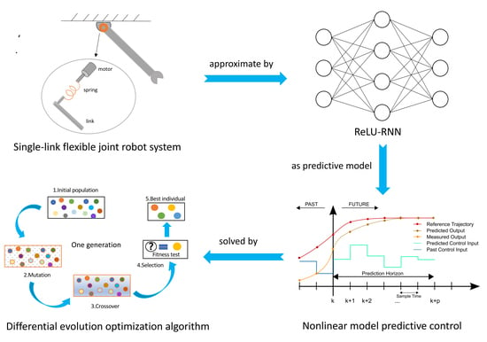
- First, an RNN and DEO based NMPC method is proposed for the position control of a single-link FJ robot. The merit of this process is that not only is the control precision satisfied, but also the overshoots and the residual vibration is well suppressed.
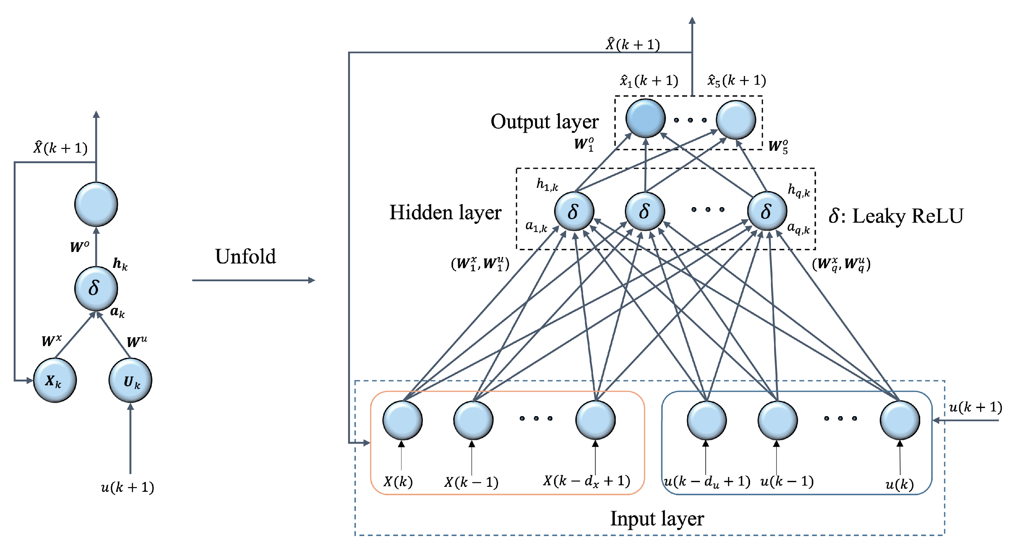
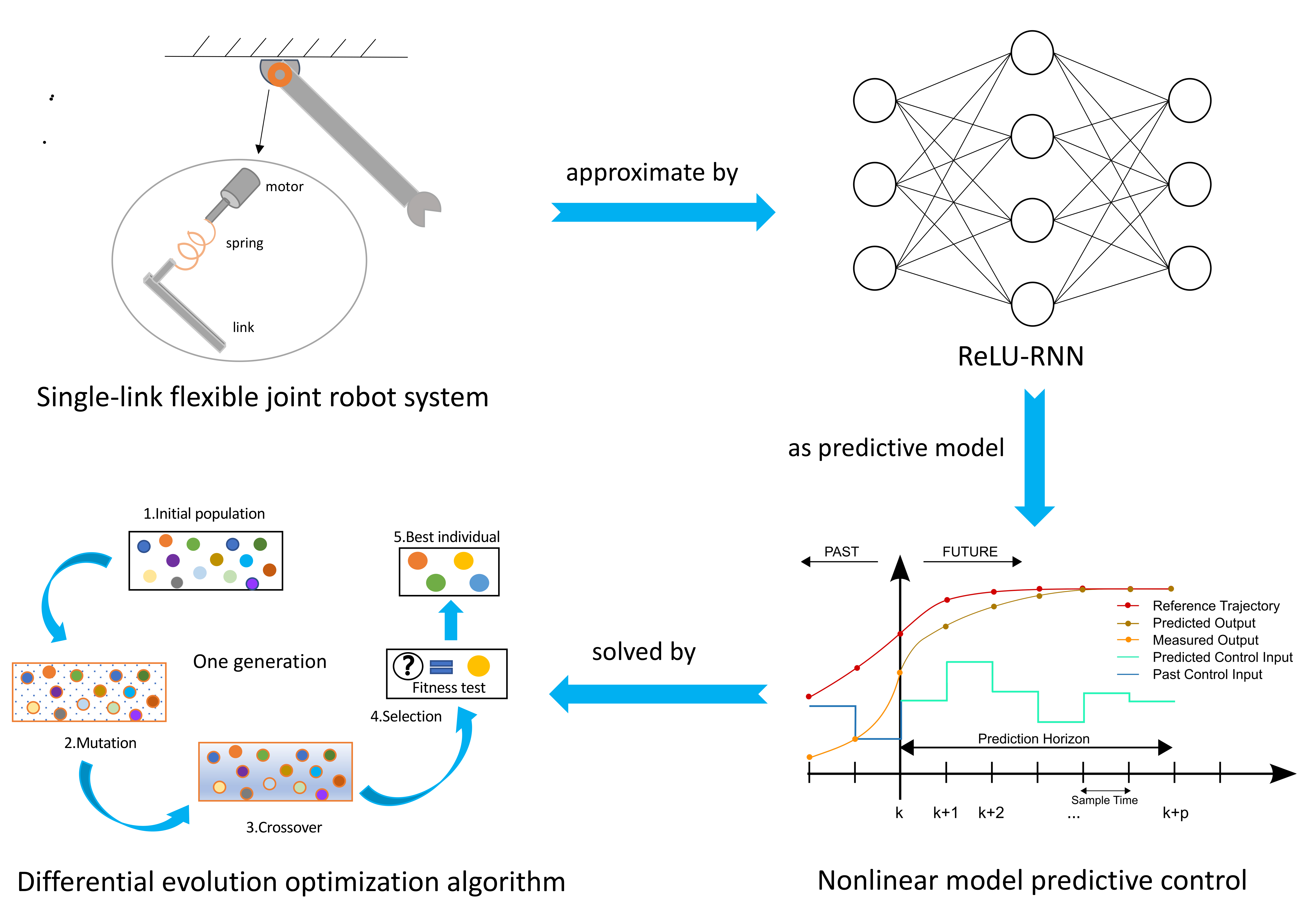
- To overcome the difficulty of modeling, a simple three-layer RNN with leaky rectified linear units as an activation function (ReLU-RNN) is established to approximate the FJ robot dynamic model with satisfactory precision. Then, according to the RNN predictive model and MPC approach, an RNN and DEO based NMPC controller is designed, in which the DEO algorithm is applied to solve the controller.
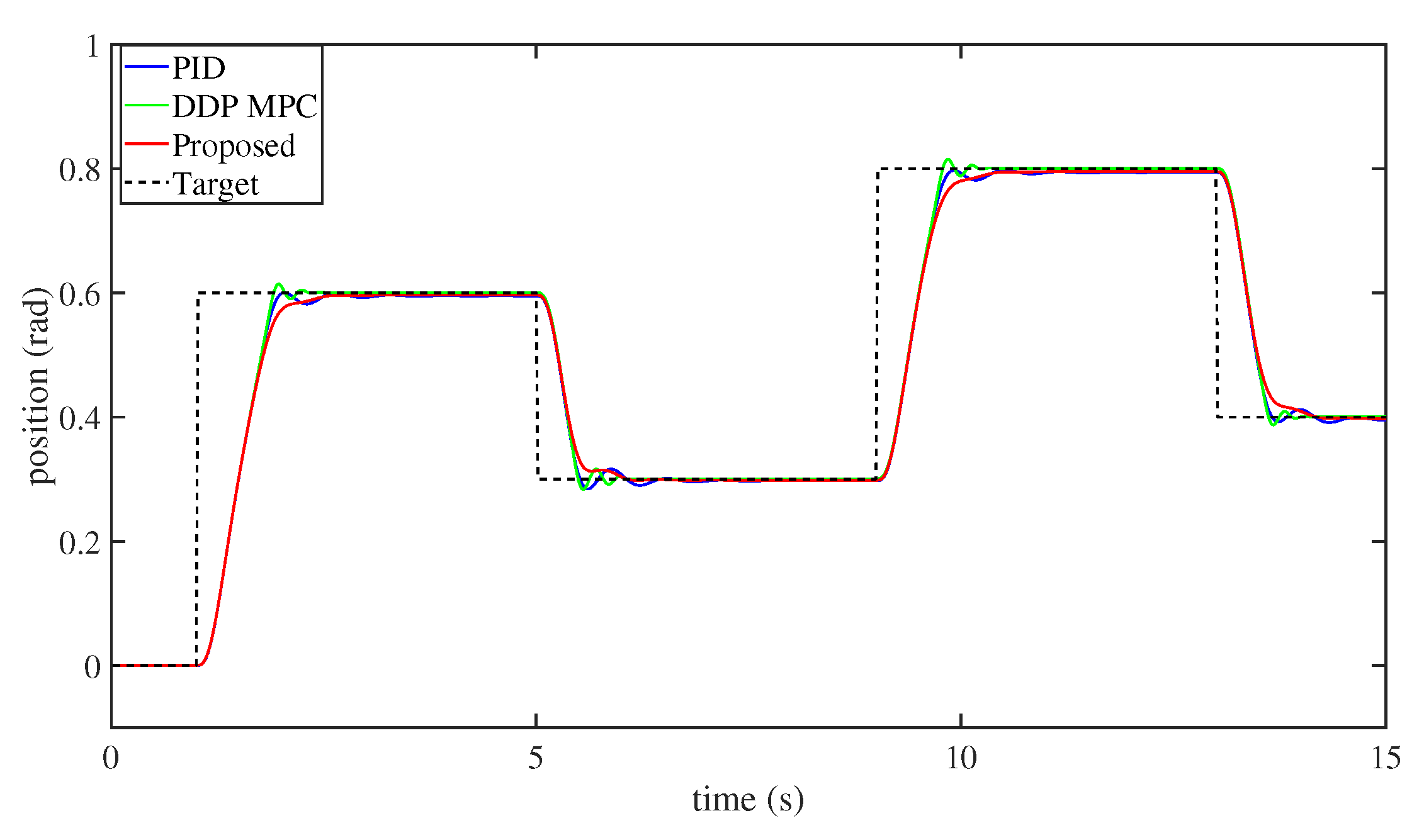
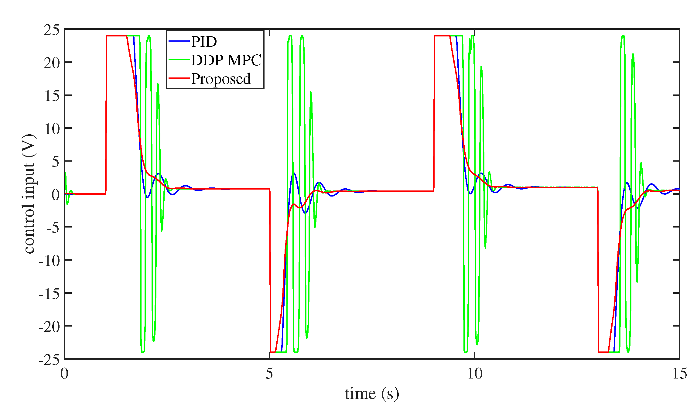
- Finally, to demonstrate the efficiency and performance of this technique, some numerical simulation comparisons between our method and the PD method and the differential dynamic programming (DDP) [57] MPC approach have been established. Numerical simulation findings illustrate that the performance of this technique is superior to that of the PD and DDP MPC methods.
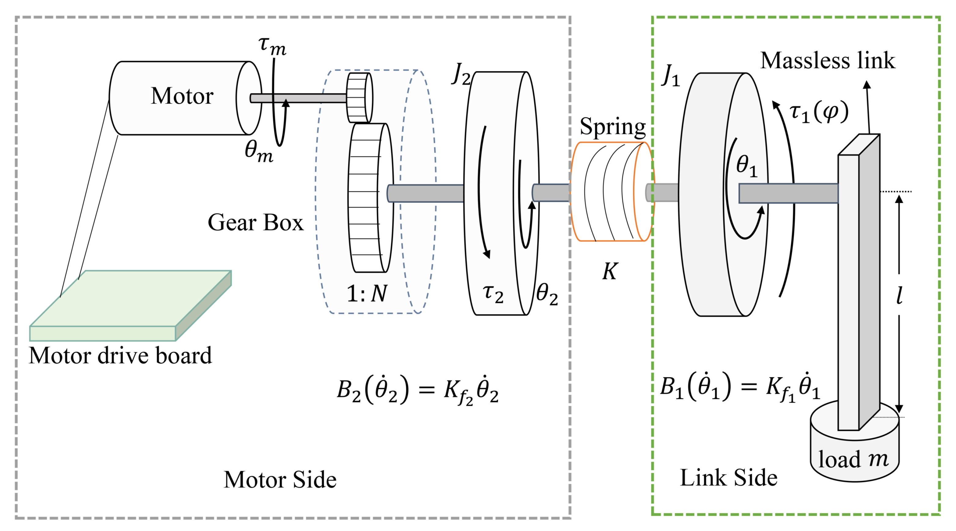
2. Single-Link FJ Robot System Model
3. Controller Design
3.1. Nonlinear Model Predictive Control
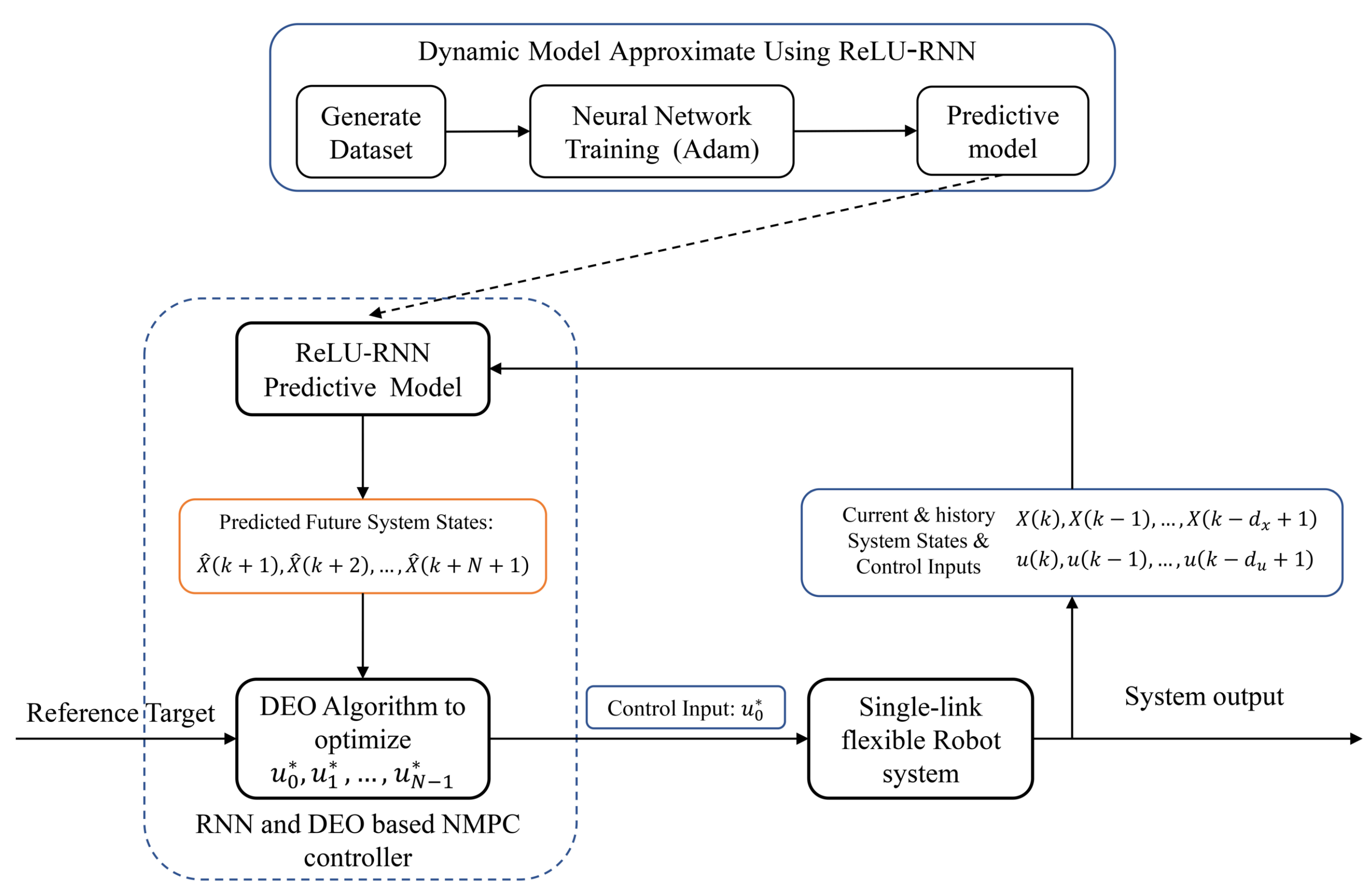
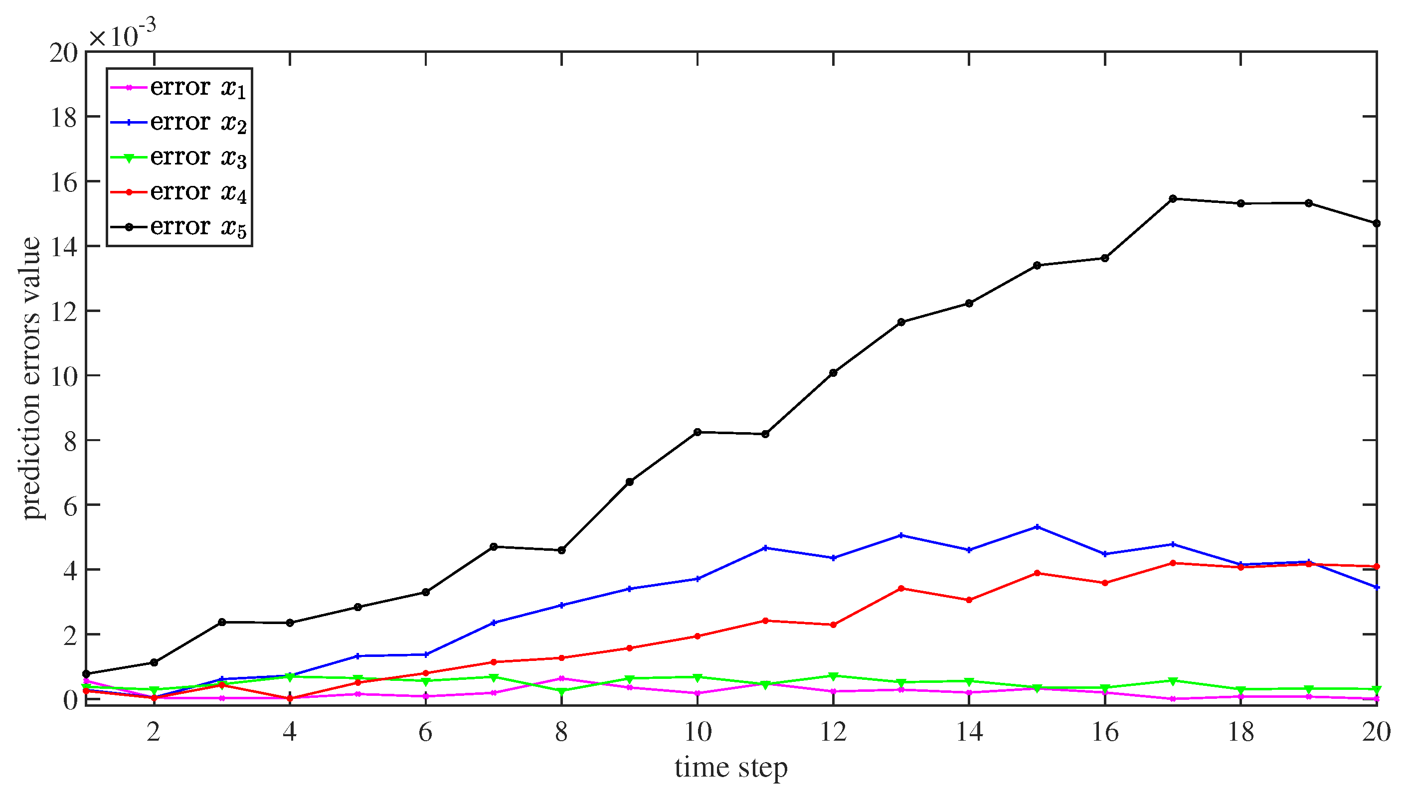
3.2. Dynamics Model Approximation Using ReLU-RNN
3.3. RNN and DEO Based NMPC Controller
- (1)
- DE/rand/1/bin
- (2)
- DE/rand/2/bin
- (3)
- DE/best/1/bin
- (4)
- DE/best/2/bin
- (5)
- DE/current-to-best/1/bin
- (6)
- DE/rand-to-best/1/bin
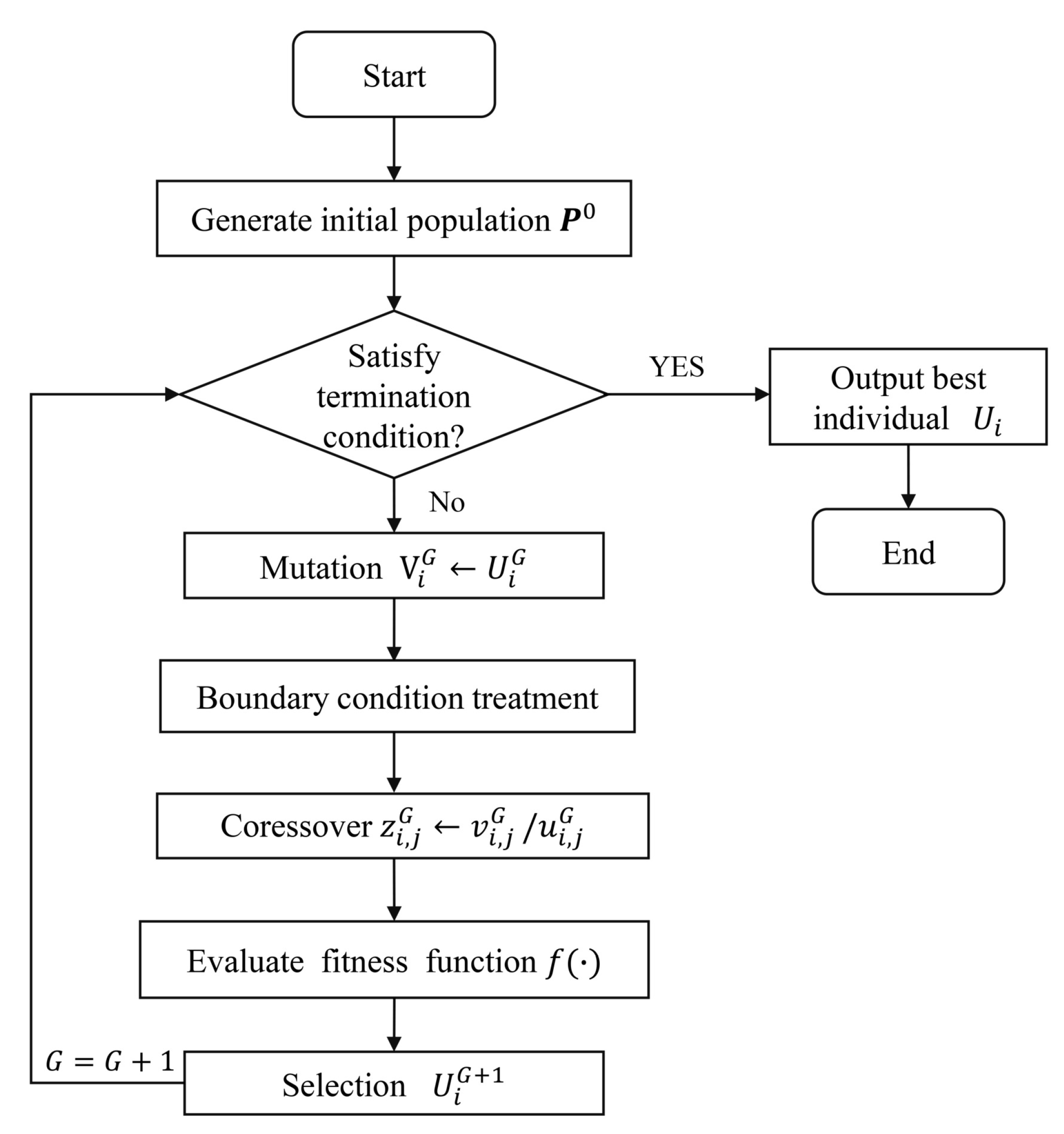
| Algorithm 1 The optimization process of DEO. |
Input:
|
- Step1.
- Obtaining the current system states and the saved history system states information along with system control inputs from the single-link flexible joint robot system.
- Step2.
- Based on the system state information, using the ReLU-RNN predictive model to predict future position states with N time steps.
- Step3.
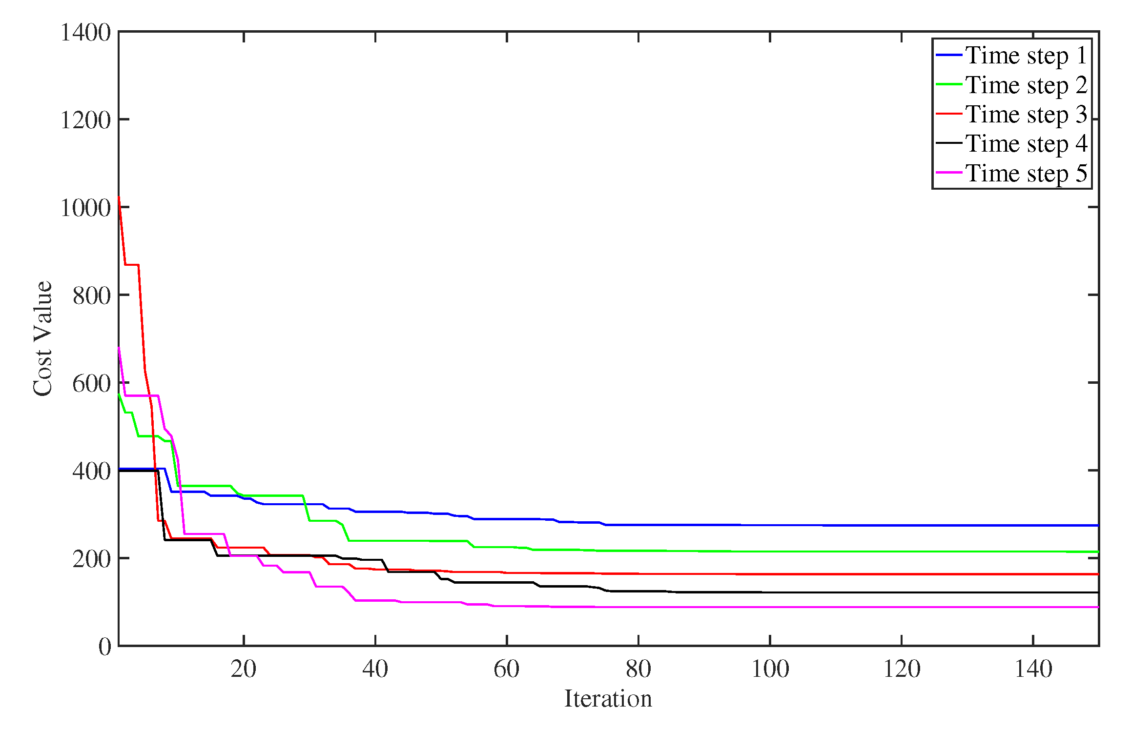
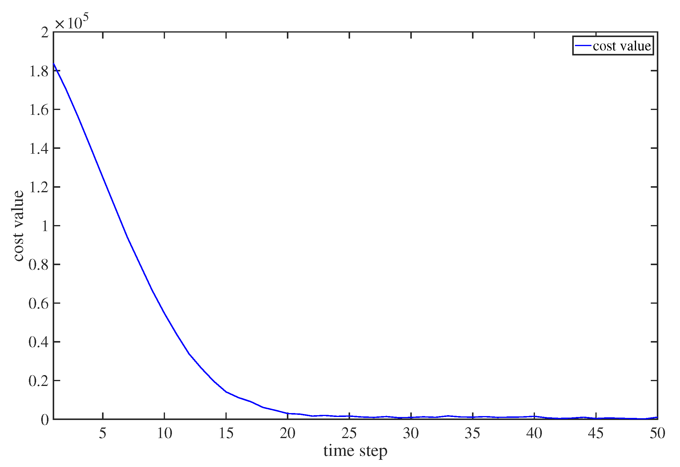
- According to the predicted system state information and the designed cost function, using the DEO (Algorithm 1) to solve the NMPC controller.
- Step4.
- Applying the first term () of the optimized control inputs to the system until the next time step.
- Step5.
- Time step proceeds forward one step (). Then, it updates the saved history system state information, and returns to Step 1.
3.4. Control Stability Analysis
4. Numerical Simulations
5. Conclusions
Author Contributions
Funding
Conflicts of Interest
References
- Spong, M.W. Adaptive control of flexible joint manipulators. Syst. Control Lett. 1989, 13, 15–21. [Google Scholar] [CrossRef]
- Brogliato, B.; Ortega, R.; Lozano, R. Global tracking controllers for flexible-joint manipulators: A comparative study. Automatica 1995, 31, 941–956. [Google Scholar] [CrossRef]
- Kim, M.S.; Lee, J.S. Adaptive tracking control of flexible-joint manipulators without overparametrization. J. Robot. Syst. 2004, 21, 369–379. [Google Scholar] [CrossRef]
- Huang, A.C.; Chen, Y.C. Adaptive sliding control for single-link flexible-joint robot with mismatched uncertainties. IEEE Trans. Control Syst. Technol. 2004, 12, 770–775. [Google Scholar] [CrossRef]
- Ibrir, S.; Xie, W.F.; Su, C.Y. Observer-based control of discrete-time Lipschitzian non-linear systems: Application to one-link flexible joint robot. Int. J. Control 2005, 78, 385–395. [Google Scholar] [CrossRef]
- Akyuz, I.H.; Yolacan, E.; Ertunc, H.M.; Bingul, Z. PID and state feedback control of a single-link flexible joint robot manipulator. Proceedings of 2011 IEEE International Conference on Mechatronics, Istanbul, Turkey, 13–15 April 2011; pp. 409–414. [Google Scholar]
- Liu, X.; Yang, C.; Chen, Z.; Wang, M.; Su, C.Y. Neuro-adaptive observer based control of flexible joint robot. Neurocomputing 2018, 275, 73–82. [Google Scholar] [CrossRef] [Green Version]
- Yin, W.; Sun, L.; Wang, M.; Liu, J. Nonlinear state feedback position control for flexible joint robot with energy shaping. Robot. Auton. Syst. 2018, 99, 121–134. [Google Scholar] [CrossRef]
- Wang, M.; Sun, L.; Yin, W.; Dong, S.; Liu, J. A novel sliding mode control for series elastic actuator torque tracking with an extended disturbance observer. In Proceedings of the 2015 IEEE International Conference on Robotics and Biomimetics (ROBIO), Zhuhai, China, 6–9 December 2015; pp. 2407–2412. [Google Scholar]
- Sun, L.; Yin, W.; Wang, M.; Liu, J. Position control for flexible joint robot based on online gravity compensation with vibration suppression. IEEE Trans. Ind. Electron. 2017, 65, 4840–4848. [Google Scholar] [CrossRef]
- Tomei, P. A simple PD controller for robots with elastic joints. IEEE Trans. Automat. Control 1991, 36, 1208–1213. [Google Scholar] [CrossRef]
- De Luca, A.; Siciliano, B.; Zollo, L. PD control with on-line gravity compensation for robots with elastic joints: Theory and experiments. Automatica 2005, 41, 1809–1819. [Google Scholar] [CrossRef]
- Alvarez-Ramirez, J.; Cervantes, I. PID regulation of robot manipulators with elastic joints. Asian J. Control 2003, 5, 32–38. [Google Scholar] [CrossRef]
- De Luca, A.; Flacco, F. A PD-type regulator with exact gravity cancellation for robots with flexible joints. In Proceedings of the 2011 International Conference on Robotics and Automation (ICRA), Shanghai, China, 9–13 May 2011; pp. 317–323. [Google Scholar]
- Albu-Schäffer, A.; Petit, C.O.F. Energy shaping control for a class of underactuated euler-lagrange systems. In Proceedings of the 10th IFAC Symposium on Robot Control, Dubrovnik, Croatia, 5–7 September 2012; Springer: Berlin/Heidelberg, Germany, 2012; Volume 45, pp. 567–575. [Google Scholar]
- Ju, J.; Zhao, Y.; Zhang, C.; Liu, Y. Vibration suppression of a flexible-joint robot based on parameter identification and fuzzy PID control. Algorithms 2018, 11, 189. [Google Scholar] [CrossRef] [Green Version]
- Tang, Q.; Chu, Z.; Qiang, Y.; Wu, S.; Zhou, Z. Trajectory tracking of robotic manipulators with constraints based on model predictive control. In Proceedings of the 17th International Conference on Ubiquitous Robots (UR), Kyoto, Japan, 22–26 June 2020; pp. 23–28. [Google Scholar]
- Wilson, J.; Charest, M.; Dubay, R. Non-linear model predictive control schemes with application on a 2 link vertical robot manipulator. Robot. Comput.-Integr. Manuf. 2016, 41, 23–30. [Google Scholar] [CrossRef]
- Carron, A.; Arcari, E.; Wermelinger, M.; Hewing, L.; Hutter, M.; Zeilinger, M.N. Data-driven model predictive control for trajectory tracking with a robotic arm. IEEE Robot. Autom. Lett. 2019, 4, 3758–3765. [Google Scholar] [CrossRef] [Green Version]
- Poignet, P.; Gautier, M. Nonlinear model predictive control of a robot manipulator. In Proceedings of the 6th International Workshop on Advanced Motion Control. Proceedings (Cat. No.00TH8494), Nagoya, Japan, 30 March–1 April 2000; pp. 401–406. [Google Scholar]
- De Nicolao, G.; Magni, L.; Scattolini, R. Robust predictive control of systems with uncertain impulse response. Automatica 1996, 32, 1475–1479. [Google Scholar] [CrossRef]
- Magni, L.; Sepulchre, R. Stability margins of nonlinear receding-horizon control via inverse optimality. Syst. Control Lett. 1997, 32, 241–245. [Google Scholar] [CrossRef]
- Mayne, D.Q.; Rawlings, J.B.; Rao, C.V.; Scokaert, P.O. Constrained model predictive control: Stability and optimality. Automatica 2000, 36, 789–814. [Google Scholar] [CrossRef]
- Hewing, L.; Wabersich, K.P.; Menner, M.; Zeilinger, M.N. Learning-based model predictive control: Toward safe learning in control. Annu. Rev. Control Robot. Auton. Syst. 2020, 3, 269–296. [Google Scholar] [CrossRef]
- Guo, K.; Pan, Y.; Yu, H. Composite learning robot control with friction compensation: A neural network-based approach. IEEE Trans. Ind. Electron. 2019, 66, 7841–7851. [Google Scholar] [CrossRef]
- Liu, X.; Zhao, F.; Ge, S.S.; Wu, Y.; Mei, X. End-effector force estimation for flexible-joint robots with global friction approximation using neural networks. IEEE Trans. Ind. Inform. 2019, 15, 1730–1741. [Google Scholar] [CrossRef]
- Liu, Y.J.; Li, J.; Tong, S.; Chen, C.L.P. Neural network control-based adaptive learning design for nonlinear systems with full-state constraints. IEEE Trans. Neural Netw. Learn. Syst. 2016, 27, 1562–1571. [Google Scholar] [CrossRef] [PubMed]
- He, W.; Chen, Y.; Yin, Z. Adaptive neural network control of an uncertain robot with full-state constraints. IEEE Trans. Cybern. 2016, 46, 620–629. [Google Scholar] [CrossRef] [PubMed]
- He, W.; Yan, Z.; Sun, Y.; Ou, Y.; Sun, C. Neural-learning-based control for a constrained robotic manipulator with flexible joints. IEEE Trans. Neural Netw. Learn. Syst. 2018, 29, 5993–6003. [Google Scholar] [CrossRef] [PubMed]
- Bai, G.; Meng, Y.; Liu, L.; Luo, W.; Gu, Q.; Liu, L. Review and comparison of path tracking based on model predictive control. Electronics 2019, 8, 1077. [Google Scholar] [CrossRef] [Green Version]
- Lenz, I.; Knepper, R.A.; Saxena, A. DeepMPC: Learning deep latent features for model predictive control. In Proceedings of the Robotics: Science and Systems XI, Rome, Italy, 13–17 July 2015. [Google Scholar]
- Gillespie, M.T.; Best, C.M.; Townsend, E.C.; Wingate, D.; Killpack, M.D. Learning nonlinear dynamic models of soft robots for model predictive control with neural networks. In Proceedings of the 2018 International Conference on Soft Robotics (RoboSoft), Livorno, Italy, 24–28 April 2018; pp. 39–45. [Google Scholar]
- Hyatt, P.; Wingate, D.; Killpack, M.D. Model-based control of soft actuators using learned non-linear discrete-time models. Front. Robot. AI 2019, 6, 22. [Google Scholar] [CrossRef] [Green Version]
- Hyatt, P.; Killpack, M.D. Real-time nonlinear model predictive control of robots using a graphics processing unit. IEEE Robot. Autom. Lett. 2020, 5, 1468–1475. [Google Scholar] [CrossRef]
- Li, D.; Li, D. Adaptive neural tracking control for an uncertain state constrained robotic manipulator with unknown time-varying delays. IEEE Trans. Syst. Man Cybern. Syst. 2018, 48, 2219–2228. [Google Scholar] [CrossRef]
- Karg, B.; Lucia, S. Efficient representation and approximation of model predictive control laws via deep learning. IEEE Trans. Cybern. 2020, 50, 3866–3878. [Google Scholar] [CrossRef] [PubMed]
- Thuruthel, T.G.; Falotico, E.; Renda, F.; Laschi, C. Model-based reinforcement learning for closed-loop dynamic control of soft robotic manipulators. IEEE Trans. Robot. 2018, 35, 124–134. [Google Scholar] [CrossRef]
- Hu, Y.; Su, H.; Fu, J.; Karimi, H.R.; Ferrigno, G.; De Momi, E.; Knoll, A. Nonlinear model predictive control for mobile medical robot using neural optimization. IEEE Trans. Ind. Electron. 2020, 68, 12636–12645. [Google Scholar] [CrossRef]
- Cao, Y.; Huang, J.; Xiong, C. Single-layer learning-based predictive control with echo state network for pneumatic-muscle-actuators-driven exoskeleton. IEEE Trans. Cogn. Dev. Syst. 2021, 13, 80–90. [Google Scholar] [CrossRef]
- Kumar, S.S.P.; Tulsyan, A.; Gopaluni, B.; Loewen, P. A deep learning architecture for predictive control. In Proceedings of the 10th IFAC Symposium on Advanced Control of Chemical Processes ADCHEM, Shenyang, China, 25–27 July 2018; pp. 512–517. [Google Scholar]
- Damasceno, B.C.; Xie, X. Deadlock-free scheduling of manufacturing systems using petri nets and dynamic programming. In Proceedings of the 14th IFAC World Congress 1999, Beijing, China, 5–9 July 1999; pp. 4870–4875. [Google Scholar]
- Fahmy, S.; Balakrishnan, S.; ElMekkawy, T. Deadlock prevention and performance oriented supervision in flexible manufacturing cells: A hierarchical approach. Robot. Comput.-Integr. Manuf. 2011, 27, 591–603. [Google Scholar] [CrossRef]
- Foumani, M.; Gunawan, I.; Smith-Miles, K. Resolution of deadlocks in a robotic cell scheduling problem with post-process inspection system: Avoidance and recovery scenarios. In Proceedings of the 2015 IEEE International Conference on Industrial Engineering and Engineering Management (IEEM), Singapore, 6–9 December 2015; pp. 1107–1111. [Google Scholar]
- Storn, R.; Price, K. Differential evolution-a simple and efficient adaptive scheme for global optimization over continuous spaces. J. Glob. Optim. 1997, 11, 341–359. [Google Scholar] [CrossRef]
- Tasoulis, D.K.; Pavlidis, N.G.; Plagianakos, V.P.; Vrahatis, M.N. Parallel differential evolution. In Proceedings of the 2004 Congress on Evolutionary Computation, Portland, OR, USA, 19–23 June 2004; Volume 2, pp. 2023–2029. [Google Scholar]
- Wang, H.; Rahnamayan, S.; Wu, Z. Parallel differential evolution with self-adapting control parameters and generalized opposition-based learning for solving high-dimensional optimization problems. J. Parallel Distrib. Comput. 2013, 73, 62–73. [Google Scholar] [CrossRef]
- Pedroso, D.M.; Bonyadi, M.R.; Gallagher, M. Parallel evolutionary algorithm for single and multi-objective optimisation: Differential evolution and constraints handling. Appl. Soft Comput. 2017, 61, 995–1012. [Google Scholar] [CrossRef]
- Zibin, P. Performance analysis and improvement of parallel differential evolution. arXiv 2021, arXiv:2101.06599. [Google Scholar]
- Opara, K.R.; Arabas, J. Differential evolution: A survey of theoretical analyses. Swarm Evol. Comput. 2019, 44, 546–558. [Google Scholar] [CrossRef]
- Al-Dabbagh, R.D.; Kinsheel, A.; Mekhilef, S.; Baba, M.S.; Shamshirband, S. System identification and control of robot manipulator based on fuzzy adaptive differential evolution algorithm. Adv. Eng. Softw. 2014, 78, 60–66. [Google Scholar] [CrossRef]
- Zhang, B.; Sun, X.; Liu, S.; Deng, X. Adaptive differential evolution-based receding horizon control design for multi-UAV formation reconfiguration. Int. J. Control Autom. 2019, 17, 3009–3020. [Google Scholar] [CrossRef]
- Jhang, J.Y.; Lin, C.J.; Young, K.Y. Cooperative carrying control for multi-evolutionary mobile robots in unknown environments. Electronics 2019, 8, 298. [Google Scholar] [CrossRef] [Green Version]
- Chen, C.H.; Lin, C.J.; Jeng, S.Y.; Lin, H.Y.; Yu, C.Y. Using ultrasonic sensors and a knowledge-based neural fuzzy controller for mobile robot navigation control. Electronics 2021, 10, 466. [Google Scholar] [CrossRef]
- Guo, H.; Cao, D.; Chen, H.; Sun, Z.; Hu, Y. Model predictive path following control for autonomous cars considering a measurable disturbance: Implementation, testing, and verification. Mech. Syst. Signal Process. 2019, 118, 41–60. [Google Scholar] [CrossRef]
- Gul, N.; Kim, S.M.; Ahmed, S.; Khan, M.S.; Kim, J. Differential evolution based machine learning scheme for secure cooperative spectrum sensing system. Electronics 2021, 10, 1687. [Google Scholar] [CrossRef]
- Wei, Y.; Wei, Y.; Sun, Y.; Qi, H.; Li, M. An advanced angular velocity error prediction horizon self-tuning nonlinear model predictive speed control strategy for PMSM system. Electronics 2021, 10, 1123. [Google Scholar] [CrossRef]
- MAYNE, B.D. A second-order gradient method for determining optimal trajectories of non-linear discrete-time systems. Int. J. Control 1966, 3, 85–95. [Google Scholar] [CrossRef]
- Slotine, J.J.E.; Li, W. Applied Nonlinear Control; Number 1; Prentice Hall: Englewood Cliffs, NJ, USA, 1991. [Google Scholar]
- Kingma, D.; Ba, J. Adam: A method for stochastic optimization. In Proceedings of the 2nd International Conference Learning Representations (ICLR), Banff, Canada, AB, 14–16 April 2014. [Google Scholar]
- Kwon, W.H.; Han, S.H. Receding Horizon Control: Model Predictive Control for State Models; Springer Science & Business Media: London, UK, 2006. [Google Scholar]
- Maciejowski, J.M. Predictive Control: With Constraints; Pearson Education Limited, Prentice Hall: London, UK, 2002. [Google Scholar]
- Storn, R. System design by constraint adaptation and differential evolution. IEEE Trans. Evol. Comput. 1999, 3, 22–34. [Google Scholar] [CrossRef] [Green Version]


| Parameters | Values | Parameters | Values |
|---|---|---|---|
| 0.8 kg· m | R | 5.3 | |
| 0.1 kg· m | 2.0 | ||
| N | 200 | 2.0 | |
| K | 70 Nm/rad | m | 0.3 kg |
| L | 1.4 × H | l | 0.5 m |
| 9.3 × Nm/A | g | 9.8 | |
| 0.1 V/rad/s | - | - |
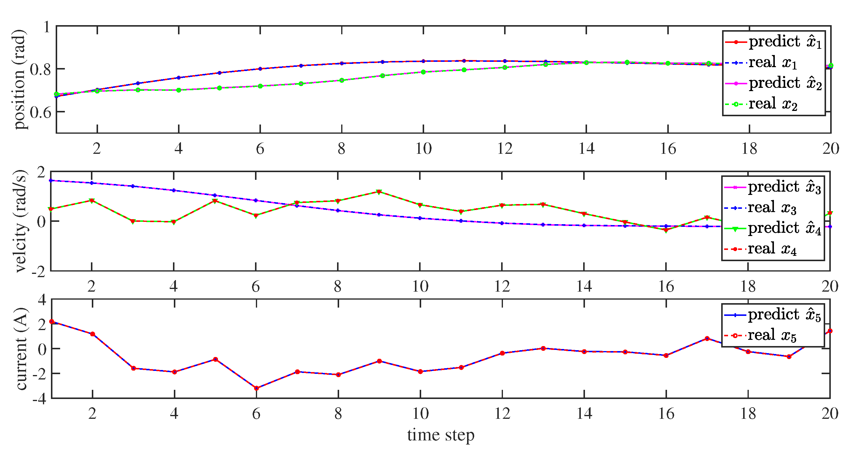
| States | (rad) | (rad/s) | (rad) | (rad/s) | (A) |
|---|---|---|---|---|---|
| MSE |
| Controller | Proposed | PID | DDP MPC |
|---|---|---|---|
| Proposed | 0.0037 | 0.0049 | 0.0016 |
Publisher’s Note: MDPI stays neutral with regard to jurisdictional claims in published maps and institutional affiliations. |
© 2021 by the authors. Licensee MDPI, Basel, Switzerland. This article is an open access article distributed under the terms and conditions of the Creative Commons Attribution (CC BY) license (https://creativecommons.org/licenses/by/4.0/).
Share and Cite
Zhang, A.; Lin, Z.; Wang, B.; Han, Z. Nonlinear Model Predictive Control of Single-Link Flexible-Joint Robot Using Recurrent Neural Network and Differential Evolution Optimization. Electronics 2021, 10, 2426. https://doi.org/10.3390/electronics10192426
Zhang A, Lin Z, Wang B, Han Z. Nonlinear Model Predictive Control of Single-Link Flexible-Joint Robot Using Recurrent Neural Network and Differential Evolution Optimization. Electronics. 2021; 10(19):2426. https://doi.org/10.3390/electronics10192426
Chicago/Turabian StyleZhang, Anlong, Zhiyun Lin, Bo Wang, and Zhimin Han. 2021. "Nonlinear Model Predictive Control of Single-Link Flexible-Joint Robot Using Recurrent Neural Network and Differential Evolution Optimization" Electronics 10, no. 19: 2426. https://doi.org/10.3390/electronics10192426
APA StyleZhang, A., Lin, Z., Wang, B., & Han, Z. (2021). Nonlinear Model Predictive Control of Single-Link Flexible-Joint Robot Using Recurrent Neural Network and Differential Evolution Optimization. Electronics, 10(19), 2426. https://doi.org/10.3390/electronics10192426