A Regularization-Based Big Data Framework for Winter Precipitation Forecasting on Streaming Data

Abstract

In the current paper, we propose a machine learning forecasting model for the accurate prediction of qualitative weather information on winter precipitation types, utilized in Apache Spark Streaming distributed framework. The proposed model receives storage and processes data in real-time, in order to extract useful knowledge from different sensors related to weather data. In following, the numerical weather prediction model aims at forecasting the weather type given three precipitation classes namely rain, freezing rain, and snow as recorded in the Automated Surface Observing System (ASOS) network. For depicting the effectiveness of our proposed schema, a regularization technique for feature selection so as to avoid overfitting is implemented. Several classification models covering three different categorization methods namely the Bayesian, decision trees, and meta/ensemble methods, have been investigated in a real dataset. The experimental analysis illustrates that the utilization of the regularization technique could offer a significant boost in forecasting performance.

1. Introduction

Widespread changes in the global distribution of living organisms, motivates the adequate monitoring of ecosystems that needs to be carried out at multiple scales. This will provide a robust scientific basis for decision making. Existing monitoring programs, either at small local scale or at large scale, that are set up to detect changes in biodiversity and ecosystem function, are rapidly evolving as new technologies arrive, but still lack key functionality [1]. Severe weather events can be exceptionally disastrous due to intense rainfall, tornadoes and wind storms that can occur over brief periods, frequently resulting in flash floods. The monitoring and the discovery of these climate occasions cannot decrease the quantity of these events, while an early warning can remarkably diminish the loss of life [2]. The techniques proposed in this work are based on the machine learning area and aim at classifying winter precipitation in an effective way.

As numerous developed countries have acquired sensor systems to identify precipitation along with life threatening and heavy storms, many areas are not covered by this kind of observation systems. Satellites can grant worldwide forecasts of rainfall, geostationary satellites offer coarser spatial resolution, while polar-orbiting satellites offer temporal coverage of storms with lower quality. Since catastrophic rainstorms can be developed within a few minutes and can last for some hours, sensor infrastructures need imperatively be deployed to effectively monitor such hazardous storms in a continuous way [3]. For regions that lack this kind of observation systems, it could be a literal lifesaver.

In particular, in the case of environment, a sensor network can automatically collect data directly related to weather conditions, air pollution, fire detection of forest areas or prevention of natural disasters. Moreover, using this kind of technology in the transportation sector, roads can be monitored via sensors; roads thus can be transformed and made smarter, safer, while traveler experience can be significantly improved. These sensor networks add further value to agriculture, where they can collect data and monitor different environmental conditions [4] such as the ones related to the microclimate in greenhouses, temperature, and soil moisture.

Forecast of winter precipitation has been consistently meliorating over the past two decades, despite the fact that there are still a plethora of inaccurate and uncertain estimates. All this significant progress technology has achieved, has permitted for advanced physics to be incorporated into models of expanding resolution.

Since precipitation is one of the foremost major climatic factors for ecosystem research, it contributes to weather forecasting, as well as climate monitoring. In spite of its significance, the accurate estimation of precipitation is still a most challenging problem. On the flip side of the coin, measurement errors for accurate precipitation, which are frequently ignored for automated frameworks, regularly range from $20\%$ to $50\%$ due to highly unpredictable wind conditions [5].

Despite the fact that measurement accuracy for precipitation can indeed be challenging to estimate and quantify, it is extremely vital for monitoring and evaluating climate variability and alternation. Diminishing uncertainties that regard measurement is fundamental, given the anticipated augmentations in precipitation over the following 100 year period.

Utilizing data from the U.S. Weather Surveillance Radar-1988 Doppler (WSR-88D) network, the Iowa Flood Center (IFC) has provided state-wide real-time precipitation information since the foundation of the IFC in 2009 [6]. This information was motivated by the requirement of real-time flood prediction in Iowa, a state which has repeatedly experienced devastating floods at different scales [7,8].

Large scale data are commonplace in applications and need a different handling in case of storing, indexing and mining. One well known method to facilitate large-scale distributed applications is MapReduce [9] proposed by Dean and Ghemawat. In order to address the above issues, many frameworks and distributed data-warehouses such as Hadoop, Spark, Storm, Flink, Cassandra and HBase are now quite well known and can be utilized as they process vast amounts of data efficiently. Additionally, there are libraries such as Spark’s MLlib, which are used in this article and which permit machine learning techniques in the cloud. There are also two different categories of Big Data processing, namely batch engines and streaming engines. The first is related to the management of a vast volume of data, while the second concerns the processing of high-velocity data. However, the most popular framework that manages large data environments for MapReduce batch processing is Hadoop. Recent applications require real-time analysis efficiently and effectively completed by streaming engines such as Spark and Storm Streaming [10].

In this study, given the difficulty or uncertainty in classifying winter precipitation [11,12], our objective is to develop a data-driven approach that can improve the accuracy of this particular classification problem. We have combined the data retrieved from the sensors so as to overcome the limitations of each radar-only method and have developed multiple classification models based on the supervised machine learning approach.

Collectively, to meet all the requirements and to address all the difficulties that arise in the work of classification in data streams, various methods are used, with the following being the most common:

• Bayesian methods, based on the Bayesian theorem with the algorithms (Bayesian classifiers) Naive Bayes and Multinomial Naive Bayes [13].
• Decision tree methods, which are the methods of decision trees with multiple variants and the main exponents of the algorithms Decision Stump [14], Hoeffding Tree (Very Fast Decision Trees) [15], Hoeffding Option Tree [16,17,18] and Hoeffding Adaptive Tree [19,20].
• Meta/ensemble methods, which are the combination of a set of classification models that perform the same task and the decisions of the individual models that are combined to decide the output to be produced. These methods are mainly implemented with the algorithms Bagging [21], Boosting [22], Bagging using Adwin [23], and Bagging using Adaptive-Size Hoeffding Trees.

The contribution of this present work is twofold. Primarily, the adoption of a cloud computing infrastructure in which Big Data technologies, such as Kafka, Spark Streaming and Cassandra, have been employed to develop an efficient schema for winter precipitation data storage and processing. Secondly, several classification models covering three different categorization methods, namely the Bayesian, Decision Trees and Meta/Ensemble methods and their performance in terms of accuracy metric and computation time, have been investigated in an extensive number of real data for different dataset sizes. Moreover, the classification performance was evaluated with and without the application of a regularization technique for feature selection; in this way, we can certainly avoid overfitting. As a final note, in our previous projects, the procedure of identifying and learning new data features while preserving old data ones can be considered as one of the most crucial goals of incremental learning methods [24,25].

The remainder of this paper is structured as follows. Section 2 presents information about real-time data processing systems, streaming, NoSQL databases, cloud computing infrastructures along with the classification algorithms used in the proposed approach and the regularization technique. Section 2.6 depicts the proposed architecture with the corresponding modules. In Section 2.7, the implementation system, the dataset and analysis of criteria are discussed, whereas in Section 3, the results are evaluated and presented in terms of tables along with the corresponding comparison. Recent scientific literature and various cloud computing methodologies are summarized in Section 4. Furthermore, Section 5 presents conclusions and draws directions for future work that may extend the current version and performance. Ultimately, the notation of this work is summarized in

Table 1. Article Notation.

Acronym	Explanation
ASOS	Automated Surface Observing System
WSR-88D	Weather Surveillance Radar-1988 Doppler
MLlib	Machine Learning library
NoSQL	Not-only Structured Query Language
VFDT	Very Fast Decision Tree
EWMA	Exponentially Weighted Moving Average
HAT	Hoeffding Adaptive Tree
Adwin	ADaptive WINdoing
Lasso	Least Absolute Shrinkage and Selection Operator
OLS	Ordinary Least Squares
NWP	Numerical Weather Prediction
Rain	RA
Freezing Rain	FRZA
Snow	SN
VM	Virtual Machine

.

2. Materials and Methods

This section describes the background theory associated with the foundations of our approach using tools and frameworks from computer science. In this study, we have employed a method for storage and processing of winter precipitation data using Big Data techniques that scale up and speed up winter precipitation data analysis and enhance weather forecasting. In particular, the adopted architecture is an integration of Apache Kafka, Spark and Cassandra. In the following subsections, we will give the necessary details of each component separately. Besides, useful knowledge about the considered classification models and regularization technique, the proposed architecture and, the experiments and data are described.

2.1. Apache Spark Streaming

Streaming data may be considered as the enormous amount of data/information addressed by a massive number of sensors and the shipment of those data records at the same time. These data need preparing a record-by-record premise to draw valuable and essential information. Moreover, the analytics can be sampled, filtered, correlated, or even aggregated, and this analysis can take place in a structure related to consumer aspects and a different business. Over time, stream processing algorithms are utilized with the goal of further refining the insights.

Apache Spark Streaming (https://spark.apache.org/streaming/ (accessed on 31 July 2021)) transforms the live input stream into batches, which are later on manipulated by Spark engine to produce the output in batches. Thus, D-streams consist of a high-level abstraction offered by Spark Streaming, whereas the latter grants the parallel processing of data streams by connecting to numerous data streams [26].

2.2. Apache Cassandra

Apache Cassandra (Retrieved July 31, 2021, from http://cassandra.apache.org/ (accessed on 31 July 2021)) consists of an open-source and widely scalable NoSQL (Not-only-SQL) database. Therefore, it is ideal for processing tremendous amounts of data in different data centers and a cloud infrastructure. One can consider the following features as its qualities, namely the persistent accessibility, the direct scalability, as well as the simplicity in operating on distinctive servers without any single point of failure [27].

Cassandra’s design is based on the premise that system and hardware failures occur consistently, and this fact results in a peer-to-peer distributed system. The information is distributed among all cluster nodes, whereas the replicating and sharing strategies are automatic and transparent. Moreover, it provides a progressed custom replication, which saves duplicates of the data on all nodes taking part in a Cassandra ring. If a node is shut down, then at least one copy of the node data will be available and accessible from another cluster node. Finally, Cassandra offers linear scaling capacity [28], which infers that the system’s overall capability can be immediately extended by including additional nodes to the network.

2.3. Apache Kafka

Apache Kafka (https://kafka.apache.org/ (accessed on 31 July 2021)) is an open-source distributed messaging system designed to process vast volumes of data. It is a distributed messaging system for collecting and transferring log files, integrated into Apache in 2011. To be precise, it is a system that transfers data from one application to another using a generalization of the messaging systems’ models. Thus, based on the queuing model, data processing is divided into a set of processes. In contrast, with the publish/subscribe model, Kafka allows the transmission of messages to a multitude of consumer groups [29].

The system is based on the Producer–Consumer model [30] and stores messages grouped into topics. A producer posts messages on a topic and the consumers who have registered in this topic receive the published message. Kafka implements four API types to connect with other applications. The first two are called Producer and Consumer, and are utilized for publishing feeds on one or more topics and showing interest in topics and processing data, respectively. The last two are the Streams and Connector APIs. The former is used for applications to act as data processors, while, the latter is used for creating reusable consumers or producers, and connecting topics with other applications or computer systems. For these reasons, Apache Kafka is an ideal solution for creating real-time pipelines and designing applications that process data streams.

2.4. Classification Algorithms

In the context of this section, useful details about the considered Machine Learning algorithms and techniques are given.

2.4.1. Naive Bayes

Naive Bayes is an algorithm known for its simplicity and low computational cost. It is useful for characterizing datasets with a high volume of information, as it runs efficiently and is easy to implement. As an incremental algorithm, it is suitable for application in feeds. However, we consider the features to be independent, which may not be possible in real feeds [13]. The Naive Bayes algorithm belongs to the Bayesian categorization methods, so it is based on the Bayes probability theorem and produces probability tables for each independent variable separately.

2.4.2. Decision Stump

The Decision Stump algorithm is a particular case of a decision tree belongs to the decision trees categorization method, where algorithms are used so as to construct trees as representations of results. It contains only one level of the decision tree, i.e., only one control node and two leaves; therefore, it can only predict two classes of the dependent variable [14]. It treats the missing values as different values and extends from the tree a third branch for these values. Finally, it is considered useful in two-class problems, although for the model to be built is quite simple.

2.4.3. Hoeffding Tree

In data streams, where not all data can be stored, the main problem with creating a decision tree is the need to reuse cases to calculate the best features. Domingos and Hulten proposed the Hoeffding Tree, or Very Fast Decision Tree (VFDT) [15], a Decision Tree algorithm waiting for new instances to arrive instead of using them again, which causes its rapid growth. This algorithm constructs a tree built from batch data with a substantial amount of them. Various extensions of the Hoeffding decision trees exist in the literature, some of which are used below. The variations aim to better deal with the “concept drift” and minimize the complexity of time and space.

2.4.4. HoeffdingOption Tree

The HoedffdingOption Tree algorithm extends the Hoeffding tree. The additional option nodes it contains allow multiple tests to be performed, resulting in separate paths and multiple Hoeffding trees [18]. The single structure of the option tree effectively represents many trees. The contribution of a specific example, which travels in different paths of a tree, can be done in many ways and with many varying options [16,17]. The main difference with the Hoeffding tree algorithm pseudocode is that each trainee can update instead of a single leaf, a group of option nodes, and there is a new method that is applied when a split is selected. If the unused feature is better than the current split, then the new option is introduced.

2.4.5. AdaHoeffdingOption Tree

The AdaHoeffdingOption Tree algorithm is an extension of a HoedffigOption Tree, an algorithm that could be interpreted as either a decision tree or an ensemble. In this method, it is not necessary to have a fixed size of the sliding window of data streams that change temporarily over time. A complicated parameter that users have to guess is the optimal size of the sliding window, which depends on the rate at which the distributed data changes [19].

The Adaptive Hoeffding Option Tree is a Hoeffding Option Tree that incorporates the following feature: adapts the Naive Bayes categorization to each leaf storing an estimation of the current error, while using an Exponentially Weighted Moving Average (EWMA) estimator with $\alpha$ = 0.2. In each voting process, there is a ratio of the weight of each node to the square of the inverse of the error [23].

2.4.6. HoeffdingAdaptive Tree

The HoeffdingAdaptive Tree or HAT algorithm extends the Hoeffding Window Tree by learning adaptive learning from the data stream. It adapts the Adwin (ADaptive WINdoing) algorithm [19]. Adwin solves the problem of detecting the average of real value numbers or a bit stream as it detects and evaluates changes. Moreover, it retains a set of recently passed variable-length instances. If there is no change in the average value in the window, it gains the maximum length [20]. It is used to monitor branches’ performance and replace them with new branches when their accuracy decreases if they are more accurate.

2.4.7. OzaBag

The OzaBag algorithm [22,31] belongs to the meta/ensemble classification methods, where combined classifiers can predict better than individual predictions. It is based on the Bagging algorithm [21], modified to apply to data streams. The term “bagging” is an abbreviation of “bootstrap aggregating”, where “bootstrap” is the method used to reproduce the training instances when the training set is small.

In the Bagging algorithm, an essential learning algorithm is used to extract the different M models that are potentially different because they are trained with varying bootstrap samples. Each sample is created by placing random samples from the original training set. The resulting meta-model predicts by taking a simple majority of the M classifiers’ predictions made in this way. The “Bagging” method, as stated by Breiman [32], does not seem to apply directly to feeds because it appears that the entire dataset is necessary to make bootstrap copies. The OzaBag algorithm shows how the bootstrap sampling process can be simulated in a data flow environment.

2.4.8. OzaBoost

The OzaBoost algorithm [22] belongs to the meta/ensemble classification methods and is based on the Boosting algorithm. In the Boosting algorithm, an essential learning algorithm is used to extract the different models trained with input samples, so as to achieve fewer errors. Unlike Bagging, models are created sequentially rather than in a parallel mode, and each new model is built according to the performance of previously constructed models. The main concern is to give more importance to the instances that have been wrongly sorted by the existing set of classifiers so that the next classifier in the sequence focuses on these instances.

For data flows, the OzaBoost algorithm was proposed. This algorithm uses a method that, instead of creating new models sequentially each time a new case arrives, updates each model with a weight calculated on previous classifiers’ performance. An essential function of the algorithm is to divide the total weight of the instances into two equal parts. The first part refers to the instances that are classified correctly, while the second refers to those that have been classified incorrectly. The Poisson distribution is used to determine the random probability that an instance will have to be used for training.

2.4.9. OzaBagAdwin

The OzaBagAdwin algorithm is an extension of the OzaBag algorithm that contains a drift detector, the Adwin algorithm [23]. The Adwin algorithm detects and evaluates changes in the results of the bagging method. If a change occurs, the less effective classifier is removed and a new one is added. In the process, the worst of the classifiers are immediately replaced with new base classifiers that have already been created.

2.5. Regularization Technique

Avoiding over-placement plays an essential role in training a machine learning model [33]. If the model is overfitting, it will have low accuracy as it tries to capture the training data set’s noise. The concept of noise refers to data points that do not represent the actual properties of the data, but random chance. The model is more flexible at the risk of over-placement, having previously learned such data points. The main difficulty with this kind of approach is finding the optimal balance. Therefore, various regularization parameter choice techniques have been proposed [34].

A challenging topic in the classification, is the feature selection as the minimum cardinality features are rarely known in advance. Adding more features to the set improves a predefined classification performance metric and accurately describes a given set of data. However, the classifier can be impeded by too many features.

$L1$ regularization or Lasso (Least Absolute Shrinkage and Selection Operator) Regression adds “absolute value of magnitude” of coefficient as penalty term to the loss function (L) and shrinks the less important feature’s coefficient to zero, thus removing some feature altogether [35]. According to Lasso, the penalized least squares regression with $L1$-penalty function is written as

$$Loss=\sum _{j=1}^m{(y_i-w_0-\sum _{i=1}^n{w}_i{x}_{ji})}^2+\lambda \sum _{i=1}^n\left|w_i\right|$$

(1)

where the value to be predicted is $y=w_0+w_1{x}_1+w_2{x}_2+\dots +w_n{x}_n$. The features that decide the value of y are $x_1,x_2,\dots ,x_n$; $w_0$ is the bias and $w_1,w_2,\dots ,w_n$ are the weights attached to $x_1,x_2,\dots ,x_n$, respectively.

In Equation (1), $\lambda$ is the regularization parameter that controls the importance of the regularization term. As a final note, if there is collinearity in the input values, Lasso regression method can perform effectively contrary to Ordinary Least Squares (OLS), which would overfit the data, a common method for parameter estimation.

In comparison with Ridge regression, also called $L2$ norm or regularization [36], Lasso shrinks the coefficient of less important features to zero, thus removing some features altogether. So, this works well for feature selection [37] in case we have a vast number of features. As a result, in the following, only the $L1$ regularization technique was implemented because the utilized dataset has only a limited number of features, and so, the expected accuracy will be the same for both strategies.

2.6. Proposed Architecture

2.6.1. Winter Precipitation Forecasting Model

Weather state forecasting has been crucial in various aspects of human life such as forestry, marine, agriculture and intelligent transportation for disaster prevention and emergency decision-making support [38]. For example, in the case of transportation, it concerns traffic flow prediction of autonomous vehicles in order to reduce traffic congestion and accidents, while in agriculture, it helps farmers to organize their work on any particular day.

A data-driven approach is employed to forecast the weather state based on winter precipitation, exploiting radar data related to several atmospheric variables. The model includes a number of meteorological and environmental data retrieved from various weather radars and a numerical weather prediction (NWP) model [39] (https://mesonet.agron.iastate.edu/request/download.phtml (accessed on 31 July 2021)).

The problem is treated as a classification task considering as target classes the weather conditions, namely, (1) rain (RA), (2) freezing rain (FRZA), and (3) snow (SN) according to an automated surface observing system (ASOS) [40]. Generally speaking, the weather classification model considers a set of n features based on temperature and precipitation. Here, we trained several machine learning models on every available sample of features and weather class label values $(d_{i1},d_{i2},\dots ,d_{in},c_i)$, where $c_i$ denotes the corresponding annotated weather class label of sample i. Then, we evaluated their classification performance based on the utilized model accuracy. More details are presented in the following sections.

2.6.2. Architecture Schema

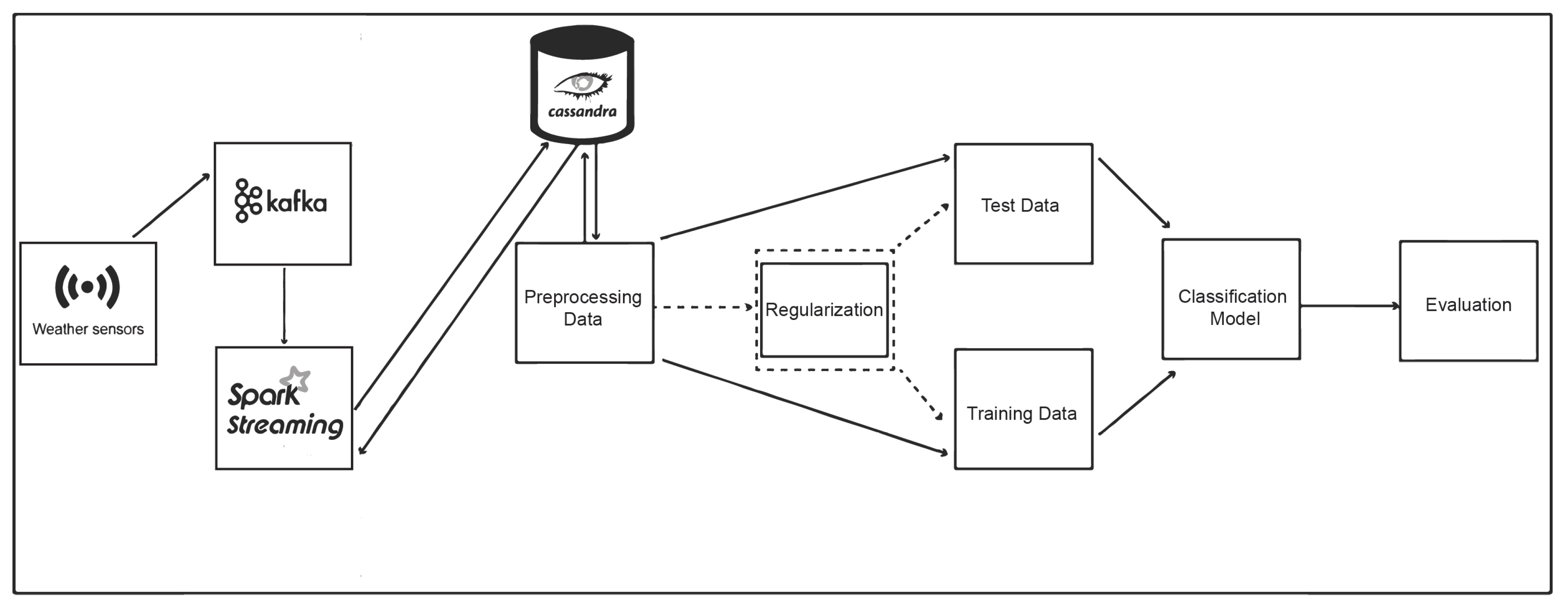
Our approach follows the proposal of knowledge discovery procedure as in [41]. First and foremost, we need to introduce the framework within which the computation took place. The overall architecture of the proposed system is depicted in Figure 1 taking into account the corresponding modules of our approach. Specifically, a pre-processing step is utilized and in following, the classification procedure is employed.

A novel system that consists of two main components, namely data collection and processing, is proposed in the present work. The data collection module, utilized with use of Apache Kafka, is developed to fetch the data from different weather sensors and, in following to store these data into Cassandra, a NoSQL database that is scheme-less and ideal for scalability purposes. After the storing procedure takes place, the system mainly performs real-time processing utilizing Apache Spark Streaming. Specifically, it is a data pipeline related to winter precipitation, which starts from a sensor that collects data. These data are then processed, stored, and analyzed. In more detail, the streaming pipeline can be analyzed in terms of the following aspects:

Weather sensors: the data that are given as input to our system in terms of weather data; some features are air temperature, dew point, wind speed, pressure altimeter, cloud coverage, and peak wind gust.

Apache Kafka and Apache Spark Streaming: these big data services are responsible for streaming and processing the data from sensors.

Cassandra: the data are stored in this particular NoSQL database in raw format and at a later stage, more refined information can be also stored as in [42].

Regularization Technique: this technique is implemented for feature selection in order to avoid overfitting. Specifically, as stated above, $L1$ regularization was employed.

Classification Procedure: nine classification algorithms, covering three different categorization methods, namely the Bayesian, the decision trees and meta/ensemble methods, have been investigated, and their performance in terms of accuracy metric and computation time has been evaluated.

2.7. Implementation

The proposed algorithmic framework has been implemented with the utilization of Apache Spark cloud infrastructure. The cluster used for our experiments includes 4 computing nodes, i.e., VMs, where each of them has four $2.5$ GHz CPU processors, 11 GB of memory and a 45 GB hard disk. One of the VMs is considered the master node and the other three VMs are used as the slave nodes.

2.8. Dataset

The dataset consists of variables associated with precipitation microphysics and the features are presented in

Table 2. Winter precipitation data description.

Variable	Description
station	Station Identifier (three or four characters)
valid	Observation Timestamp
tmpf	Air Temperature (Fahrenheit)
dwpf	Dew Point Temperature (Fahrenheit)
relh	Percentage of Relative Humidity
drct	Wind Direction in degrees from north
sknt	Wind Speed (knots)
p01i	One hour precipitation for the period from the observation time to the time of the previous hourly precipitation reset (inches)
alti	Pressure Altimeter (inches)
mslp	Sea Level Pressure (millibar)
vsby	Visibility (miles)
gust	Wind Gust (knots)
skyc1	Sky Level 1 Coverage
skyc2	Sky Level 2 Coverage
skyc3	Sky Level 3 Coverage
skyc4	Sky Level 4 Coverage
skyl1	Sky Level 1 Altitude (feet)
skyl2	Sky Level 2 Altitude (feet)
skyl3	Sky Level 3 Altitude (feet)
skyl4	Sky Level 4 Altitude (feet)
wxcodes	Present Weather Codes
feel	Apparent Temperature (Fahrenheit)
ice accretion 1 h	Ice Accretion over 1 h (inches)
ice accretion 3 h	Ice Accretion over 3 h (inches)
ice accretion 6 h	Ice Accretion over 6 h (inches)
peakwindgust	Peak Wind Gust (knots)
peakwinddrct	Wind Gust Direction (deg)
peakwindtime	Peak Wind Gust Time

[43,44]. The weather type is inferred by the precipitation classes as: (1) rain, (2) freezing rain, and (3) snow, as recorded in the automated surface observing system (ASOS) network, which were identified from the feature entitled wxcode. In this dataset, supervised learning by several classification models on streaming data will be applied.

For the training of the machine learning models, two approaches were considered. In the former, the models were trained considering all the available features as presented in Table 2, while in the latter, after the regularization technique, 13 features were selected and in following given as input.

In order to get an insight regarding the instances for each class, the percentages of data rows are depicted in

Table 3. Distribution of class instances.

Class	Percentage
Rain	$40\%$
Freezing Rain	$35\%$
Snow	$25\%$

. We can observe that the class “rain” has the highest percentage with value equal to $40\%$ while the percentages of “freezing rain” and “snow” are $35\%$ and $25\%$, respectively.

2.9. Criteria Analysis

As mentioned above, a corresponding dataset was used, consisting of a vast number of instances, as required for the correct evaluation of algorithms in the context of data flows. The 15 initial attributes are classified into two classes, whereas the separation of dataset to training and test set has been implemented with use of a cross validation procedure. The $80\%$ of the instances are used as a training set and the remaining $20\%$ as testing.

Accuracy is used as a measure of evaluation, defined as the ratio of all predictions that were correct to the total number of predictions. Each algorithm is evaluated for three different values of training instances with percentage of the training set equal to $80\%$, which are 80,000 (for 100,000 total instances), 200,000 (for 250,000 total instances) and 400,000 (for 500,000 total instances). For each algorithm, the percentage of accuracy is compared at specific moments, namely 500,000, 1,000,000, 5,000,000, and 10,000,000 processed instances. Moreover, another aspect that is taken into consideration concerns the relationships between the dataset size and the computation time needed to perform classification as well as between the dataset size and the metrics evolved.

Finally, nine classification algorithms were applied, as introduced in the previous subsection, which covers three different categorization methods, namely the Bayesian, the decision trees, and meta/ensemble methods. Another observation that needs to be taken into account is that in the OzaBag, OzaBoost, and OzaBagAdwin algorithms, the number of models used is ten, i.e., $M=10$, and the primary learning algorithm is the Hoeffding Tree.

3. Results

The results of our work are presented in

Table 4. Lowest, highest and average accuracy percentages of weather classification for dataset = 100,000.

Algorithm	Lowest	Highest	Difference	Average	Time
Classification without Regularization
Naive Bayes	74.25	79.50	5.25	77.08	0:24:45
Decision Stump	58.75	68.65	9.90	63.68	0:25:30
Hoeffding Tree	82.35	92.70	10.35	90.73	0:26:10
HoeffdingOption Tree	85.10	93.25	8.15	91.44	0:26:25
AdaHoeffdingOption Tree	83.05	93.00	9.95	91.28	0:26:35
HoeffdingAdaptive Tree	80.40	92.35	11.95	90.75	0:25:50
OzaBag	86.60	93.90	7.30	92.51	0:29:10
OzaBoost	88.10	93.45	5.35	91.92	0:28:40
OzaBagAdwin	86.75	93.85	7.10	92.51	0:28:30
Classification with Regularization
Naive Bayes	74.93	80.96	6.03	78.14	0:25:30
Decision Stump	60.15	69.86	9.71	64.82	0:26:30
Hoeffding Tree	83.26	93.18	9.92	91.16	0:28:00
HoeffdingOption Tree	85.81	94.39	8.58	92.53	0:28:15
AdaHoeffdingOption Tree	84.25	94.57	10.32	90.97	0:29:10
HoeffdingAdaptive Tree	80.54	92.15	11.63	91.35	0:28:50
OzaBag	85.83	94.19	8.36	93.63	0:29:55
OzaBoost	88.45	93.57	5.12	92.38	0:30:15
OzaBagAdwin	87.51	95.88	8.37	93.82	0:29:30

,

Table 5. Lowest, highest and average accuracy percentages of weather classification for dataset = 250,000.

Algorithm	Lowest	Highest	Difference	Average	Time
Classification without Regularization
Naive Bayes	76.16	78.44	2.28	77.08	0:43:35
Decision Stump	59.88	68.20	8.32	63.69	0:44:20
Hoeffding Tree	84.76	91.78	6.92	90.73	0:47:50
HoeffdingOption Tree	86.78	92.52	5.74	91.42	0:48:35
AdaHoeffdingOption Tree	85.92	92.26	6.34	91.28	0:48:20
HoeffdingAdaptive Tree	84.08	92.16	8.08	90.77	0:47:10
OzaBag	89.26	93.24	3.98	92.53	0:48:25
OzaBoost	89.76	92.78	3.02	91.92	0:48:35
OzaBagAdwin	89.22	93.22	4.00	92.51	0:47:50
Classification with Regularization
Naive Bayes	77.22	79.98	2.76	79.16	0:44:20
Decision Stump	60.56	71.27	10.71	67.73	0:45:25
Hoeffding Tree	85.82	92.55	6.73	91.42	0:49:30
HoeffdingOption Tree	86.96	94.77	7.81	92.94	0:50:15
AdaHoeffdingOption Tree	86.97	92.57	5.60	91.17	0:49:30
HoeffdingAdaptive Tree	84.84	92.95	8.11	91.28	0:50:35
OzaBag	90.20	93.82	3.62	92.91	0:50:40
OzaBoost	89.97	94.87	4.90	93.18	0:49:55
OzaBagAdwin	90.30	93.44	3.14	92.75	0:50:20

,

Table 6. Lowest, highest and average accuracy percentages of weather classification for dataset = 500,000.

Algorithm	Lowest	Highest	Difference	Average	Time
Classification without Regularization
Naive Bayes	76.39	77.84	1.45	77.08	0:55:20
Decision Stump	60.98	67.65	6.67	63.65	0:56:10
Hoeffding Tree	86.55	91.63	5.08	90.73	0:58:30
HoeffdingOption Tree	88.40	92.40	4.00	91.43	0:59:40
AdaHoeffdingOption Tree	87.59	92.19	4.60	91.28	0:58:55
HoeffdingAdaptive Tree	85.99	91.80	5.81	90.77	0:59:25
OzaBag	90.46	93.12	2.66	92.53	0:58:15
OzaBoost	90.29	92.52	2.23	91.93	0:58:40
OzaBagAdwin	90.54	93.10	2.56	92.51	0:59:20
Classification with Regularization
Naive Bayes	76.58	78.19	1.61	77.83	0:56:55
Decision Stump	62.56	67.96	5.40	65.65	0:57:40
Hoeffding Tree	86.94	93.55	6.61	92.24	1:00:15
HoeffdingOption Tree	88.91	93.49	4.58	92.96	1:00:20
AdaHoeffdingOption Tree	88.96	93.17	4.21	91.52	1:00:25
HoeffdingAdaptive Tree	87.22	93.89	6.67	92.58	0:59:30
OzaBag	90.81	94.44	3.63	93.84	1:01:15
OzaBoost	90.42	92.96	2.54	92.15	0:59:50
OzaBagAdwin	90.50	93.35	2.85	92.72	0:59:45

,

Table 7. Accuracy percentages of weather classification for different dataset sizes for training set $=\mathrm{80,000}$.

Algorithm	500,000	1,000,000	5,000,000	10,000,000
Classification without Regularization
Naive Bayes	76.10	76.95	76.80	78.35
Decision Stump	61.30	66.85	62.45	62.35
Hoeffding Tree	87.85	89.75	90.50	91.80
HoeffdingOption Tree	88.90	90.15	91.05	92.10
AdaHoeffdingOption Tree	88.65	89.80	91.10	91.80
HoeffdingAdaptive Tree	87.90	89.35	90.45	91.50
OzaBag	91.05	92.10	92.35	92.25
OzaBoost	90.25	91.80	92.00	91.80
OzaBagAdwin	90.95	92.10	93.00	93.00
Classification with Regularization
Naive Bayes	76.80	77.15	77.20	78.75
Decision Stump	61.87	66.78	62.76	63.14
Hoeffding Tree	88.19	90.28	91.93	92.75
HoeffdingOption Tree	89.18	90.75	91.85	93.35
AdaHoeffdingOption Tree	89.13	89.95	91.67	92.38
HoeffdingAdaptive Tree	88.45	89.87	90.92	92.67
OzaBag	91.67	92.85	93.35	93.85
OzaBoost	90.88	92.55	92.75	92.67
OzaBagAdwin	91.45	92.63	93.57	94.35

,

Table 8. Accuracy percentages of weather classification for different dataset sizes for training set = 200,000.

Algorithm	500,000	1,000,000	5,000,000	10,000,000
Classification without Regularization
Naive Bayes	76.26	76.52	77.64	77.16
Decision Stump	62.40	63.48	62.34	62.34
Hoeffding Tree	88.32	90.02	90.80	91.76
HoeffdingOption Tree	89.34	90.78	92.00	92.28
AdaHoeffdingOption Tree	88.86	90.40	91.64	92.16
HoeffdingAdaptive Tree	87.92	89.28	91.04	91.42
OzaBag	89.26	92.26	92.64	92.98
OzaBoost	89.76	91.76	92.70	92.08
OzaBagAdwin	89.22	92.28	92.50	92.88
Classification with Regularization
Naive Bayes	76.85	77.64	78.88	79.33
Decision Stump	62.93	63.65	63.14	63.76
Hoeffding Tree	89.19	90.78	91.76	92.37
HoeffdingOption Tree	90.05	91.65	92.35	92.88
AdaHoeffdingOption Tree	89.38	91.21	92.44	93.35
HoeffdingAdaptive Tree	88.34	89.57	91.69	92.33
OzaBag	90.45	92.63	93.32	93.85
OzaBoost	90.76	92.23	93.55	93.58
OzaBagAdwin	90.11	92.79	93.12	93.63

and

Table 9. Accuracy percentages of weather classification for different dataset sizes for training set = 400,000.

Algorithm	500,000	1,000,000	5,000,000	10,000,000
Classification without Regularization
Naive Bayes	77.15	76.71	77.13	77.15
Decision Stump	62.80	62.75	63.41	62.11
Hoeffding Tree	86.55	89.46	91.15	91.63
HoeffdingOption Tree	88.40	90.63	92.05	92.40
AdaHoeffdingOption Tree	87.59	90.37	91.83	92.19
HoeffdingAdaptive Tree	85.99	88.90	91.06	91.80
OzaBag	90.46	92.05	92.91	92.96
OzaBoost	90.29	91.56	92.51	92.38
OzaBagAdwin	90.54	92.04	92.85	92.87
Classification with Regularization
Naive Bayes	77.66	77.35	77.55	77.87
Decision Stump	63.45	63.75	64.14	63.98
Hoeffding Tree	87.87	90.55	92.17	92.82
HoeffdingOption Tree	89.05	91.15	93.24	93.88
AdaHoeffdingOption Tree	88.12	90.65	92.33	93.43
HoeffdingAdaptive Tree	87.12	89.45	92.62	93.54
OzaBag	91.55	92.77	93.78	94.43
OzaBoost	91.43	91.98	93.63	94.56
OzaBagAdwin	91.47	92.35	93.45	94.98

with and without the utilization of the regularization method described in Section 2.5. The accuracy metric evaluates each classifier’s performance in terms of different values, such as the lowest, highest, and average for different dataset sizes. The values of the accuracy depict the results based on the test set for each model. Furthermore, the training sets are differentiated in different tables to depict the variations in the accuracy metric. It is worth noting that the relation between the dataset size and computation time is not linear. For instance, for a dataset 5 times bigger, as it happens from 100 K rows to 500 K rows, we have to spend almost twice the computation time for the bigger dataset. We can observe that some classifiers outperform the others, and this pattern stands for all six tables.

3.1. Results for Different Training Set Values

The lowest, highest, and average percentages of accuracy for dataset equal to 100,000 rows (training set equal to 80,000) are presented in Table 4. Regarding classification without the utilized regularization technique, the lowest value is presented in the Decision Stump algorithm with a percentage of accuracy equal to 58.75%. In contrast, the largest value is presented in the OzaBag algorithm, with a percentage equal to 93.90%. We can observe that the difference between the lowest and highest percentages of accuracy in seven out of nine algorithms is below 10%. The most considerable value is presented in the HoeffdingAdaptive Tree, with a percentage equal to 11.95%. Moreover, in classification with regularization, the Decision Stump algorithm achieves the lowest value with a percentage of accuracy equal to 60.15% whereas, an immense value is shown in the OzaBagAdwin algorithm, with a percentage equal to 95.88%.

Moreover, Table 5 depicts the lowest, highest and average percentages of accuracy for dataset equal to 250,000 rows (training set equal to 200,000). The results are similar to Table 4, where Hoeffding, HoeffdingOption, AdaHoeffdingOption, and HoeffdingAdaptive Trees along with OzaBag, OzaBoost, and OzaBagAdwin achieve the highest accuracy values. For the classification without regularization, we can observe that the highest value is presented in the OzaBag algorithm with a percentage of accuracy equal to 93.24%. On the contrary, the lowest value is introduced in the Decision Stump algorithm, with a percentage equal to 59.88%. It is further depicted that the average values of accuracy in seven algorithms are over 90%. The most considerable value is presented in the OzaBag, with a percentage equal to 92.53%. Additionally, in classification with regularization, the highest value is shown in the OzaBoost algorithm with an average value equal to 94.87%. On the other hand, the lowest value is achieved in the Decision Stump algorithm, with a percentage equal to 60.56%.

Finally, results in Table 6 present the lowest, highest, and average percentages of accuracy for dataset equal to 500,000 rows (training set equal to 400,000). As in previous tables, the classifiers have almost the same performance, whereas the implementation of the regularization technique increases, as expected, the accuracy. Regarding classification without regularization, the Decision Stump algorithm achieves the lowest accuracy percentage, i.e., equal to 60.98%. In contrast, the most considerable value is shown in the OzaBagAdwin algorithm, with a percentage stretching to 90.54%. The difference between the lowest and highest percentage of accuracy in six algorithms is below $5\%$. The most considerable value is presented in the Decision Stump algorithm, with a percentage equal to 6.67%. Besides, in classification with regularization, seven algorithms have a percentage of accuracy over $90\%$. Simultaneously, the lowest value is given in the Decision Stump algorithm with a percentage of accuracy equal to 62.56%.

3.2. Results for Different Dataset Sizes

In Table 7, we observe that for a training set equal to 80,000, Naive Bayes and Decision Stump achieve the lowest accuracy values with the percentages equivalent to 78.35% and 62.35%, respectively. On the other hand, the OzaBagAdwin classifier has the highest accuracy with a percentage equal to $93\%$, followed by the OzaBag with a minimal difference of $0.75\%$. Moreover, in classification with regularization, the highest value is introduced in the OzaBagAdwin algorithm with a percentage of accuracy equal to 94.35%. Simultaneously, Naive Bayes and Decision Stump achieve the lowest accuracy values with percentages reaching 78.75% and 63.14%, respectively.

Table 8 presents the accuracy percentages for training set corresponding to 200,000. As in Table 7, Naive Bayes and Decision Stump have the lowest accuracy values with a percentage below $80\%$, whereas the other seven classifiers achieve almost the same performance, but the OzaBagAdwin classifier has the highest accuracy with a percentage equal to 92.88%. Regarding classification with regularization, we can observe that seven out of nine algorithms have a percentage over $92\%$. The most considerable value is presented in the OzaBag, with a percentage equal to 93.85%. On the other hand, the lowest value is depicted in the Decision Stump algorithm, with an accuracy percentage arriving to 63.76%.

Furthermore, the accuracy percentages for training set equal to 400,000 are presented in Table 9. As in previous Table 7 and Table 8, Naive Bayes and Decision Stump achieve the lowest accuracy values with percentages achieving 77.15% and 62.11%, respectively, while OzaBag and OzaBagAdwin perform slightly better than the remaining five classifiers with accuracy percentages equal to 92.96% and 92.87%, respectively. Moreover, in classification with regularization, the highest value is introduced in the OzaBagAdwin algorithm with an average value hitting 94.98%. On the other hand, the lowest value is achieved in the Decision Stump algorithm, with a percentage attaining 63.98%. In general, seven out of nine algorithms achieve almost the same performance having a percentage of over $92\%$.

3.3. Comparison

In the above experiments, a dataset of 10,000,000 rows was generated and nine classification algorithms were applied, covering three different categorization methods, namely the Bayesian, the decision trees, and meta/ensemble methods. Each algorithm was evaluated for three different instances of training sets, which are 80,000, 200,000, and 400,000, and the accuracy rate was examined in terms of the number of instances.

To sum up the results, we can see that the OzaBag, as well as OzaBagAdwin meta-algorithms, are the ones that achieve the highest accuracy. The proposed method with the regularization strategy performs slightly better than the classifiers without the utilization of any regularization strategy in terms of the accuracy metric. Specifically, we could say that the proposed method produced, in most cases, about $1\%$ more accurate results, whereas in some cases, the percentage is more than $2\%$. This is very important, as in most cases, the accuracy percentages already exceed values equal to $90\%$.

However, as expected, the proposed method does not clearly outperform the ground truth method for all nine classifiers because of the low number of dataset features. Furthermore, as the dataset increases, all classifiers perform better, and this is an indication that the proposed schema can be efficiently proposed in a real-time system measuring air quality streaming information.

4. Discussion

The area of data mining did not come into presence until recently when the expressed objective of systemizing the techniques and strategies for identifying hidden patterns, clustering [45,46] or other knowledge of interest [47,48] from massive datasets was introduced. Specifically, data mining offers the tools for extracting latent associations between characteristics and features, hence permitting feature transformation and dimensionality reduction [49]. The two above characteristics are considered mandatory in the extract-transform-load ($ETL$) cycle appearing in databases. A portion of applications that can be associated with knowledge discovery is finance, marketing, as well as fraud detection [41]. More to this point, the procedure of knowledge discovery is organized in numerous stages starting with the feature selection. In following, the pre-processing and transformation steps come into presence and finally, concluding with the main stage of data mining, an appropriate algorithm has the potential to extract latent information in a form suitable for future utilization [50].

Regarding big data architectures, authors in [51] suggest a real-time remote prediction system for health status, implemented on Apache Spark and deployed in the cloud, whose aim is to apply machine learning model on streaming Big Data. Bear in mind that Apache Spark is an open-source engine for Big Data processing. Moreover, machine learning for streaming data challenges (such as data pre-processing, dimensionality reduction, semi-supervised learning, ensemble learning, etc.) and opportunities are presented in detail in [52]. In [25], the singular value decomposition (SVD) performs attribute transformation and selection, and boosts the performance of various Spark MLlib classifiers in Kaggle datasets. In addition, a novel healthcare monitoring framework for chronic patients was presented in [53], which integrates advanced technologies, including data mining, cloud servers, big data, ontologies, and deep learning. The proposed framework enhances the performance of heterogeneous data handling and processing, and improves the accuracy of healthcare data classification.

There has also been increasing interest in sophisticated algorithms (e.g., machine learning) for low-cost sensor calibration in recent years. To date, there have been published studies using high-dimensional multi-response models [54] and neural networks [55,56]. In [55], excellent performance with dynamic neural network calibrations of NO${}_2$ sensors was demonstrated; however, the same performance for O${}_3$ was not observed.

Precipitation is one of the major fundamental factors in environmental and atmospheric sciences, which includes research related to weather and hydrology. Precipitation prediction is becoming more precise due to advanced remote-sensing technology and the presence of solid ground reference systems [57,58]. On the other hand, the evaluation of mixed precipitation remains challenging because the identification and the reliable measurement of numerous diverse types of precipitation remain highly difficult [5,59]. Information regarding this type of precipitation is vital in terms of the management of infrastructure and facility (e.g., air/ground traffic control, road closure) especially during the winter season in many areas [60].

Winter precipitation, in the form of freezing rain, sleet and snow, is a hazard that can have disruptive impact on human lives [60]. One of the most prominent effects of these forms is when traveling via vehicles and aircraft. Non-ideal road conditions or even reduced visibility during winter precipitation can lead to vehicle collisions, whereas flight through winter precipitation can lead to aircraft accidents.

The conventional way of monitoring winter weather types (e.g., snow and freezing rain) has often relied on the dual-polarization capability of weather radars, which allows us to define hydrometeor types [61]. Radar is indeed used to monitor for precipitation and even precipitation type, particularly with the dual-pol capability. However, automated surface observing system (ASOS) [40], other surface observations, satellite, short-term numerical models, objective analyses, and social media are also equally important in the monitoring of current precipitation type, rates, and coverage.

Recent studies regarding radar data analysis, have focused on machine learning methodologies for solving complex problems such as convective storm forecasting and quantitative precipitation estimation. In most cases, conventional rainfall prediction based on radars is implemented by known functional connections between the rainfall intensity and various radar measurements. Authors in [62] employed the utilization of two supervised machine learning strategies, namely random forest and regression tree in rainfall prediction, using dual polarization radar variables that do not have any predefined relationships. An approach using the temporal properties of the convective storms based on machine learning models for predicting future locations is introduced in [63].

Precipitation prediction is considered a principal issue with several environmental applications, such as flood monitoring and agricultural management. Specifically, authors in [64] proposed a deep learning model on a combination of precipitation radar images as well as wind velocity based on a weather forecast model for determining if using additional meteorological features like the wind would improve prediction.

The most critical challenge concerning data classification is that of “concept drift” [65]. The phenomenon of “concept drift” is caused by the natural tendency of data to naturally and uninterruptedly evolve over time. It is most likely that after a certain period, the classifier’s predictor accuracy will deteriorate due to the constant change of the flow of information. It is common knowledge that in real-world applications, data stem from non-stationary distributions resulting in the “concept drift” or “non-stationary learning” problem, often related to streaming data scenarios [66]. Finally, it should be noted that, in the current study, it is assumed that this phenomenon does not occur in the experimented data.

5. Conclusions and Future Work

This work focuses on two semantic aspects directly associated with distributed machine learning; the first one is the performance of classifiers with and without a regularization technique in terms of the accuracy metric, and the second one is the relation of the dataset size with this particular metric. In our proposed schema, to avoid overfitting and subsequently lower accuracy in our model, $L1$ regularization or Lasso Regression was employed. This technique adds as penalty term to the loss function (L) the “absolute value of magnitude” of coefficient and hence, shrinks the coefficient of less important features to zero, removing in this way a number of features altogether.

To test our approach, nine classification algorithms were applied, covering three different categorization methods, namely the Bayesian, the decision trees, and meta/ensemble methods. Each algorithm was evaluated for three different instances of training sets, which are 80,000, 200,000, and 400,000, and the accuracy rate was examined in terms of the number of instances.

Ultimately, the present work can introduce some particular findings and conclusions. Firstly, the potential of Spark Streaming to efficiently process a large amount of data and to seamlessly apply well-known machine learning operations to big data is shown. Additionally, it should be noted that the regularization technique provides an increase in classification accuracy, even in cases where accuracy already achieves high values. Third, from an algorithmic perspective, these hybrid architectures based on regularization techniques can be more effective specifically when considering a distributed infrastructure, and hence the performance of the system will be eventually increased.

Regarding future work, other concrete datasets can be utilized for further experimenting on the performance benchmarks of the proposed classification strategy. A better understanding of the optimal combinations between the size of features set and utilized classifiers will be achieved by implementing additional tests. Furthermore, neural network approaches can be employed to efficiently predict winter precipitation data as in [55,56]. Furthermore, the inefficiencies of single models can be resolved by applying several combination techniques, which will lead to more accurate results.