Abstract
The use of behavioral models based on deep learning (DL) to accelerate electromagnetic field computations has recently been proposed to solve complex electromagnetic problems. Such problems usually require time-consuming numerical analysis, while DL allows achieving the topologically optimized design of electromagnetic devices using desktop class computers and reasonable computation times. An unparametrized bitmap representation of the geometries to be optimized, which is a highly desirable feature needed to discover completely new solutions, is perfectly managed by DL models. On the other hand, optimization algorithms do not easily cope with high dimensional input data, particularly because it is difficult to enforce the searched solutions as feasible and make them belong to expected manifolds. In this work, we propose the use of a variational autoencoder as a data regularization/augmentation tool in the context of topology optimization. The optimization was carried out using a gradient descent algorithm, and the DL neural network was used as a surrogate model to accelerate the resolution of single trial cases in the due course of optimization. The variational autoencoder and the surrogate model were simultaneously trained in a multi-model custom training loop that minimizes total loss—which is the combination of the two models’ losses. In this paper, using the TEAM 25 problem (a benchmark problem for the assessment of electromagnetic numerical field analysis) as a test bench, we will provide a comparison between the computational times and design quality for a “classical” approach and the DL-based approach. Preliminary results show that the variational autoencoder manages regularizing the resolution process and transforms a constrained optimization into an unconstrained one, improving both the quality of the final solution and the performance of the resolution process.
1. Introduction
Recently, many research areas have benefited from the potential offered by deep learning (DL) tools, such as convolutional neural networks (CNNs) [1,2]. In fact, recent works on the DL-assisted analysis of electromagnetic (EM) field computation problems showed the promising potential of CNN applications [3,4,5,6,7,8,9,10,11,12,13,14,15].
The idea that properly trained DL models can substitute the direct calculation of Maxwell’s equations [3,14], or provide an end-to-end solution for the performance analysis of electric devices [5] is maturing in the community of computational electromagnetics. A comprehensive review of recent works on machine learning for the design optimization of electromagnetic devices can be found in [4], where the growing interest of the community for DL is clearly evidenced. Some works have adopted DL models to predict the key performance indicators of electrical machines [6,8,9,15], whilst others have focused on topology optimization [10,11,12,13].
The main application of most of the mentioned works is the optimization of the geometry of rotating electrical machines, in particular permanent magnet machines, in order to optimize an electromagnetic parameter such as maximizing the motor torque and/or minimizing the cogging torque. Some works have faced additional theoretical problems such as obtaining reduced models [9], or treating the optimization of special electromagnetic devices [7,10].
We acknowledge that the literature regarding the application of DL to the design and optimization of electromagnetic devices under low frequency is still relatively scarce, and in many works, it is difficult to find detailed information regarding used DL models, the size and number of hidden layers, the exact training algorithms used, the dimensions of the input and output patterns, the dataset size and the generation method. In this work, we try to give to the reader a detailed description of the models; in particular, we provide the complete pseudo-codes of the algorithms used for the training and optimization phases, and we also provide complete details regarding the models’ architectures and the generation of the dataset.
Among the DL models and architectures, autoencoders enjoy particular attention in applications where the high dimensional input space needs to be mapped and interpreted in a lower dimensional space, as in the case of complex geometries of electromagnetic devices [7,10]. Autoencoders can use fully connected and convolutional layers and perform nonlinear compression through the encoder network of the input space to a lower dimensional, called the latent space, and the compressed data can be decoded back (reconstructed) to the original space through the decoder network. This unsupervised learning architecture opens a number of possible applications:
- The latent space features can be used for design and optimization in a low-dimensional space;
- The reconstructed patterns represent a regularized and denoised version of the input patterns;
- In the form of a variational autoencoder the model can generate new data;
- The encoder can be trained in order to encode useful features for the optimization.
Among these, the third and particularly the fourth features are not exploited in the literature as much as the first two, and they represent one of the main motivations and contributions of this work. A variational autoencoder (VAE) [16,17] can be defined as being an autoencoder whose training is regularized to avoid overfitting and ensure that the latent space has good properties that enable a generative process. VAEs have a number of applications, from intrusion detection [18,19] to the prediction of lung cancer [20], and some works have employed VAEs and other generative models such as GANs (generative adversarial networks [21]) to aid in optimization [22,23,24].
1.1. Related Works
In previous works, authors have introduced various deep learning-based optimization algorithms [7,9,10], and their main characteristics are summarized in Table 1. In particular, in [10], a standard autoencoder was used to represent the input geometries of a special device as bitmaps, and the electromagnetic problem was optimized in the latent space using an evolutionary optimization algorithm. In [7,9], deep learning models were developed to represent both the geometry and the relationship between the geometry and the resulting electromagnetic fields, and the optimization was carried out using particle swarm optimization (PSO) [9] and a genetic optimization algorithm (GA) [7]. In the aforementioned works, particularly [7,10], the problem of obtaining a surrogate model to properly solve a given electromagnetic problem for different geometries was solved using two main DL models: namely a model to represent the input image in a reduced dimensional space, i.e., the latent space of the autoencoder; and a model to predict the electromagnetic variables (to be optimized) as a function of geometry, that we shall denote as a surrogate model (SM). The rationale of the SM is to substitute a costly finite element analysis (FEA) inside the optimization loop. Some critical aspects of previous works [7,10] can be evidenced, for example, the two DL models were separately trained without a regularization procedure, aiming to minimize different objectives: the reconstruction error for the autoencoder and the mean square error (MSE) for the SM. Moreover, geometry optimization was carried out using general purpose population-based optimization algorithms, which are very computationally expensive, necessitate explicitly managing the constraints and do not directly take into account the gradient of the objective function with respect to the geometry.

Table 1.
Main aspects of related works.
1.2. Main Features of the Proposed Model
In this work, a novel method based on a variational autoencoder is introduced, and the optimization is performed in the latent space generated by the VAE.
In particular, we consider the same application treated in [7], i.e., the TEAM 25 problem, consisting of the optimization of the geometry of an electromagnetic die press.
The main novelties of the proposed approach, with respect to previous ones, are the following:
- The variational autoencoder and the surrogate model were simultaneously trained in a custom multi-model training loop, aiming to minimize a combined loss function that includes a regularization term;
- The optimization of the geometry was carried out in the regularized latent space using gradient descent optimization, which is less computationally expensive than evolutionary optimization algorithms;
- The optimization process in the latent space is totally unconstrained, because the variational autoencoder only learns to map feasible solutions.
With respect to the latent space of a standard autoencoder, the latent space of a variational autoencoder is, in general, smooth and well behaved: data are represented in a continuous and convex space, which is particularly well suited for a gradient descent search. This result was obtained thanks to a regularization term that is at the base of the VAE learning process. Furthermore, we show that the simultaneous optimization of the surrogate model and the VAE allows two main results:
- The encoder parameters are influenced by the performance of the surrogate model, thus the VAE incorporates useful features for the optimization, generating a latent space that is well regularized and optimized for the good operation of the surrogate model;
- The training of the surrogate model is naturally regularized, avoiding overfitting, thanks to the regularization term of the VAE.
As a result, the subsequent gradient descent optimization in the latent space of the VAE is feasible, fast and accurate. In contrast to previously used population-based optimization approaches, the gradient descent optimization is based on a smooth and gradual progress that can easily reveal geometry features that are desired or undesired.
The nature of the proposed algorithm allows to efficiently deal with problems with a very high number of degrees of freedom. In fact, we are approaching the problem of topological optimization, where the search domain is represented with a bitmap and every pixel is a variable to be optimized. In standard parametric optimization, the geometry to be optimized is usually represented by a small number of parameters, such as a radius, segments or parameterized shape. In our case, the geometry can be chosen with more freedom, as each pixel can be freely selected to be full or empty (of ferromagnetic material). In particular, in our test case, we have 900 degrees of freedom. The efficiency of the algorithm is demonstrated by comparing its performance against other approaches, as reported in the results section.
This paper is organized as follows: in Section 2, we present the variational autoencoder and the custom training loop, as well as the autoencoder-based optimization loop. In Section 3, the selected test case (TEAM 25 problem) is introduced, the FEA model is detailed and a standard full FEA-based optimization is performed to be used as a comparison term. In Section 3, we also describe the basis of the bitmap geometry representation and introduce the generated dataset used to train the DL model. In Section 4, we perform the selection of model architecture and meta-parameters, and we test the trained DL model. In Section 5, we discuss the results and finally we conclude the paper in Section 6.
2. Deep Learning Model Based Optimization
The proposed DL model to be used for optimization is composed of two main parts, which are depicted in Figure 1: a variational autoencoder and a surrogate model prediction block. In this section, we introduce the theory behind VAEs. The surrogate model which aims to predict the output physical variables (induction field values in our case), was also introduced. Successively, we describe in detail the custom training loop where the VAE and the SM are simultaneously trained. The optimization loop is then introduced and discussed in detail.
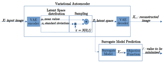
Figure 1.
Main elements of the DL model.
2.1. Variational Autoencoder
An autoencoder (AE) is a type of artificial neural network belonging to the unsupervised learning category [1]. AEs can be used to learn the efficient encoding of the input high-dimensional patterns, representing them in a lower dimensional space (latent space). The performance of the encoding is validated and refined by attempting to regenerate the input from its representation in the latent space. The autoencoder is typically used for dimensionality reduction, by training the network to ignore irrelevant data.
A VAE is an autoencoder whose encoding is regularized during the training in order to ensure that its latent space has good properties allowing the generation of new data. Instead of encoding an input as a single point, a VAE encodes it as a distribution (a mean value and standard deviation) over the latent space. First, the input is encoded as distribution over the latent space; second, a point from the latent space is sampled from that distribution using the so-called reparameterization trick; third, the sampled point is decoded to form the reconstructed pattern. The reason for which an input is encoded as a distribution with some variance instead of a single point is that it makes enables the very natural expression of latent space regularization: the distributions returned by the encoder are enforced to be close to a standard normal distribution. Thus, the loss function that is minimized when training a VAE is composed of a “reconstruction term”, that tends to enhance the encoding–decoding scheme’s performance as much as possible, and a “regularization term”, that tends to regularize the organization of the latent space by making the distributions returned by the encoder close to a standard normal distribution. This regularization term is expressed as the Kulback–Leibler divergence [17] between the returned distribution and a standard Gaussian.
Autoencoder Regularization
The main aspects of a VAE are depicted in Figure 1. Given an input image , the encoder neural network generates two dimensional vectors as output, where is the dimension of the latent space. In particular, the encoder is a neural network that generates the vector of mean values and the corresponding standard deviations , representing the latent distribution associated with the input:
The reparameterization trick consists of sampling a random vector from the distribution:
where . The sampled point is then used as the input of the decoder neural network, which aims to reconstruct the input image:
The loss in VAEs, also called the evidence lower bound () loss, is defined as a sum of two separate loss terms:
The first term is the reconstruction loss that measures how close the decoder output is to the original input by using the mean-squared error:
The Kullback-Leibler divergence, or KL loss, measures the difference between two probability distributions. Minimizing the KL loss in this case means ensuring that the learned means and variances are as close as possible to those of the normal distribution. For a latent dimension of size , the KL loss is obtained as
where and are, respectively, the k-th element of vectors and obtained using the encoder (1).
As a consequence of the trade-off between the reconstruction error and the Kullback–Leibler divergence, the latent space of a variational autoencoder is, in general, smooth and well behaved with respect to the latent space of a standard autoencoder that minimizes the sole reconstruction error.
2.2. Surrogate Model for Optimization in the Encoded Latent Space
The surrogate model is a neural network that accepts a pattern (obtained from a bitmap using Equations (1) and (2)) belonging to the latent space as input and predicts the output physical variables (i.e., induction filed values at desired points in space):
The loss function of the SM training is the mean square error:
where represents the ground truth target values of the physical variables corresponding to the input geometry (induction field pattern corresponding to input image obtained from FEA simulations as described in Section 3.4).
Objective Function
In the proposed framework, the objective function to be minimized defines a scalar physical quantity f which is a known analytical function of the physical variables , as predicted by the surrogate model:
As an alternative, if an analytical expression of the objective function is not available, it can be defined as a direct output of the surrogate model:
In the latter case, evidently, the intermediate prediction of is not needed.
2.3. Multi-Model Custom Training Loop
In order to train the VAE and the SM, we define a custom training loop where the learnable parameters of both models are updated by means of the gradient of a global loss function, which is a combination of the loss functions of the two models:
where the weights and are empirically determined so that the three terms have roughly the same order of magnitude. Figure 2 shows the corresponding flux diagram. The gradient of the total loss E with respect to the learnable parameters of the models is calculated using automatic differentiation [25]. The parameters can then be updated using the gradient descent rule, or using more advanced update rules such as adaptive moment estimation (Adam) [26].
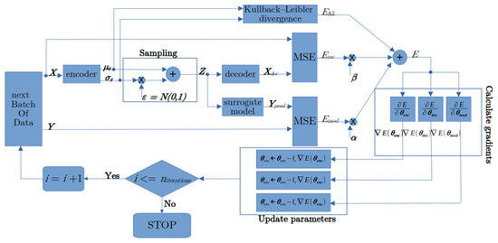
Figure 2.
Flux diagram of the custom training loop.
The complete pseudocode of the custom training loop is reported in Algorithm 1. In particular, Algorithm 1 is a custom neural network training algorithm which has the scope to train three neural networks at the same time: the and of the VAE, and the , which are described by their learnable parameters, respectively, , and . Consequently, the input of the training algorithm is the training set, represented by the input and target datasets , which are shown at the top of Algorithm 1 (pseudo-code lines 1 and 2), and the output is represented by the trained learnable parameters , and , which are shown at the bottom of Algorithm 1 (pseudo-code lines 28, 29 and 30). The learnable parameters include weights and biases. The weights were initialized using Glorot [27] initialization, while the biases were initialized with zero. The generation of the training dataset will be described in detail in the following sections.
| Algorithm 1 Multi-Model Custom Training Loop Pseudocode. | |
| 1: input training dataset of geometry images | ▹ matrix of size |
| 2: target training dataset of magnetic field values | ▹ matrix of size |
| 3: | ▹ initialization |
| 4: | |
| 5: | ▹ batch size |
| 6: | ▹ learning rate for stochastic gradient optimization |
| 7: | |
| 8: randomly initialize learnable parameters | |
| 9: randomly initialize learnable parameters | |
| 10: randomly initialize learnable parameters | |
| 11: empirical value | |
| 12: empirical value | |
| 13: for do | ▹ custom training loop |
| 14: | ▹ matrix of size |
| 15: | ▹ matrix of size |
| ▹ returns non overlapping subset of consecutive points from | |
| 16: | ▹ Apply variational encoder, |
| ▹ and are matrices of size | |
| 17: | ▹ pick a random scalar point from normal distribution |
| 18: | ▹ sampling: reparameterization trick |
| ▹ is a matrix of size | |
| 19: | ▹ decoded image: matrix of size |
| 20: | ▹ predicted output: matrix of size |
| 21: | ▹ Kullback–Leibler divergence |
| 22: | ▹ reconstruction loss |
| 23: | ▹ surrogate model loss |
| 24: | ▹ total loss |
| 25: | ▹ total loss gradient wrt parameters |
| 26: | ▹ total loss gradient wrt parameters |
| 27: | ▹ total loss gradient wrt parameters |
| ▹ note: gradients are calculated by means of automatic differentiation | |
| 28: | ▹ update paramenters |
| 29: | ▹ update paramenters |
| 30: | ▹ update paramenters |
|
▹ note: here vanilla stochastic gradient descent approach is reported, more advanced update algorithms may be used such as Adam | |
| 31: end for | |
Regarding the complexity of the algorithm, we can state that in our case the known results regarding the computational complexity of the backpropagation algorithm apply directly [28]. In fact, we use backpropagation to train the three models in order to minimize the same loss function E, which is a combination of the three loss functions of the separate models (11).
It is worth noting that the simultaneous training of the VAE and SM has a deep semantic impact with respect to training the models separately. In particular, the encoder affects all three losses and . As a consequence, the encoder will also be trained to minimize the loss that would otherwise only be a function of the surrogate model. On the other hand, the SM was trained using a latent space that is in gradual definition during the simultaneous VAE training, forcing the encoder to adapt the latent representation to the desired features of the SM, and allowing, at the same time, to regularize the training of the SM and preventing the SM from overfitting. This procedure can result in a worse value of the reconstruction loss, but with the benefit of a better global performance.
2.4. Optimization Loop
Algorithm 2 is an optimization algorithm which has the scope of minimizing the objective function introduced in Equation (9), and is further defined for its particular application in Equation (13) of the following section. For this reason, the input of the algorithm is represented by the full definition of the objective function, which is given by Equations (9) and (13), and by the neural networks described in Equations (1), (2) and (7). The output of the model is the design geometry for which we have the optimal value. The optimization was completely carried out in the latent space, using only the neural models (there is no finite element analysis in the loop), and the optimal geometry is obtained by decoding the final solution. Algorithm 2 shows the pseudocode of the optimization loop, while Figure 3 shows the corresponding flux-diagram. We use a starting geometry as an initial guess, which is encoded to (as an alternative, a random can be used as well).Successively, a classic gradient descent optimization is performed, evaluating the surrogate model and the corresponding objective function is reached until a maximum number of iterations (or until another stop criterion is triggered).
| Algorithm 2 Optimization Loop Pseudocode. | |
| 1: | ▹ step size of gradient descent optimization |
| 2: | ▹ desired induction field at control points |
| ▹ is a matrix of size | |
| 3: initial geometry | ▹ matrix of size |
| 4: | ▹ Apply variational encoder, |
| 5: | ▹ pick a random scalar point from normal distribution |
| 6: | ▹ sampling: reparameterization trick |
| ▹ matrix of size | |
| 7: | |
| 8: for do | ▹ optimization loop |
| 9: | ▹ predicted output: matrix of size |
| 10: | ▹ calculate TEAM 25 objective function (13) |
| 11: | ▹ calculate gradient of f wrt |
| 12: if then | |
| 13: break for | ▹ terminate if gradient below tolerance |
| 14: end if | |
| 15: | ▹ gradient descent update rule |
| 16: end for | |
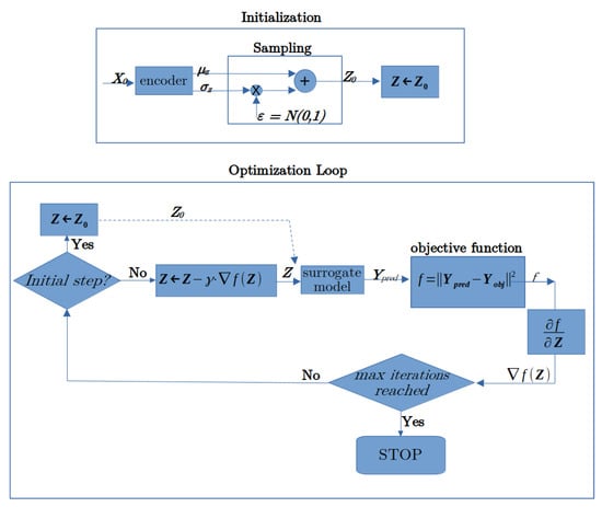
Figure 3.
Flux diagram of the optimization loop.
The quantity to optimize f is algorithmically calculated as a function of , therefore, automatic differentiation can be used to conveniently determine the gradient of f with respect to . In our experiments, optimal values of f were obtained with a relatively small number (below 100) of gradient descent update steps corresponding to the pseudocode in Algorithm 2 line 15. In our test case, the objective function is analytically defined as a function of the induction fields calculated by the surrogate model, but it is worth noting that an analytical definition of the objective function is not necessarily required. In fact, as mentioned previously, thanks to automatic differentiation, the proposed approach can also be used in the case that the objective function is directly predicted by the surrogate model.
As a final comment, each value of obtained during the gradient descent search can be decoded to the corresponding geometry, and the evolution of the geometry during optimization can be visualized, observing how undesired features gradually disappear, while desired ones appear.
Regarding the complexity (intended as the time cost as a function of the number of variables) of the optimization algorithm, it generally depends on the complexity of the function to be optimized. In our case, we can say that, for a fixed objective function, the complexity of the algorithm is linear with respect to the number of iterations .
3. Selected Test Case: TEAM 25 Problem
In order to test the approach, we applied it to the TEAM 25 problem [29]. Testing electromagnetic analysis methods (TEAM ) is a series of benchmark problems used in the area of computational electromagnetics, and represents an open international working group aiming to compare electromagnetic analysis computer codes. In particular, TEAM 25 aims to compare the performance of different topology optimization algorithms on a design problem for an electromagnetic die press. The geometry that describes the problem [29] is shown in Figure 4. The objective is to design the two die molds in order to achieve a radial induction field, with a constant magnitude in nine control points, , uniformly placed along the arc of circumference inside the cavity between the molds. In particular, the target induction field along the line according to the TEAM 25 problem definition is:
where is the azimuthal coordinate of the target point for . The nine points were placed so that the radius is constant and equal to and the azimuthal coordinates are distributed as . The objective was to design the shape of the die molds so that the following error function is minimized:
where is the field obtained in the target point for a given design. In particular, introducing the following vector notation:
Equation (13) can be rewritten as
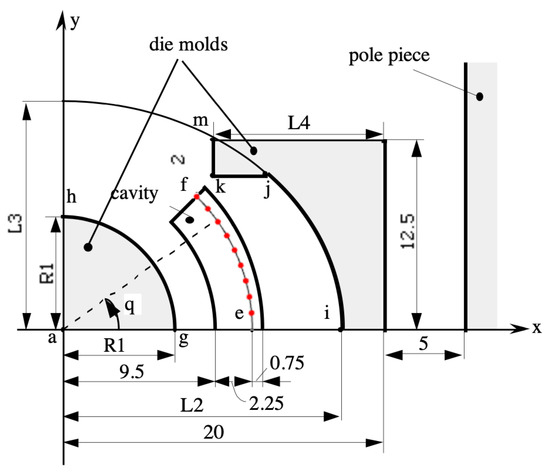
Figure 4.
Geometry of the mold for the TEAM 25 problem—measures are in mm.
In this paper, we address the so-called large ampere turns case (17,500 AT), for which the problem definition specifies that the curve (the right mold) can be considered a “free curve”. This choice allows us to exploit the full potential of the topology optimization proposed approach, where the bitmap representation describes the free geometry with flexibility. In contrast, most of the works in the literature addressed the small AT case, which defines a simpler geometry parametrization that can be solved easier with standard optimization approaches.
3.1. FEA Model
An accurate finite element model of the TEAM 25 problem was developed using the commercial software Comsol [30]. Considering the magnetostatic nature of the problem, and the lack of sources in the region of study, the formulation implemented in the software exploits symmetry and is based on the magnetic scalar potential. This choice let us reduce the spatial domain to the one enclosed by the pole pieces, without the need for considering the electromagnet. The value of the magnetic scalar potential difference (between the two poles) was straightforwardly obtained from the values of the ampere-turns excitation. In addition, symmetry can be exploited, further reducing the domain to of the space between the poles. The problem description also specifies the ferromagnetic material characteristic (), given as a set of sampling points that were implemented in the software. The symmetry plane and the remaining border of the domain were defined as magnetics insulation borders, the latter located at the proper distance. A fine mesh was adopted, in order to take into account the discrete nature of the right mold surface, averagely resulting in approximately 5000 domains and 300 boundary elements.
Figure 4 shows the main aspects of the geometry of the implemented model, with the left mold ( curve) being an arc of circumference characterized by the radius parameter , the right mold ( curve) being implemented as a free shape, and the nine red control points along the curve being used to define the objective function (13).
3.2. Full FEA-Based Optimization and Model Validation
As a term of comparison, we report the result of a previous work [7], where we performed a full FEA-based optimization of the geometry. Within this frame of reference, the right mold was implemented as a piecewise-constant profile with steps of 5 mm in the y direction, in order to allow a geometry representation that is similar to the bitmap representation that will be used in the following approaches based on deep learning. The optimization was performed using the Comsol optimization module, particularly the bound optimization by quadratic approximation method (BOQAM). The stopping criterion was based on the so-called “optimality tolerance”, i.e., the search was stopped as soon as no improvement over the current best estimate can be found larger than (or equal to) the optimality tolerance parameter. The time required by one simulation with FEA was 3 s in an Intel I7 computer with 6 cores and 12 threads. Several optimization runs were performed, and similar results were obtained, both in terms of optimal objective function value and corresponding geometry. On average, a single optimization run terminates after 2000 function evaluations, thus requiring a total average time of 6000 s. Figure 5 shows the final geometry resulting from one optimization run. In this case, the left mold radius was also optimized. The objective function value of the this optimal solution was , which is comparable to the known solutions from the literature [31].
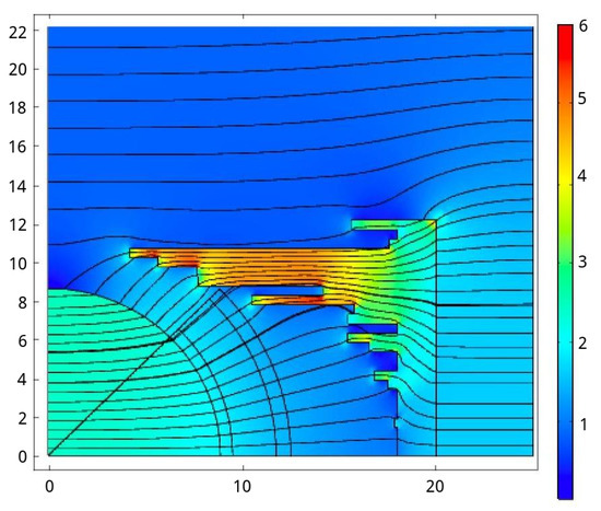
Figure 5.
Optimal design using a commercial software— parameter is also optimized.
Regarding the sensitivity analysis, the optimization showed that, in order to reach very low values of the error function, the value of the parameter (the radius of the curve which is the arc of circumference describing the left mold) tends to be close to the maximum allowed value (13). The optimization of the left mold is then trivial. For this reason, and to better analyze and compare the proposed deep learning approach with respect to full FEA-based optimization, it was decided to consider the value of the to be constant and equal to an intermediate value of 5 mm, providing to the optimization procedure the ability to exclusively operate on the free curve of the right mold. With this stance, the resulting optimal values cannot reach such small values as in the case of the optimized left mold radius , defining a difficult topology optimization problem that has not yet been addressed in the literature, but which is a well-posed problem to be approached with advanced optimization procedures. The results of the optimization with fixed using both the Comsol optimization module and the proposed deep learning approach will be shown in Section 5.
3.3. Bitmap Representation of Geometry
In the subsequent part of the paper, the geometry of the problem will be represented using a bitmap approach. In particular, using a profile discretization of 0.5 mm along both the x and y directions, the topological space can be represented by a binary bitmap with a resolution of (900 pixels), where only the right mold, i.e., the free curve in Figure 4, is of interest. Figure 6 shows the topology of the bitmap representation, where the right mold occupation was maximized, filling all the possible pixels that do not overlap with the cavity, which represents our main geometrical constraint. In particular we represent with a black square (pixel = 1) a portion of space filled with ferromagnetic material, while a white square (pixel = 0) represents an empty portion of space. Considering Figure 6, all feasible solutions can be obtained by removing one or more black pixels, while an empty space cannot be filled without violating the constraints.
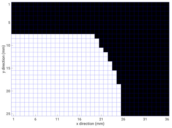
Figure 6.
Bitmap representation of the topological space. We represent with a black square (pixel = 1) a portion of space filled with ferromagnetic material, while a white square (pixel = 0) represents an empty portion of space. In this figure, the right mold occupation is maximized.
3.4. Dataset Generation
To allow the training of the neural models, a number of 10,000 bitmaps of the right mold were generated using the above-described representation, thus fulfilling the problem constraints.
In order to obtain physically reasonable geometries, the following additional constraints were imposed over the random generation:
- The ferromagnetic material is characterized by a connected shape with no holes,
- The probability of empty cells decreases along the positive y direction.
The second condition was imposed to increase the probability of generating geometries that follow the shape of the cavity.
An FEA simulation was carried out using Comsol for each generated profile, obtaining the corresponding and field distribution in the nine target points. The dataset for deep learning then consists of the 10,000 input images of dimension and the corresponding 10,000 induction field patterns of dimension , which represents the output. In the following, we use to denote input images, while stands for the output induction field patterns.
4. Selection of Model Architecture and Testing
Once trained, the combination of the VAE with the SM forms a deep-learning surrogate model that we denote as the VAE + SM model, which predicts the field distribution with a profile image as input. Using the generated dataset of 10,000 images of geometries and the corresponding induction fields, a model selection procedure was carried out to design the architecture of the neural networks constituting the encoder, the decoder and the surrogate model.
It is important to note that in the community of deep learning, the use of cross-validation to determine the hyper-parameters is not a common practice as in the community of machine learning (ML), as it requires a very high computational effort in the presence of very large datasets and complex networks. In our case, the size of the dataset and the number of variables is somewhat on the edge between typical ML and DL applications. This allows us to adopt cross-validation to determine some parameters, such as the dimensionality of the VAE latent space. Regarding other parameters of the CNNs, we used the common approach of the DL community, which is mainly empirical. In fact, “optimizing hyperparameters in Convolutional Neural Network (CNN) is a tedious problem for many researchers and practitioners. To get hyperparameters with better performance, experts are required to configure a set of hyperparameter choices manually. The best results of this manual configuration are thereafter modeled and implemented in CNN” [32].
4.1. Autoencoder Architecture
The architectures of the encoder and decoder utilized in this paper are shown in Table 2 and Table 3, respectively. In particular, the encoder has an input layer that accepts images of size , two convolutional layers, two rectified linear unit (relu) layers and a fully connected output layer of size . No max pooling layers are inserted, as the image reduction is obtained by means of stride equal to 2 in the convolutional layers. The decoder has an input layer that accept patterns of dimension , and four transposed convolutional layers that upscale the latent space back to the dimension of the input space. The encoder and decoder layers’ architectures were designed using an empirical approach and previous knowledge of DL models, while the dimension of the latent space was determined using 5-fold cross-validation on the reconstruction error, resulting in an optimal value of . We were very careful to avoid test set leakage: we performed a 5-fold cross-validation using 8000 training samples only, where each fold contained 1600 points (2000 points of the test set were not used during the model selection phase).
Table 2.
Encoder architecture.
Table 3.
Decoder architecture.
In our previous work [7], we compared the nonlinear dimensionality reduction given by standard AE with the linear PCA approach, and we found that both methods indicated the same number of reduced features equal to 10. The VAE used in this work indicates a greater value of the latent space dimension equal to 25. As a general behavior, the VAEs tend to generate a latent space with increased dimensionality with respect to AEs and other feature reduction techniques, due to the regularization approach [1]. Nonetheless, the increased dimensionality of the latent space is not critical in our case, because the surrogate model and the optimization can work perfectly with 25 features. In fact, the new model outperforms the previous one, even if it works with more variables. This can be explained by the fact that the latent space was optimized, taking into account the surrogate model and the regularization term, producing a search space that is well conditioned for optimization.
4.2. Surrogate Model Architecture
The architecture of the SM is reported in Table 4, and consists of a one hidden layer feed-forward neural network. The size of the hidden layer was determined using cross validation.
Table 4.
Surrogate model architecture.
4.3. Testing of the VAE + SM Model
In order to test the accuracy of the trained model, we used 8000 images to train the model and the remaining 2000 images to test the generalization capability of the model.
4.3.1. Test Errors
Given a particular input image, we calculated the normalized root mean square error of the corresponding output pattern as
The average over all the points of the test set was . This result shows that the model can predict the induction field corresponding to a given image profile with good accuracy of , which improves the accuracy of obtained in a previous work using a standard autoencoder [7], and where the SM was trained separately.
4.3.2. Regularization Considerations
The trends of the error of the VAE and the surrogate model on the test dataset during training are shown in Figure 7. It is important to note that the trend of the test error of the surrogate model is monotonically non-increasing, thus not showing evidence of overfitting. In fact, in the case of overfitting, the model learns to perfectly predict the training data, but gradually loses accuracy on test data, penalizing the capability of the generalization of the neural network. In our custom training procedure, we do not use classic techniques to directly prevent the overfitting of the surrogate model neural network (such as Bayesian regularization or using a validation set), as the regularization is implicitly imposed by minimizing the combined loss funcion (11) on the training dataset.
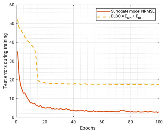
Figure 7.
Trend of the test errors during training. No overfitting can be observed, thanks to implicit regularization.
4.3.3. Reconstruction Capability
The ability of the decoder to reconstruct the original input image is shown in Figure 8, whereas Figure 9 depicts some randomly generated profiles using the VAE as a generative model, where we randomly sampled values of from a normal distribution to feed the decoder. It is worth noting that the trained VAE perfectly learned the constraints of the geometry from the training data: in all our simulations, the output of the decoder always generated feasible geometries, even in the case of being used as a generative model.
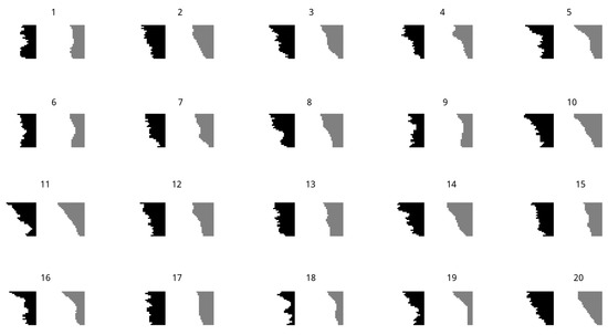
Figure 8.
Some input geometries (in black on the left side) and the corresponding VAE reconstruction (in gray on the right side).
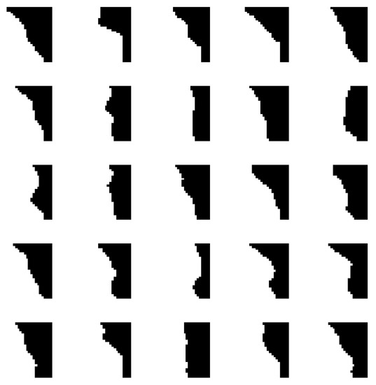
Figure 9.
Some VAE randomly generated geometries.
4.4. Latent Space Visualization
Elucidating the good properties of the latent space of the VAE was principal motivation of this work, and in this section, we aim to evidence how the data are distributed in the latent space with respect to the corresponding values of the objective function f, which is defined in Equation (13). For this reason, we performed the principal component analysis (PCA) of the latent space data, particularly of the distribution of 10,000 vectors corresponding to each input image. A scatter plot of the first three principal components (PCs) can be visualized in Figure 10, where the color of the markers is proportional to the f value of the corresponding geometry. It can be observed that a gradual and coherent transition of f values from high to low is present in the distribution. Optimal points are concentrated in a particular region (bright yellow colors), and a gradient descent approach is expected to perform well in such a search space, where the optimal region is convex and there are no other evident local minima.
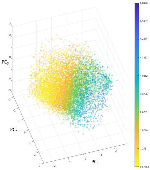
Figure 10.
PCA analysis of the latent space of the VAE. Each point corresponds to a geometry belonging to the generated dataset and the color of the markers is proportional to the corresponding f value (13).
5. Results and Discussion
The optimal profile obtained by the optimization using the proposed approach is shown in Figure 11, which also shows a comparison with the results of the commercial software (full FEA approach) mentioned in Section 3.1 in the case of fixed = 5 mm, and with the optimal result that was obtained in a previous work [7]. The value of the objective function is for the solution obtained with the proposed VAE + SM method, which improves both the value obtained with the full FEA optimization, , and the result obtained in the previous work [7], . In particular, in [7], the AE and the surrogate model were trained separately, and the optimization was carried out with a GA.
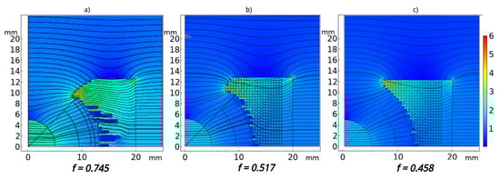
Figure 11.
Optimal geometries and flux density norm. Cases (a–c) correspond, respectively, to the full FEA-based optimization, the previous work [7] and the proposed solution in this work.
The evolution of the geometry during optimization was visualized, observing how undesired features gradually disappear while desired ones appear, in Figure 12, where an initial bad solution gradually transforms into a good solution. The final solution results to be practically independent from the starting point, which is a consequence of the absence of local minima.
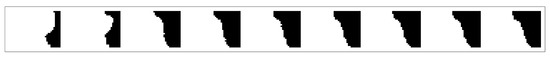
Figure 12.
Evolution of decoded geometries during optimization, showing one frame every 10 optimization steps.
The time cost of the VAE + SM optimization approach, excluding the generation of the training set, is two orders of magnitude lower that of the full FEA-based optimization, allowing much better domain exploration: dozens of (<100) function and gradient evaluations need to be performed instead of a few hundred (1740) performed by the full FEA-based optimization. In Table 5, a comparison of the methods is reported for the sole optimization phase, considering the time cost for optimization and the number of function evaluations obtained as average values over multiple runs. The VAE + SM training-related costs are shown in Table 6. The total time cost of the VAE + SM approach results as very similar to the time cost of the previous approach using a standard autoencoder and separate training [7]—even if the VAE used in this work is a much complex model than the AE used in [7]. All of the simulations of this work and previous works [7] were carried out on the same machine: a PC with a 6-core Intel I7 5820 k processor and 32 GB of RAM.
Table 5.
Average optimization performance over 50 runs and comparison with other metods.
Table 6.
Model training-related costs.
In the interest of completeness, regarding the training phase, we used similar—but not identical—stop criteria with respect to the previous work. In [7], the training of the autoencoder was stopped after 80 epochs “as gradient values were below the tolerance of ”, whereas in this work, the training of the VAE + SM was stopped after 100 epochs, because no further improvement over the test errors were observed (Figure 7). In the new model proposed in this paper, it is not trivial to define a criterion based on the values of the gradient because the multi-model training simultaneously uses three gradients, as can be observed in Algorithm 1. In any case, the time for training the VAE + SM for 100 epochs using Algorithm 1 was very similar to the time for training the AE and the SM separately.
We can summarize the advantages and disadvantages of the proposed approach as follows.
Advantages of the proposed approach
- The latent space of the VAE is more regular than the latent space of a standard AE. This regularity facilitates the search for the optimal solutions;
- The gradient descent algorithm requires a much lower computational cost with respect to the evolutionary optimization algorithms—it can reach the optimum with dozens of function evaluations instead of tens of thousands;
- If the training dataset represents a large distribution of behaviors, it can be used to formulate and solve a number of different problems with very low computational time;
- Simultaneous (parallel) training of a complex VAE + SM model requires a computational time comparable to separate (series) training of a simpler AE + SM model [7];
- The proposed approach provides very useful insight and visualization of the optimization process, which is not possible using evolutionary optimization algorithms such as GAs.
Disadvantages with respect to other approaches
- The training dataset needs to be carefully designed and created, which it is a difficult and time-consuming task, requiring expert knowledge in terms of the application;
- In the case of a very irregular search space, the gradient descent algorithm could be trapped in local minima, thus requiring the use of global optimization methods such as Adam.
6. Conclusions
Pursuing research for the most effective use of machine learning in the area of computational electromagnetics, in this paper, we analyzed the impact of combined learning for the autoencoder and surrogate model on the performance of a DL model to be used in the topology optimization of electromagnetic devices. As a matter of fact, a bit-wise representation of the geometrical characteristics for the domain whose topology is to be optimized allows the discovery of new designs, hardly reachable when using parametrized representation. On the other hand, unparametrized design requires considerable computational resources in the electromagnetic analysis phase, and the advent of machine learning to generate surrogate models guaranteeing satisfactory performance also allowed testing such approaches on desktop-class computers. Finally, the adoption of regularized procedures, proposed in this paper, allows avoiding unfeasible geometries, but also using derivative-based optimization algorithms. It is important to point out that the training dataset strongly affects the performance of the optimization, because it defines the manifold where the optimal solution is searched. One benefit is that the constraints are automatically fulfilled, whereas a drawback is that the search will be confined inside this manifold. Therefore, the training set shall be generated in order to well represent the topological space, including promising regions where the optimal solution is expected to be found. In this paper, a VAE using CNNs was tested for the creation of a DL model to be used for the resolution of the TEAM 25 test problem. The approach proved to be capable of improving the quality of optimized topology, within the time of one order of magnitude lower than the classical topology optimization (once training of the DL model is achieved).
One of the open problems of topology optimization is related to the practical realizability of the obtained optimal designs: the optimal geometry obtained as a bitmap in some cases needs to be smoothed and modified to fulfill the requirements and constraints of the industrial process for production. In terms of future work, these constraints may be included in the optimization or in the dataset generation in order to obtain final designs that are close to the realizable shapes.
The process of creating the training dataset is one of the trickiest parts of the proposed approach, as it requires human interaction and empirical knowledge of application. As future work, the dataset generation could be partially automated, for example, exploiting the data gathered during the optimization process of a full FEA approach. In fact, during the search process, a full FEA optimization generates input–output patterns that could be used to populate the training dataset, with the advantage of generally representing nearly optimal solutions—which is accidentally a desired feature of the training dataset.
Author Contributions
Conceptualization, all authors; methodology, M.T.; software, M.T.; validation, M.T., D.T.; formal analysis, A.F., S.B.; data curation, D.T., M.T.; writing—original draft preparation, M.T.; writing—review and editing, A.F., S.B., M.T.; visualization, D.T.; supervision, A.F., S.B. All authors have read and agreed to the published version of the manuscript.
Funding
This research received no external funding.
Conflicts of Interest
The authors declare no conflict of interest.
Abbreviations
The following abbreviations are used in this manuscript:
| DL | Deep Learning |
| ML | Machine Learning |
| CNN | Convolutional Neural Networks |
| TEAM | Testing Electromagnetic Analysis Methods |
| AE | Autoencoder |
| VAE | Variational Autoencoder |
| GA | Genetic Algorithm |
| PSO | Particle Swarm Optimization |
| SM | Surrogate Model |
| FEA | Finite Element Analysis |
| MSE | Mean Square Error |
| ELBO | Evidence Lower Bound |
| KL | Kullback–Leibler |
| Adam | Adaptive Momentum Estimation |
| FEM | Finite Element Model |
| AT | Ampere Turns |
| BOQAM | Bound Optimization by Quadratic Approximation Method |
| PCA | Principal Component Analysis |
| PC | Principal Component |
| relu | Rectified Linear Unit |
| NRMSE | Normalized Root Mean Square Error |
| EM | Electromagnetic |
References
- Goodfellow, I.; Bengio, Y.; Courville, A. Deep Learning; MIT Press: Cambridge, UK, 2016. [Google Scholar]
- Alom, M.Z.; Taha, T.M.; Yakopcic, C.; Westberg, S.; Sidike, P.; Nasrin, M.S.; Asari, V.K. A state-of-the-art survey on deep learning theory and architectures. Electronics 2019, 8, 292. [Google Scholar] [CrossRef] [Green Version]
- Zhang, P.; Hu, Y.; Jin, Y.; Deng, S.; Wu, X.; Chen, J. A Maxwell’s Equations Based Deep Learning Method for Time Domain Electromagnetic Simulations. IEEE J. Multiscale Multiphys. Comput. Tech. 2021, 6, 35–40. [Google Scholar] [CrossRef]
- Li, Y.; Lei, G.; Bramerdorfer, G.; Peng, S.; Sun, X.; Zhu, J. Machine Learning for Design Optimization of Electromagnetic Devices: Recent Developments and Future Directions. Appl. Sci. 2021, 11, 1627. [Google Scholar] [CrossRef]
- Gabdullin, N.; Madanzadeh, S.; Vilkin, A. Towards End-to-End Deep Learning Performance Analysis of Electric Motors. Actuators 2021, 10, 28. [Google Scholar] [CrossRef]
- Parekh, V.; Flore, D.; Schöps, S. Deep Learning-Based Prediction of Key Performance Indicators for Electrical Machines. IEEE Access 2021, 9, 21786–21797. [Google Scholar] [CrossRef]
- Barmada, S.; Fontana, N.; Formisano, A.; Thomopulos, D.; Tucci, M. A Deep Learning Surrogate Model for Topology Optimization. IEEE Trans. Magn. 2021, 57, 1–4. [Google Scholar] [CrossRef]
- Brescia, E.; Costantino, D.; Massenio, P.R.; Monopoli, V.G.; Cupertino, F.; Cascella, G.L. A Design Method for the Cogging Torque Minimization of Permanent Magnet Machines with a Segmented Stator Core Based on ANN Surrogate Models. Energies 2021, 14, 1880. [Google Scholar] [CrossRef]
- Barmada, S.; Fontana, N.; Sani, L.; Thomopulos, D.; Tucci, M. Deep Learning and Reduced Models for Fast Optimization in Electromagnetics. IEEE Trans. Magn. 2020, 56, 1–4. [Google Scholar] [CrossRef]
- Barmada, S.; Fontana, N.; Thomopulos, D.; Tucci, M. Autoencoder Based Optimization for Electromagnetics Problems. ACES J. 2019, 34, 1875–1880. [Google Scholar]
- Sasaki, H.; Igarashi, H. Topology Optimization Accelerated by Deep Learning. IEEE Trans. Magn. 2019, 55, 1–5. [Google Scholar] [CrossRef] [Green Version]
- Doi, S.; Sasaki, H.; Igarashi, H. Multi-Objective Topology Optimization of Rotating Machines Using Deep Learning. IEEE Trans. Magn. 2019, 55. [Google Scholar] [CrossRef]
- Asanuma, J.; Doi, S.; Igarashi, H. Transfer Learning Through Deep Learning: Application to Topology Optimization of Electric Motor. IEEE Trans. Magn. 2020, 56. [Google Scholar] [CrossRef]
- Khan, A.; Ghorbanian, V.; Lowther, D. Deep Learning for Magnetic Field Estimation. IEEE Trans. Magn. 2019, 55. [Google Scholar] [CrossRef]
- Khan, A.; Mohammadi, M.H.; Ghorbanian, V.; Lowther, D. Efficiency Map Prediction of Motor Drives Using Deep Learning. IEEE Trans. Magn. 2020, 56. [Google Scholar] [CrossRef]
- Kingma, D.P.; Welling, M. Auto-encoding variational bayes. arXiv 2013, arXiv:1312.6114. [Google Scholar]
- Kingma, D.P.; Welling, M. An introduction to variational autoencoders. arXiv 2019, arXiv:1906.02691. [Google Scholar] [CrossRef]
- Yang, Y.; Zheng, K.; Wu, C.; Yang, Y. Improving the classification effectiveness of intrusion detection by using improved conditional variational autoencoder and deep neural network. Sensors 2019, 19, 2528. [Google Scholar] [CrossRef] [Green Version]
- Lopez-Martin, M.; Carro, B.; Sanchez-Esguevillas, A.; Lloret, J. Conditional variational autoencoder for prediction and feature recovery applied to intrusion detection in iot. Sensors 2017, 17, 1967. [Google Scholar] [CrossRef] [Green Version]
- Vo, T.H.; Lee, G.S.; Yang, H.J.; Oh, I.J.; Kim, S.H.; Kang, S.R. Survival Prediction of Lung Cancer Using Small-Size Clinical Data with a Multiple Task Variational Autoencoder. Electronics 2021, 10, 1396. [Google Scholar] [CrossRef]
- Goodfellow, I.J.; Pouget-Abadie, J.; Mirza, M.; Xu, B.; Warde-Farley, D.; Ozair, S.; Bengio, Y. Generative adversarial networks. arXiv 2014, arXiv:1406.2661. [Google Scholar] [CrossRef]
- Tripp, A.; Daxberger, E.; Hernández-Lobato, J.M. Sample-efficient optimization in the latent space of deep generative models via weighted retraining. Adv. Neural Inf. Process. Syst. 2020, 33, 1–14. [Google Scholar]
- Winter, R.; Montanari, F.; Steffen, A.; Briem, H.; Noé, F.; Clevert, D.A. Efficient multi-objective molecular optimization in a continuous latent space. Chem. Sci. 2019, 10, 8016–8024. [Google Scholar] [CrossRef]
- Oh, S.; Jung, Y.; Kim, S.; Lee, I.; Kang, N. Deep generative design: Integration of topology optimization and generative models. J. Mech. Des. 2019, 141, 111405. [Google Scholar] [CrossRef] [Green Version]
- Baydin, A.G.; Pearlmutter, B.A.; Radul, A.A.; Siskind, J.M. Automatic Differentiation in Machine Learning: A Survey. J. Mach. Learn. Res. 2018, 18, 1–43. [Google Scholar]
- Kingma, D.P.; Ba, J. Adam: A method for stochastic optimization. arXiv 2014, arXiv:1412.6980. [Google Scholar]
- Glorot, X.; Bengio, Y. Understanding the difficulty of training deep feedforward neural networks. In Proceedings of the Thirteenth International Conference on Artificial Intelligence and Statistics, Sardinia, Italy, 13–15 May 2010; pp. 249–256. [Google Scholar]
- Livni, R.; Shalev-Shwartz, S.; Shamir, O. On the computational efficiency of training neural networks. arXiv 2014, arXiv:1410.1141. [Google Scholar]
- Takahashi, N.; Ebihara, K.; Yoshida, K.; Nakata, T.; Ohashi, K.; Miyata, K. Investigation of simulated annealing method and its application to optimal design of die mold for orientation of magnetic powder. IEEE Trans. Magn. 1996, 32, 1210–1213. [Google Scholar] [CrossRef]
- COMSOL-Software for Multiphysics Simulation. Available online: www.comsol.com (accessed on 13 July 2020).
- Carcangiu, S.; Fanni, A.; Mereu, A.; Montisci, A. Grid-Enabled Tabu Search for Electromagnetic Optimization Problems. IEEE Trans. Magn. 2010, 46, 3265–3268. [Google Scholar] [CrossRef]
- Aszemi, N.M.; Dominic, P.D.D. Hyperparameter optimization in convolutional neural network using genetic algorithms. Int. J. Adv. Comput. Sci. Appl. 2019, 10, 269–278. [Google Scholar] [CrossRef]
Publisher’s Note: MDPI stays neutral with regard to jurisdictional claims in published maps and institutional affiliations. |
© 2021 by the authors. Licensee MDPI, Basel, Switzerland. This article is an open access article distributed under the terms and conditions of the Creative Commons Attribution (CC BY) license (https://creativecommons.org/licenses/by/4.0/).