A New 4D Hyperchaotic System and Its Analog and Digital Implementation

Abstract

This work presents a new four-dimensional autonomous hyperchaotic system based on Méndez-Arellano-Cruz-Martínez (MACM) 3D chaotic system. Analytical and numerical studies of the dynamic properties are conducted for the new hyperchaotic system (NHS) in its continuous version (CV), where the Lyapunov exponents are calculated. The CV of the NHS is simulated and implemented using operational amplifiers (OAs), whereas the Discretized Version (DV) is simulated and implemented in real-time. Besides, a novel study of the algorithm performance of the proposed DV of NHS is conducted with the digital-electronic implementation of the floating-point versus Q1.15 fixed-point format by using the Digital Signal Processor (DSP) engine of a 16-bit dsPIC microcontroller and two external dual digital to analog converters (DACs) in an embedded system (ES).

1. Introduction

In recent years, the potential applications of chaotic systems have attracted attention as an interesting nonlinear phenomenon, since the chaotic properties are highly desired in several areas of science and engineering such as high sensitivity to initial conditions, high entropy, topology complexity, ergodicity [1,2,3], among others. These properties have an important theoretical value for the academic community and research groups about the study and design of systems that generate chaotic behavior, and they have become a crucial point for engineers with different applications in areas such as biology [4], secure communications [5], chaotic trajectories for autonomous mobile robots [6], experimental network synchronization [7], technology as fingerprint encryption [8], and digital cryptosystems based on chaos [9,10].

In 1963, Lorenz proposed a three-dimensional system with two scrolls, which is recognized as the first chaotic model reported in literature [11]. Subsequently, in 1976 Rössler proposed another chaotic system like Lorenz [12]. In 1979 Rössler proposed the first hyperchaotic system for a model of a particular chemical reaction [13]. Since then, several hyperchaotic systems have been reported, such as temperature fluctuation model [14], with memristive and electronics circuits [15,16], fractional order [17], semiconductor laser system [18], synchronization [19,20], and image encryption [21].

The mathematical definition of a hyperchaotic system is based on a chaotic system with more than one positive Lyapunov exponent, and simultaneously its dynamics are richer and more extended in the phase plane [16]. The hyperchaos has more complex dynamical behaviors than the chaotic system, and it can be found coupling k chaotic systems to obtain a hyperchaotic attractor with n positive Lyapunov exponents; the transition from chaos to hyperchaos shows that the attractor’s dimension increase and the second Lyapunov exponent grow continuously [22]. A hyperchaotic system can be numerically and experimentally generated by adding a simple state feedback controller, e.g., Chua’s circuit [23], Chen system [20], or Lorenz [24].

Recently, the electronic digital implementation of chaotic systems has attracted the attention for the community scientific for the several applications in engineering, e.g., the cryptosystems—where the main encryption process is based on chaos—are designed considering statistical and security tests, even if the cryptosystem has good performance, the computing capacity on embedded systems continues being a challenge for designers [9,10,14,17].

The computing capacity on the embedded systems such as FPGA [25,26,27], system on chip (SOC) [28], DSP [29], and 16 or 32-bit microcontrollers [26,30] continues being a challenge for designers to reproduce a chaotic system considering tools that currently have embedded systems. The algorithm of a chaotic map of discrete time can be directly implemented in an embedded system, whereas the chaotic systems of continuous time need to be discretized by using some numerical solution to be implemented in an embedded system [21]. First, we need to consider the accuracy method and the time complexity to conduct the discrete version (DV) of the chaotic system, and then we need to know the embedded system properties to implement the algorithm, where chaos degradation is unavoidable and can reduce the performance for some application. There are studies that establish techniques to avoid chaos degradation when it is implemented in embedded system [29]. The digital electronic implementation is very limited to meet the requirements as power and performance speed, memory resources, and the time complexity that algorithms based in chaos need to run many computing resources to encrypt and transfer multimedia contents such as ultra-definition video, high-fidelity audio, big-size data files [31], among others.

In this work, we firstly introduce a new 4D hyperchaotic system (NHS) via modifying 3D MACM system inspired by the above works [32]. Two critical parameters, only two nonlinearities, flexible and robust, one unstable equilibrium saddle-point, and low-cost electronic implementation for the continuous and discretized versions are the main novelties of the proposed hyperchaotic system. All these features result in a highly attracting digital implementation, such as low complexity time, high iterations per second (ips) where chaos is preserved, and it may be of great interest for engineering applications such as chaos-based cryptography, biometric systems, telemedicine, and secure communications. According to our best knowledge, the digital implementation of the nonlinear hyperchaotic dynamics in real-time of DV in Q1.15 fixed-point using the DSP engine of the dsPIC have not been reported before.

The paper is organized as follows: Section 2 reports the basic analytical proofs and the extensive numerical tests of the proposed NHS to verify the chaos and hyperchaos existence. Section 3 presents two electronic implementations to reproduce the dynamics of NHS: the first one is implemented by using OAs, the second one is implemented in ES by using dsPIC33FJ and two dual external digital-to-analog converters (DAC). In addition, a digital performance study is conducted taking into consideration the benefits of the dsPIC33FJ’s digital signal processing engine to obtain a Q1.15 fixed-point versus the floating-point versions. Finally, in Section 4 we draw some concluding remarks.

2. Basic Analysis and Characterization of New Hyperchaotic System

In this section, state equations and tests to verify the hyperchaos existence are presented. The NHS system is built by inspecting, modifying, and adding one state to the MACM chaotic system [32]. The proposed NHS is described as follows

$$\begin{array}{c}\dot{x}=-ax-byz,\\ \dot{y}=-x+cy+cw,\\ \dot{z}=d-y^2-z,\\ \dot{w}=x-w.\end{array}$$

(1)

The system (1) has ten terms, two quadratic nonlinearities, and four parameters a, b, c, d ∈ $ℝ$⁺, with c < a + 2, where b and d are characterized as the bifurcation parameters. The nonlinear NHS (1) is hyperchaotic with a = 2, b = 2, c = 0.5, and d = 14.5.

2.1. Symmetry

The system (1) is symmetrical about the z-axis for its invariance under the coordinate transformation (x, y, z, w)→(−x, −y, z, −w). The symmetry is not associated with the a, b, c, d parameters.

2.2. Dissipativity and Existence of Attractor

For a dynamical system, the divergence of 3-dimensional flow is defined by

$$\nabla V=\frac{\partial \dot{x}}{\partial x}+\frac{\partial \dot{y}}{\partial y}+\frac{\partial \dot{z}}{\partial z}+\frac{\partial \dot{w}}{\partial w}=-a+c - 1 - 1=-3.5 < 0.$$

(2)

Therefore, the above analysis proves that our system is dissipative. The exponential contraction rate is calculated as follows

$$\frac{dV}{dt}= \left(\nabla V\right)V\to {V=V}_0{e}^{-3.5t},$$

(3)

where each volume containing the system trajectory shrinks to zero as t→∞ at an exponential rate of −3.5t. System orbits are ultimately confined into a specific limit set of zero volume, and the asymptotic motion settles onto an attractor. Thereby, the existence of attractor is proved.

The boundness of the chaotic trajectories of system (1) is proved by means of the following theorem. The boundness of NHS by using a similar approach was reported in [33].

Theorem 1. 

Suppose that the parameters a, b, c, and d of system (1) are positive. Then, the orbits of system (1) including chaotic orbits are confined in a bounded region.

Proof of Theorem 1.

Consider the candidate Lyapunov function

$$\mathrm{V}\left(x,y,z,w\right)=\frac{1}{2}\left(x^2{+y}^2{+z}^2{+w}^2\right),$$

(4)

and the time derivative of V(x,y,z,w) along the trajectories of NHS (1) is given by

$$\begin{array}{c}\dot{V}=\left(x,y,z,w\right)=\dot{x}x+\dot{y}y+\dot{z}z+\dot{w}w,\\ \dot{V}=-{ax}^2 -{ bxyz - xy - zy}^2{+\mathrm{cy}}^2 -{ z}^2{+\mathrm{dz} - w}^2+wx+cwy,\\ \dot{V}=-{\left(w - \frac{x}{2}\right)}^2+{\left(y - \frac{x}{2}\right)}^2-{\left(\sqrt{a}x+\frac{byz}{2\sqrt{a}}\right)}^2+{\left(\frac{\sqrt{a}y}{b} - \frac{byz}{2\sqrt{a}}\right)}^2 -{\left(z - \frac{d}{2}\right)}^2\\ -{\left(y+\frac{\sqrt{a}y}{b}\right)}^2+c{\left(y+\frac{w}{2}\right)}^2-{\frac{cw}{4}}^2+{\frac{2\sqrt{a}y}{b}}^2+{\frac{d}{4}}^2.\end{array}$$

(5)

Let R₀ be the sufficiently large region so that for all trajectories (x,y,z,w) satisfy V(x,y,z,w) = R for R > R₀ with the following condition

$$\begin{array}{l}{\left(w - \frac{x}{2}\right)}^2+{\left(\sqrt{a}x+\frac{byz}{2\sqrt{a}}\right)}^2+{\left(z - \frac{d}{2}\right)}^2+{\left(y+\frac{\sqrt{a}y}{b}\right)}^2+{\frac{cw}{4}}^2\\ >{\left(y - \frac{x}{2}\right)}^2+{\left(\frac{\sqrt{a}y}{b} - \frac{byz}{2\sqrt{a}}\right)}^2+c{\left(y+\frac{w}{2}\right)}^2+{\frac{2\sqrt{a}y}{b}}^2+{\frac{d}{4}}^2.\end{array}$$

(6)

Consequently on the surface {(x,y,z,w)/V(x,y,z,w)} = R. Since R > R₀ we can write $\dot{V}$ = (x,y,z,w) < 0, or the set {(x,y,z,w)/V(x,y,z,w)} ≤ R is a confined region for all the trajectories of chaotic system (1).

The behavior of the system (1) is determined by the number of the equilibrium points and their stabilities. The equilibria of the system (1) can be found by setting $\dot{x}$ = $\dot{y}$ = $\dot{z}$ = $\dot{w}$ = 0 and a, b, c, d > 0, the proposed system (1) has 9 fixed points $P_0= \left(0,0,d,0\right)$ and $P_{1-8}=\left(\frac{\pm \mathrm{c}\sqrt{-\frac{\mathrm{ac}+\mathrm{bd}-\mathrm{bcd}}{\mathrm{b}\left(c-1\right)}}}{\mathrm{c}-1},\pm \sqrt{-\frac{\mathrm{ac}+\mathrm{bd}-\mathrm{bcd}}{\mathrm{b}\left(c-1\right)}},-\frac{\mathrm{ac}}{\mathrm{b}-\mathrm{bc}},\frac{\pm \mathrm{c}\sqrt{-\frac{\mathrm{ac}+\mathrm{bd}-\mathrm{bcd}}{\mathrm{b}\left(c-1\right)}}}{\mathrm{c}-1}\right)$. The Jacobean matrix of CV-system (1) is given by

$$J= \left(\begin{array}{cccc}-a& -bz& -by& 0\\ -1& c& 0& c\\ 0& -2y& -1& 0\\ 1& 0& 0& -1\end{array}\right),$$

(7)

the characteristic polynomial of (4) is as follows:

det(λI − J) = λ⁴ + (a − c + 2) λ³ + (2a − 2c − ac − bz + 1)λ²
+ (2by² + a − c − 2ac − 2bz + bcz)λ
+ 2by² − bz − ac + bcz − 2bcy² = 0.

(8)

Evaluating with parameters a = 2, b = 2, c = 0.5, and d = 14.5 in (8), the stability and equilibrium points P_0–9 are studied and evaluated.

Table 1. Stability analysis equilibrium points for new hyperchaotic system (NHS).

Point	Eigenvalues	Stability
P0	λ1 = −0.5247 λ2 = −1 λ3 = 4.5361 λ4 = −6.5113	λ1, λ2, λ4 < 0, and λ3 > 0, unstable saddle point
P1–4	λ1 = −0.4939 λ2 = 0.94767 − 3.4506i λ3 = 0.94767 + 3.4506i λ4 = −4.9014	λ1, λ4 < 0, and the real part λ2, λ3 > 0, unstable saddle point
P5–6	λ1 = −0.4918 λ2 = 1.5384 λ3 = 2.7915 λ4 = −7.3381	λ1, λ4 < 0, and λ2, λ3 > 0, unstable saddle point
P7–8	λ1 = 0 λ2 = −1 λ3 = −1.25 + 0.9682i λ4 = −1.25 − 0.9682i	λ2 < 0, and the real part λ2, λ3 < 0, Spiral stable point

shows the stability results of equilibria, where 7 points of NHS (1) are saddle-focus unstable nodes.  □

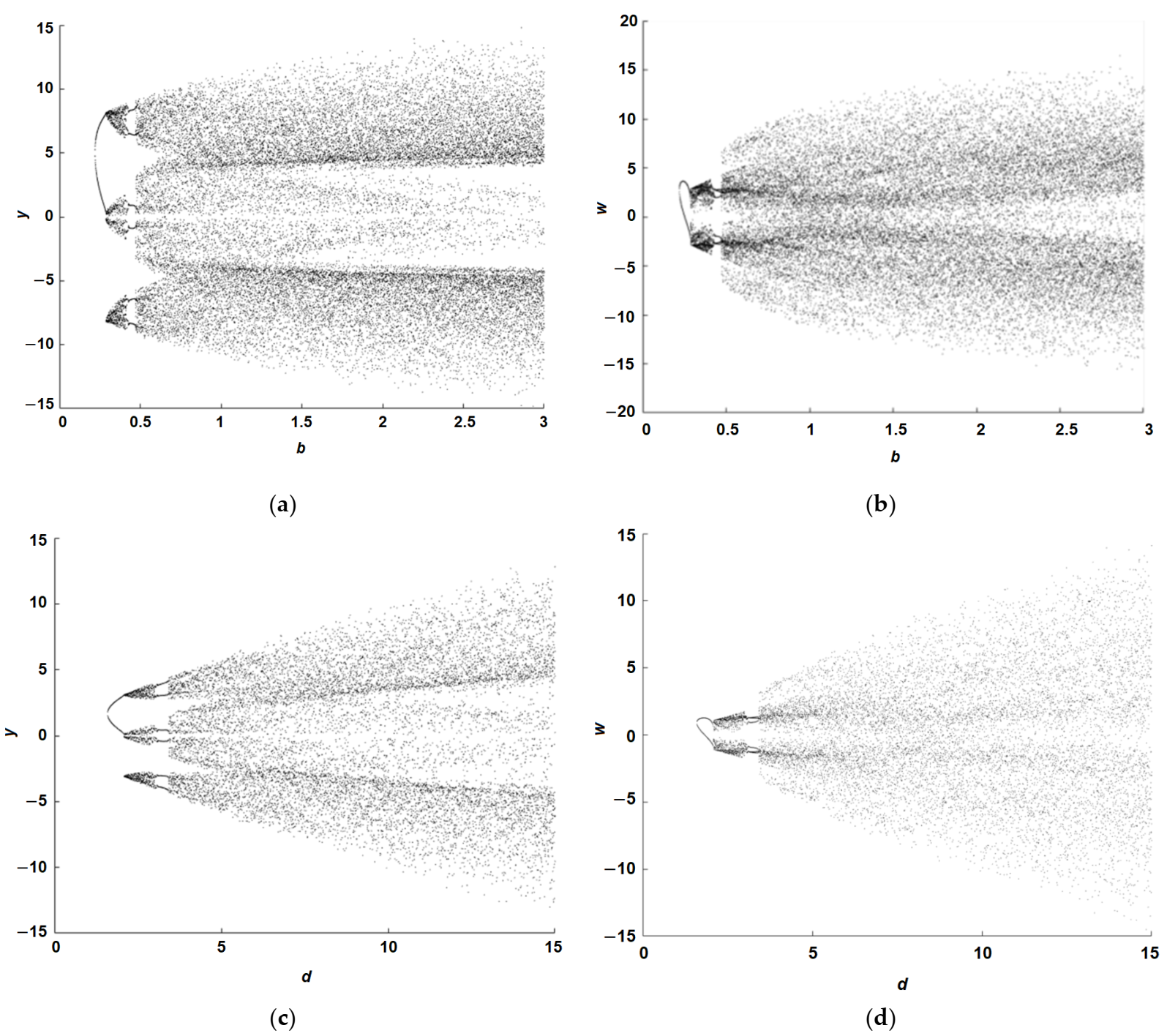
2.3. Bicurcation Analysis

Figure 1 shows the bifurcation diagram of system (1) with different values of parameter b and d versus y and w state variables by using the initial conditions x₀ = y₀ = z₀ = w₀ = 1.

2.4. Lyapunov Exponents

The behavior of Lyapunov exponents is shown in Figure 2. The initial conditions x₀ = y₀ = z₀ = w₀ = 1 and parameter d = 14.5, are considered. Figure 2 shows evolution of Lyapunov exponents L₁ = 0.5841, L₂ = 0.000127664, L₃ = −0.4873, and L₄ = −3.5968 considering the variation of bifurcation parameter d = [1.5–15]; the system (1) exhibits two positive Lyapunov exponents L₁, L₂ > 0, which means that NHS has hyperchaotic behavior.

The fractal dimension, commonly known as the Kaplan-Yorke dimension D_KY, of this system is:

$$\begin{array}{c}{D}_{KY}=j +\frac{1}{\left|L_{j+1}\right|}{{\displaystyle \sum }}_{i=1}^j{L}_i=3+\frac{L_1{+L }_2{+L}_3}{\left|L_4\right|}\\ D_{KY}= 3 +\frac{0.5841+0.000127664-0.4873}{\left|-3.5968\right|}=3.0269.\end{array}$$

(9)

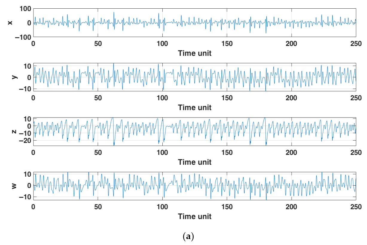
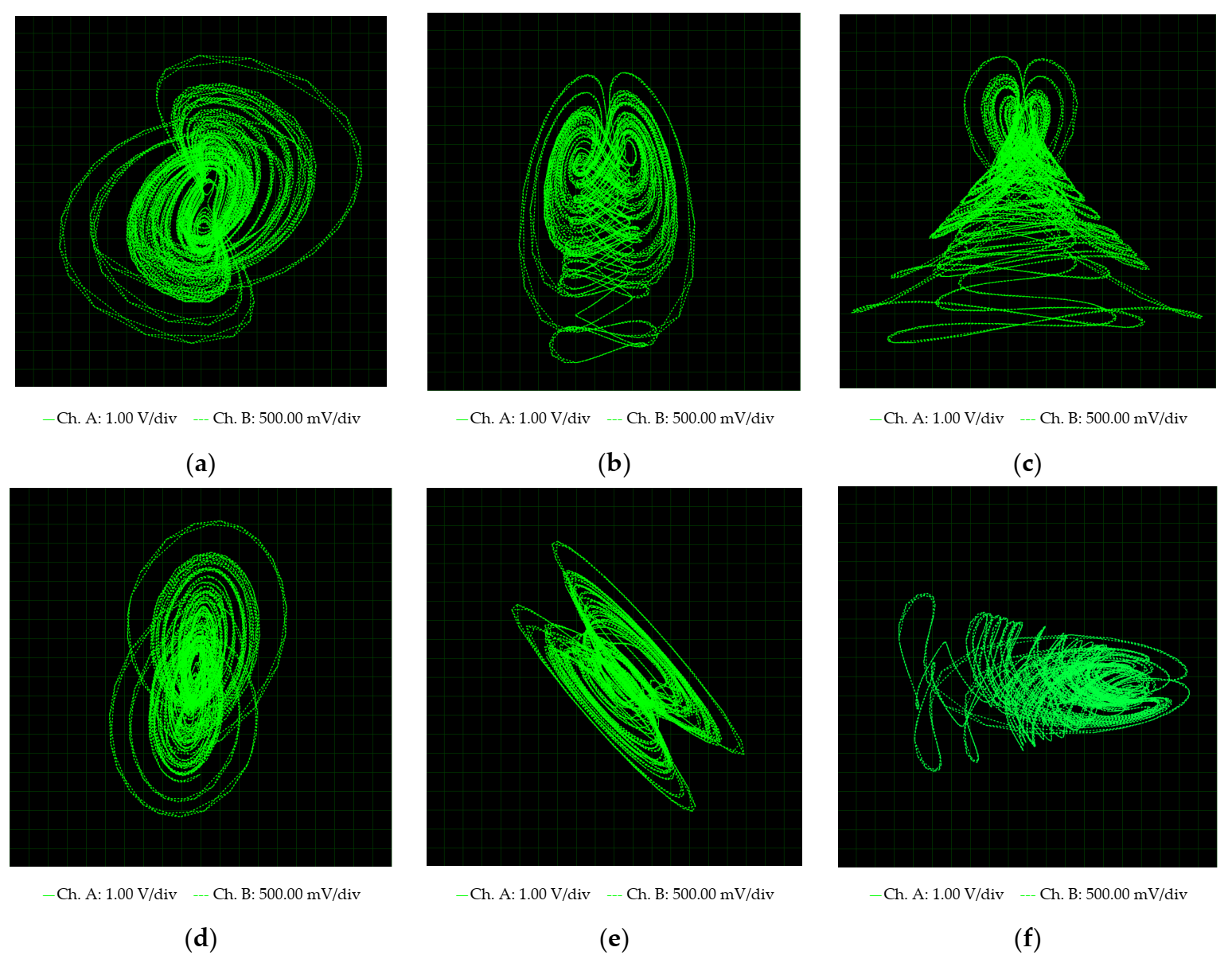
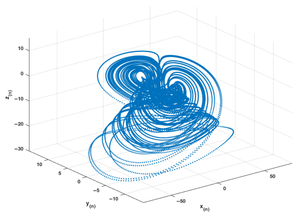
2.5. Numerical Simulations

Figure 3 shows the temporary states x, y, z, and w, the phase planes and phase space with the strange attractor of system (1) by using the initial conditions x₀ = y₀ = z₀ = w₀ = 1 and the parameters a = 2, b = 2, c = 0.5, and d = 14.5.

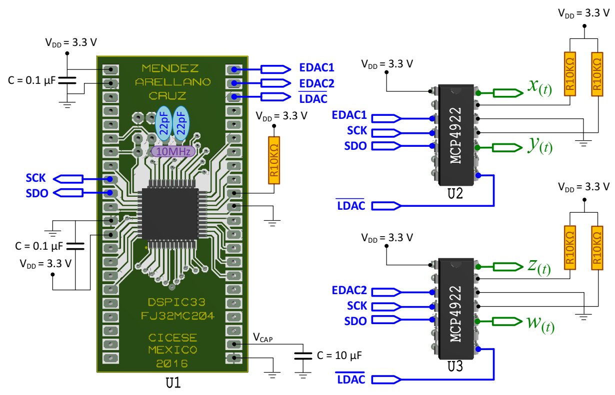
3. Electronic Implementations

In this section, the electronic simulation and implementation of the NHS are presented in their continuous and discretized versions. All the hardware simulation used in NHS are conducted using the Proteus Virtual System Modeling (VSM) software. The continuous version was implemented by means of a circuit designed using TL84 operational amplifiers [32,34]. The discretized version was conducted using the Proteus VSM which has Microchip libraries that include the 16-bit dsPIC33FJ microcontroller and external DACs, the numerical and experimental methods, described in [26,32], are carried out in the electronic implementation of the discretized versions of NHS in floating-point and fixed-point Q1.15.

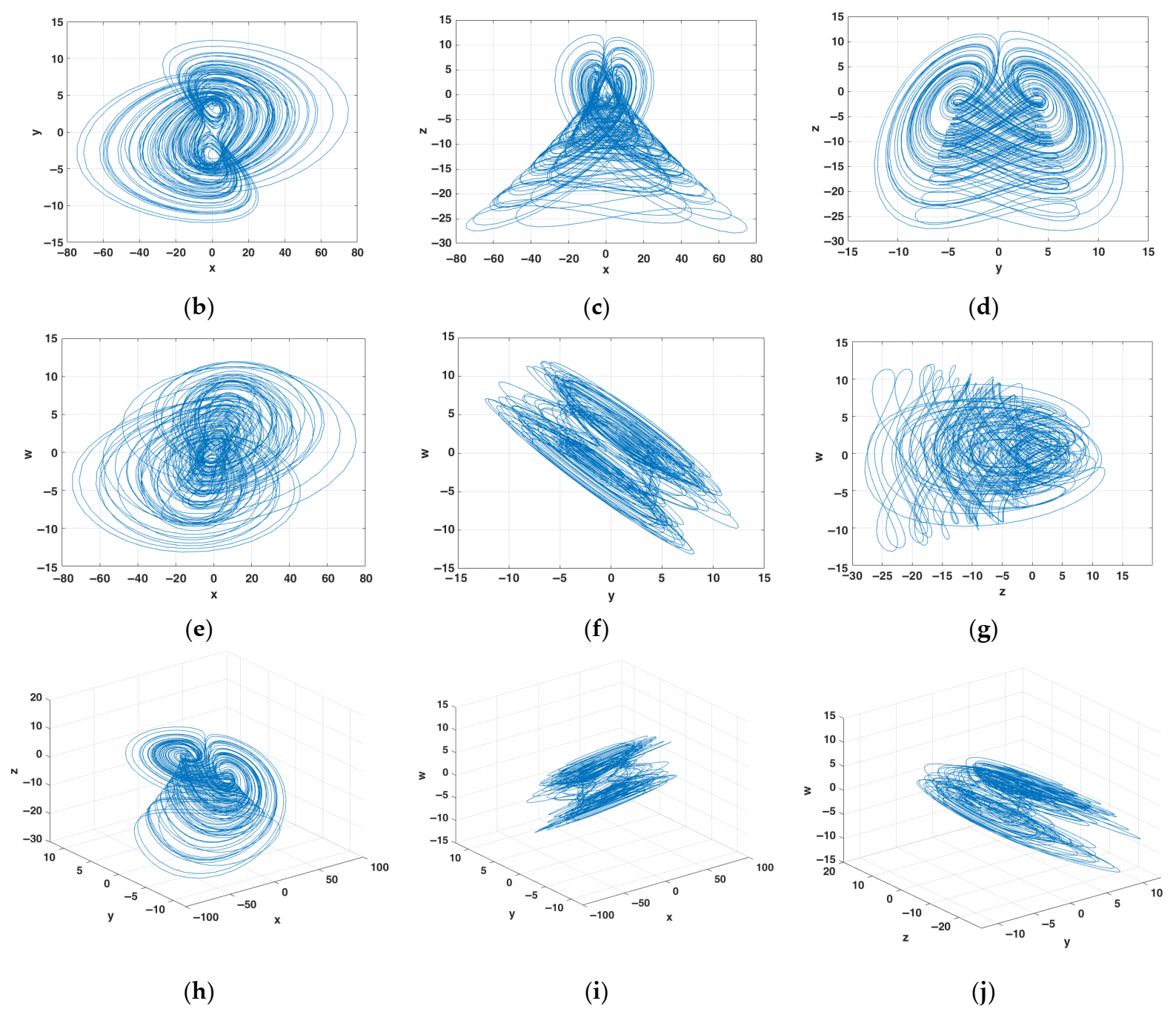
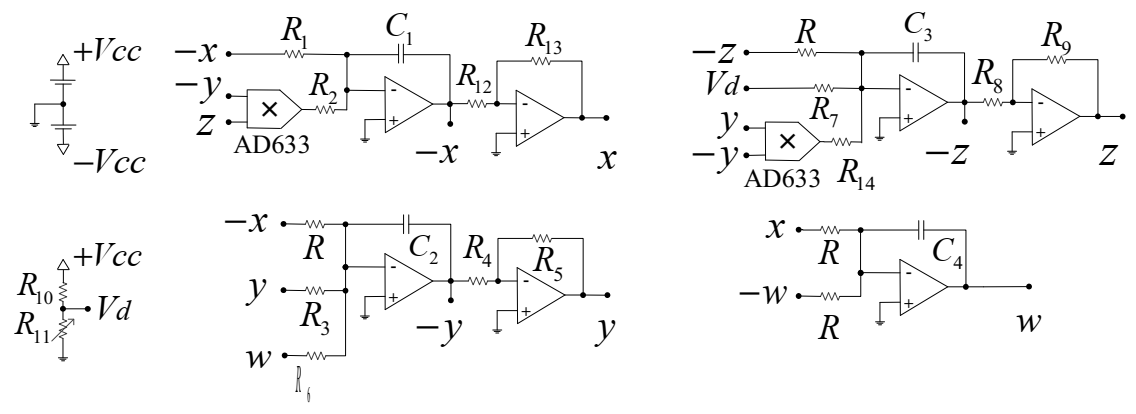
3.1. Continuous Version and Its Electronic Circuit Design

To implement the electronic continuous version of system (1), the normalized model is regarding with the attenuation factor of 20 for each state variables, i.e., x = 20o, y = 20p, z = 20q, w = 20r are defined. Replacing the new variables on system (1), we obtain the following system:

$$\begin{array}{l}\dot{o}=-2o - 40pq,\\ \dot{p}=-o+0.5p+0.5r,\\ \dot{q}=0.725 -{ 20p}^2-q,\\ \dot{r}=o- r.\end{array}$$

(10)

Replacing the state variables again for o = x, p = y, q = z, r = w, the circuit equivalent representation of system (10) is defined by

$$\begin{array}{l}\dot{x}=\frac{1}{{RC}_1}\left(-\frac{R}{R_1}x -\frac{R}{{10R}_{10}}yz\right),\\ \dot{y}=\frac{1}{{RC}_2}\left(-x+\frac{R}{R_5}y+\frac{R}{R_5}w\right),\\ \dot{z}=\frac{1}{{RC}_3}\left(-\frac{R}{R_9}b -\frac{R}{{10R}_8}{y}^2- z\right),\\ \dot{w}=-\frac{1}{{RC}_4}\left(-x+w\right),\end{array}$$

(11)

where the values of components are: C₁ = C₂ = C₃ = C₄ = 100 pF, R = R₇ = 1 MΩ, R₁₀ = 1 MΩ R₁ = 500 kΩ, R₄ = R₅ = R₈ = R₉ = R₁₂ = R₁₃ = 10 kΩ, R₁₄ = 94 kΩ, R₂ = 47 kΩ, R₃ = R₆ = 2 MΩ, the control parameter is fixed in d = 14.5 with R₁₁ = 4.2 MΩ, and the circuit (10) is supply with +Vcc = 18 V and −Vcc = −18 V. To see a change in the dynamical behavior of system (10), is recommend represent the critical parameter d with a variable resistor to R_11(VAR) = [0–5 MΩ]. The electronic version of system (11) is implemented using operational amplifiers TL084 and multipliers AD633. Figure 4 shows the equivalent circuit of system (11).

In order to compare the experimental results of the system (11), Figure 5 shows the electronics implementation using Proteus VSM simulation and Figure 6 shows the electronic circuit implementation assembly shown in Figure 4. We can see that the corresponding attractors are highly similar with respect to those shown in Figure 3.

3.2. Discretized Version and Embedded System Design

The Euler’s method allows discretizing a continuous system, which is derived from the expansion of Taylor’s series where the quadratic and upper order term are truncated. The Euler method is used to approximate the ordinary differential equations (ODEs) and it is described by

$$\begin{array}{l}\dot{\mathbf{x}}=\mathbf{f}\left(\mathbf{x}\right),\\ \mathbf{x}\left(0\right) ={\mathbf{x}}_0\\ \mathbf{x}\in {\mathbb{R}}^N\end{array}$$

(12)

is given by

x_{(n + 1)} = x_(n) + τf(x_(n)),

(13)

where τ is the step size and n is the iteration that represents the time in discrete version. The Matlab simulations are carried out using the same parameter and initial conditions (i.e., x₀ = y₀ = z₀ = w₀ = 1) considering τ = 0.005 and n = 30000. The Euler algorithm requires less arithmetic operations because it presents just one step, and it is easy to implement [35]. The Euler’s discretization (13) is used to represent the DV of system (1) as follows

x_{(n + 1)} = x_(n) + τ(−ax_(n) − by_(n)z_(n)),
y_{(n + 1)} = y_(n) + τ(−x_(n) + cy_(n) + cw_(n)),
z_{(n + 1)} = z_(n) + τ(d − y_(n)² − z_(n)),
w_{(n + 1)} = w_(n) + τ(x_(n) − w_(n)).

(14)

Figure 7 shows phase space simulation x_(n) versus y_(n) versus z_(n) of discretized system (14).

3.2.1. Circuit Design of an Embedded System

An important attribute of Matlab software and Mikro C for dsPIC compiler is that both have the IEEE-754 standard, numerical results are equivalent to represents the simulation and implementation of the discretized system (14), the numerical data are implemented in 16-bits floating-point format, and fixed-point Q1.15 [36]. The dsPIC architecture allows fast calculation in comparison with 16-bit microcontrollers because it has a DSP engine, therefore it is an important attribute for the implementation of this embedded system.

Table 2. Data bus description of embedded system (ES).

Peripheral Number	Hardware Description
U1	Master, microcontroller dsPIC33FJ32MC204
U2	Slave 1, DAC MCP4922 shows x(t) and y(t)
U3	Slave 2, DAC MCP4922 shows z(t) and w(t)

describes the peripherals used for this embedded system, where all operations are performed by a 16-bit dsPIC microcontroller dsPIC33FJ and DACs MCP4922 (Microchip Technology, Chandler, AZ, USA) with multiple output of 12-bit resolution, both are energized with Vdd = Vcc = 3.3 V.

In the ES implementation, the SPI protocol is used because it contemplates easy configuration using low-quantity lines and fast serial data bus transmission with the external peripherals. U1 is configured as a master mode, and U2 and U3 as slave, the data serial is 16-bit mode and quick communication of 16.6 Mbps.

The data bus description of the embedded system is described in

Table 3. Data bus description of ES.

U1 Pin	Description
RB14—SCK	Serial clock signal to synchronize U2 and U3
RB13—SDO	Serial data output to enable U2 and U3
RC2—EDAC1	Chip Select to enable U2
RC1—EDAC2	Chip Select to enable U3
RC0—LDAC	Enable U2–U3 simultaneously to depict the state variables x(n), y(n), z(n), and w(n)

. From U1, the control lines SDO, SCK, EDAC1, EDAC2, and LDAC are generated to control U2 and U3 for depict the state variables x_(n), y_(n), z_(n), and w_(n) synchronized for each n iteration. The schematic circuit design of the embedded system is shown in Figure 8.

The maximum number of n iterations generated in one second is referred to the total quantity of iterations Q_T, and it is represented in time units (tu), the NHS has four dimensions, i.e., N = 4 dimensions, and the Q_T representation is given by

$$Q_{\mathrm{T}}{=\tau f}_{\mathrm{Td}}=\tau \frac{1}{T_{\mathrm{Td}}}=\tau \frac{1}{t_{\mathrm{c}}{+t}_{\mathrm{Tg}}}=\tau \frac{1}{t_{\mathrm{c}}+{{\displaystyle \sum }}_{j=1}^N{t}_{\mathrm{Tdac}\left(j\right)}},$$

(15)

where the time period T_Td is considered as the total-decoding-time that the algorithm needs to reproduce an iteration n, and f_Td represents the maximum number of iterations n that the ES generates in one second (ips); the frequency f_Td is the reciprocal of T_Td. The time complexity t_c is the time that numerical algorithm (NA) needs to reproduce one iteration n by using U1; the total-graphic time t_Tg is the time that the two DACs U2–U3 required to represent the four state variables x_(t), y_(t), and z_(t), w_(t), respectively. The t_Tdac is the time required for each DAC which represents two state variables, and the ES design illustrates, at the same time, the state variables x_(t), y_(t), z_(t), and w_(t) for each n sample.

In the next subsection we will analyze two electronic implementations, using a numerical format for each. Specifically, we are using the proposed parameters of Equation (15) to denote the system (14) in floating-point with the sub index 1, and the same system (14)—with some numerical variable changes—in fixed-point with the sub index 2.

3.2.2. Implementation of the DV of NHS in Floating-Point

The flow chart of the electronic/digital implementation process of the DV of NHS (14) is shown in Figure 9. The description of each step is described below.

From Figure 9, the steps 1–3 describe the process to set the numerical conditions to initialize the ports, system libraries, variables, parameters, and set the initial conditions of the DV of NHS (14) in floating-point. Subsequently, the steps 4–6 describe all the entire loop-process to store, and rescaling the state variables in positive scale. Finally, the steps 7–8 describe the rescaling process to write the U2 and U3 DACs of the system (14) for specific n iteration.

Figure 10 and

Table 4. Implementation results of DV-system (14) on the proposed ES.

Parameter	Result
τ	0.02
tc1	56 µs
tTg1	34.4 µs
TTd1	90.4 µs
fTd1	11061 ips
QT1	221.22 tu

show the implementation results of the DV of the NHS (14) to exemplify (15). We obtained Q_T1 = 221.22 considering τ = 0.02 using the proposed ES.

This study is focused on computing the numerical results, considering only the capability that the embedded system has to run the NA of system (14) and dismissing the graphic results t_Tg1 = 0, which means that only can be considered t_c1 = 56 µs—the numerical conversions to set and write the 12-bit DACs U2 and U3 are ignored, and the algorithm (14) is only implemented in U1. We obtained T_Td1 = 56 µs, which means that the NA has a performance of f_Td1 = 17857 ips.

3.2.3. Implementation of the DV of NHS in Fixed-Point Q1.15

The dsPIC microcontroller includes DSP proficiencies; it is a 16-bit microcontroller with high-performance and a high computation speed. The DSP libraries of MikroC PRO for dsPIC Compiler (MikroElektronika, Belgrade, Serbia) are based on fixed-point, and their routines work with fractional Q1.15 format [35]. The coefficients, the step size, and state variables of discretized system (14) must be arrangement in fractional Q1.15 format to not excess the numerical limits (−1, 1). The same numerical attenuation used in system (10) and electronics implementation of system (11) is used in the DV of system (14). The attenuation factor 20 is proposed for each x = 20o, y = 20p, z = 20q, and w = 20r state variables, replacing in system (14), the following system is obtained,

o_{(n + 1)} = o_(n) − aτo_(n) − bτp_(n)q_(n),
p_{(n + 1)} = p_(n) − τo _(n) + cτp_(n) + cτr_(n),
q_{(n + 1)} = q_(n) + dτ − τp_(n)² − τq_(n),
r_{(n + 1)} = r_(n) + τo _(n) − τr_(n),

(16)

evaluating τ = 0.02, and with the corresponding parameters, we have

o_{(n + 1)} = 0.96o_(n) − 0.8p_(n)q_(n),
p_{(n + 1)} = − 0.02o_(n) + 0.505p_(n) + 0.505p_(n) + 0.01r_(n),
q_{(n + 1)} = 0.0145 + 0.98q_(n) − 0.4p_(n)²,
r_{(n + 1)} = 0.02o _(n) + 0.98r_(n).

(17)

The vector multiplication function and vector dot function of the DSP system libraries are used to build the algorithm of system (17). First, the vector dot function is used to multiply the two nonlinearities p_(n)q_(n) and p_(n)² by separation, after the vector dot function is used for the representation of each equation of the DV of system (17), the results obtained are represented in fixed-point Q1.15. In Figure 11, we illustrate the flow chart of the electronic/digital implementation process of the DV of NHS (17), the steps 1–3 describe the process to set the numerical conditions to initialize the ports, system libraries, variables, parameters, and set the initial conditions converted in fixed-point. Subsequently, the steps 4–6 describe all the entire loop-process to store and rescale the state variables in a positive scale. Finally, steps 7–8 describe the rescaling process to write the U2 and U3 DACs of the system (17) for specific n iteration.

Figure 12 and

Table 5. Implementation results in fixed-point of the DV of system (17) on the proposed ES.

Parameter	Result
τ	0.02
tc2	6 µs
tTg2	34.4 µs
TTd2	40.4 µs
fTd2	24752 ips
QT2	495.04 tu

show the implementation results in fixed-point of the DV of the NHS (17) to exemplify (15). We obtained more Q_T2 = 495.04, considering the same τ = 0.02 from system (14) and implementing it in the proposed ES.

The system (17) is implemented in the embedded system and the graphic results are dismissed t_Tg2 = 0, which means that only t_c2 = 6 µs is computed. We obtained T_Td2 = 6 µs, which means that the NA has a performance of f_Td2 = 166666 ips.

3.2.4. Comparison of the Digital Implementations of the DV of NHS Algorithm in dsPIC

For better comparison between the performance algorithms of the DV of the NHS in the dsPIC,

Table 6. Implementation results of the DV of NHS system (14) versus DV of system NHS (17) on the ES.

Parameter	Floating-Point System (14) Result	Fixed-Point System (17) Result
τ	0.02	0.02
tc	56 µs	6 µs
tTg	34.4 µs	34.4 µs
TTd	90.4 µs	40.4 µs
fTd	11061 ips	24752 ips
QT	221.22 tu	495.04 tu

summarizes the electronic implementation using the ES with different numerical representation of system (14) and system (17), in Table 4 and Table 5, respectively. The electronic implementation of system (17) is based on Q1.15 fixed-format and it shows better T_Td2 = 6 µs and f_Td2 = 166666 ips performance versus the floating-point format used in the system (14), which shows T_Td1 = 56 µs and f_Td1 = 17857 ips, which means that there is 89% improvement in the ips reproduction by using the same algorithm.

The proposed hardware of the ES allows comparison of the performance of the system algorithm (14) versus the system algorithm (17). The algorithm of the system (17) was based on the fixed-point format Q1.15, and it had better performance for digital applications because it provides 166.6 kHz iterations per second, which means that it is very attractive as a base system for encryption applications and electronics implementations, e.g., to encrypt high-fidelity audio such as Compact Disk quality 44.1 kHz or DVD audio quality 48 kHz, data-transfer, and even for low-resolution video applications or image, among others.

4. Conclusions

This work presented analytical and numerical studies of a new hyperchaotic system (NHS) that produces chaos and hyperchaos, varying only two parameters. The analysis includes tests of symmetry, dissipativity, equilibria and stability, bifurcation analysis, and Lyapunov exponents. The results showed that new hyperchaotic attractor presents two positive Lyapunov exponents, an unstable equilibrium saddle-point at the origin, and it is flexible and robust which allows obtaining different hyperchaotic and chaotic behavior.

The simulation results of the NHS in its continuous version (CV) and discretized version (DV) were conducted using Proteus Virtual System Modeling (VSM), and the experimental electronic results were carried out using operational amplifiers for CV. In addition, a novel study to implement the DV of the NHS in an embedded system was presented, which is very useful in digital implementation. In general, we can mention that the digital implementation has some benefits versus the electronic implementation of the analog systems, which is the typical aging, and tolerance of the components, which means that chaotic systems are highly attractive in the electronic digital implementation if the chaos quality condition is preserved.

The ES has a simple hardware design, easy connection with low-cost of implementation (only $6 USD dsPIC33FJ plus two DACs 4922) and is friendly for digital electronic implementation. The DSP-engine numerical properties of the dsPIC microcontroller allowed validation of the numerical performance of the DV of the NHS, and its algorithm was implemented and compared in floating-point versus fractional Q1.15 versions. The Q1.15 fractional version showed very good performance in the DV of NHS, it has the capability to run over 166k iteration per second (ips), and it is very attractive as a main algorithm, e.g., to implement a digital cryptosystem based in chaos, where a high quantity of iteration per second is essential to encrypt multimedia applications and to transfer cryptograms of digital audio of high fidelity, files, pictures, or even compressed video of low-resolution.

As future work, complementary studies will carry out the NHS with encryption and synchronization applications. Other techniques for representation of discretized version will be incorporated as the fractional and fixed-point computation on an embedded system in 32-bit microcontroller.

References

1. Eckmann, J.-P.; Ruelle, D. Ergodic theory of chaos and strange attractors. Rev. Mod. Phys. 1985, 57, 617–656. [Google Scholar] [CrossRef]
2. May, R.M. Simple mathematical models with very complicated dynamics. Nature 1976, 261, 459–467. [Google Scholar] [CrossRef] [PubMed]
3. Alligood, K.T.; Sauer, T.D.; Yorke, J.A. Chaos: An Introduction to Dynamical Systems; Springer: Berlin, Germany, 1996. [Google Scholar]
4. Strogatz, S.H. Nonlinear Dynamics and Chaos: With Applications to Physics, Biology, Chemistry, and Engineering; Perseus Books: Boston, MA, USA, 1994. [Google Scholar]
5. Liu, J.; Wang, Z.; Shu, M.; Zhang, F.; Leng, S.; Sun, X. Secure Communication of Fractional Complex Chaotic Systems Based on Fractional Difference Function Synchronization. Complexity 2019, 2019, 7242791. [Google Scholar] [CrossRef] [Green Version]
6. Nakamura, Y.; Sekiguchi, A. The chaotic mobile robot. IEEE Trans. Robot. Autom. 2001, 17, 898–904. [Google Scholar] [CrossRef]
7. Arellano-Delgado, A.; López-Gutiérrez, R.; Cruz-Hernández, C.; Posadas-Castillo, C.; Cardoza-Avendaño, L.; Serrano-Guerrero, H. Experimental network synchronization via plastic optical fiber. Opt. Fiber Technol. 2016, 19, 93–98. [Google Scholar] [CrossRef]
8. Murillo-Escobar, M.A.; Cruz-Hernández, C.; Abundiz-Pérez, F.; López-Gutiérrez, R.M. A robust embedded biometric authentication system based on fingerprint and chaotic encryption. Expert Syst. Appl. 2015, 42, 8198–8211. [Google Scholar] [CrossRef]
9. Méndez-Ramírez, R.; Arellano-Delgado, A.; Cruz-Hernández, C.; Abundiz-Perez, F.; Martinez-Clark, R. Chaotic digital cryptosystem by using SPI protocol and its dsPICs implementation. Front. Inf. Technol. Electron. Eng. 2018, 19, 165–179. [Google Scholar] [CrossRef]
10. Méndez-Ramírez, R.; Arellano-Delgado, A.; Murillo-Escobar, M.; Cruz-Hernández, C. Multimedia contents encryption using the chaotic MACM system on a smart-display. In Cryptographic and Information Security Approaches for Images and Videos; CRC Press Taylor & Francis Group: Boca Raton, FL, USA, 2019; 10th chapter. [Google Scholar]
11. Lorenz, E. Deterministic nonperiodic flow. J. Atmos. Sci. 1963, 20, 130–141. [Google Scholar] [CrossRef] [Green Version]
12. Rössler, O.E. An equation for continuous chaos. Phys. Lett. A 1976, 57, 397–398. [Google Scholar] [CrossRef]
13. Rössler, O.E. An equation for Hyperchaos. Phys. Lett. A 1979, 71, 155–157. [Google Scholar] [CrossRef]
14. Vaidyanathan, S.; Rajagopal, K.; Sambas, A.; Kacar, S.; Cavusoglu, U. A new hyperchaotic temperature fluctuations model, its circuit simulation, FPGA implementation and an application to image encryption. Int. J. Simul. Process. Model. 2018, 13, 281–296. [Google Scholar] [CrossRef]
15. Kamdem Kuate, P.D.; Lai, Q.; Fotsin, H. Complex behaviors in a new 4D memristive hyperchaotic system without equilibrium and its microcontroller-based implementation. Eur. Phys. J. Spec. Top. 2019, 228, 2171–2184. [Google Scholar] [CrossRef]
16. Rajagopal, K.; Vaidyanathan, S.; Karthikeyan, A.; Srinivasan, A. Complex novel 4D memristor hyperchaotic system and its synchronization using adaptive sliding mode control. Alex. Eng. J. 2018, 57, 683–694. [Google Scholar] [CrossRef]
17. Rajagopal, K.; Karthikeyan, A.; Duraisamy, P. Hyperchaotic Chameleon: Fractional Order FPGA Implementation. Complexity 2017, 16, 8979408. [Google Scholar] [CrossRef] [Green Version]
18. Vicente, R.; Daudén, J.; Colet, P.R. Toral Analysis and Characterization of the Hyperchaos Generated by a Semiconductor Laser Subject to a Delayed Feedback Loop. IEEE J. Quantum Electron. 2005, 41, 541–548. [Google Scholar] [CrossRef] [Green Version]
19. Panga, S.; Liu, Y. A new hyperchaotic system from the Lü system and its control. J. Comput. Appl. Math. 2011, 235, 2775–2789. [Google Scholar] [CrossRef] [Green Version]
20. Li-Xin, J.; Hao, D.; Meng, H. A new four-dimensional hyperchaotic Chen system and its generalized synchronization. Chin. Phys. B 2010, 19, 100501. [Google Scholar] [CrossRef]
21. Ding, L.; Ding, Q. A Novel Image Encryption Scheme Based on 2D Fractional Chaotic Map, DWT and 4D Hyper-chaos. Electronics 2020, 9, 1280. [Google Scholar] [CrossRef]
22. Kapitaniak, T.; Maistrenko, Y.; Popovych, S. Chaos-hyperchaos transition. Phys. Rev. E 2000, 62, 1972. [Google Scholar] [CrossRef] [Green Version]
23. Li, G.L.; Chen, X.Y.; Liu, F.C.; Mu, X.M. Hyper-chaotic Canonical 4-D Chua’s Circuit. In Proceedings of the 2009 International Conference on Communications, Circuits and Systems, Milpitas, CA, USA, 23–25 July 2009; p. 10879007. [Google Scholar]
24. Wang, X.; Wang, M. A hyperchaos generated from Lorenz system. Phys. A Stat. Mech. Appl. 2008, 387, 3751–3758. [Google Scholar] [CrossRef]
25. Chen, B.; Yu, S.; Chen, P.; Xiao, L. Design and Virtex-7-Based Implementation of Video Chaotic Secure Communications. Int. J. Bifurc. Chaos 2020, 30, 24. [Google Scholar] [CrossRef]
26. Méndez-Ramírez, R.; Arellano-Delgado, A.; Murillo-Escobar, M.; Cruz-Hernández, C. Degradation Analysis of Chaotic Systems and their Digital Implementation in Embedded Systems. Complexity 2019, 22, 9863982. [Google Scholar] [CrossRef] [Green Version]
27. Zhang, L. Fixed-point FPGA model-based design and optimization for Henon map chaotic generator. In Proceedings of the 2017 IEEE 8th Latin American Symposium on Circuits & Systems (LASCAS), Bariloche, Argentina, 20–23 February 2017; p. 16964391. [Google Scholar]
28. Flores-Vergara, A.; Inzunza-González, E.; García-Guerrero, E.E.; López-Bonilla, O.; Rodríguez-Orozco, E.; Hernández-Ontiveros, J.M.; Cárdenas-Valdez, J.R.; Tlelo-Cuautle, E. Implementing a Chaotic Cryptosystem by Performing Parallel Computing on Embedded Systems with Multiprocessors. Entropy 2019, 21, 268. [Google Scholar] [CrossRef] [Green Version]
29. Chuan Qin, K.S.; Shaobo, H. Characteristic Analysis of Fractional-Order Memristor-Based Hypogenetic Jerk System and Its DSP Implementation. Electronics 2021, 10, 841. [Google Scholar] [CrossRef]
30. Mendez-Ramirez, R.; Arellano-Delgado, A.; Cruz-Hernandez, C.; Lopez-Gutierrez, R.M. Degradation analysis of generalized Chua’s circuit generator of multi-scroll chaotic attractors and its implementation on PIC32. In Proceedings of the Future Technologies Conference (FTC), San Francisco, CA, USA, 6–7 December 2016; pp. 1034–1039. [Google Scholar]
31. Koulamas, C.; Lazarescu, M.T. Real-Time Embedded Systems: Present and Future. Electronics 2018, 7, 205. [Google Scholar] [CrossRef] [Green Version]
32. Méndez-Ramírez, R.; Cruz-Hernández, C.; Arellano-Delgado, A.; Martínez-Clark, R. A new simple chaotic Lorenz-type system and its digital realization using a TFT touch-screen display embedded system. Complexity 2017, 2017, 6820492. [Google Scholar] [CrossRef] [Green Version]
33. Nik, H.S.; Golchaman, M. Chaos Control of a Bounded 4D Chaotic System. Neural Comput. Applic. 2014, 25, 683–692. [Google Scholar]
34. Qinghai, S.; Hui, C.; Yuxia, L. Complex Dynamics of a Novel Chaotic System Based on an Active Memristor. Electronics 2020, 9, 410. [Google Scholar] [CrossRef] [Green Version]
35. Yang, W.Y.; Cao, W.; Chung, T.-S.; Morris, J. Applied Numerical Methods Using Matlab; John Wiley and Sons Inc.: Hoboken, NJ, USA, 2005. [Google Scholar]
36. Microchip Technology Inc. 16-Bit Language Tools Libraries, Reference Manual; Microchip Technology Inc.: Chandler, AZ, USA, 2014; DS0001456J.1–155. [Google Scholar]
Figure 1. Bifurcation diagrams of parameters b and d: (a) b versus y state with variations of b = [0.1–3], (b) b versus w state with variations of b = [0.1–3]. (c) d versus y state with variations of d = [1.5–15], and (d) d versus w state with variations of d = [1.5–15].
Electronics 10 01793 g001
Figure 2. Lyapunov exponents of system (1) with the variation of bifurcation parameter d = [14–15].
Electronics 10 01793 g002
Figure 3. Hyperchaotic attractor of system (1): (a) time evolution of states x, y, z and w; (b) phase plane x versus y; (c) phase plane x versus z; (d) phase plane y versus z; (e) phase plane x versus w; (f) phase plane y versus w; (g) phase plane z versus w; (h) phase space x versus y versus z; (i) phase space x versus y versus w; and (j) phase space y versus z versus w.
Electronics 10 01793 g003aElectronics 10 01793 g003b
Figure 4. Schematic diagram of the equivalent circuit of system (11).
Electronics 10 01793 g004
Figure 5. Electronic simulation of system (11) using Proteus VSM: (a) phase plane x versus y; (b) phase plane x versus z; (c) phase plane y versus z; (d) phase plane x versus w; (e) phase plane y versus w; (f) phase plane z versus w.
Electronics 10 01793 g005
Figure 6. Electronic circuit implementation of system (11): (a) phase plane x versus y; (b) phase plane x versus z; (c) phase plane y versus z; (d) phase plane x versus w; (e) phase plane y versus w; (f) phase plane z versus w.
Electronics 10 01793 g006
Figure 7. Hyperchaotic attractor of DV-system (14) projected on x(n) versus y(n) versus z(n).
Electronics 10 01793 g007
Figure 8. Schematic of the implementation of system (14) in embedded system.
Electronics 10 01793 g008
Figure 9. Flow chart of the electronic/digital implementation process in floating-point version of NHS (14).
Electronics 10 01793 g009
Figure 10. Electronic circuit implementation of system (11): (a) phase plane x(n) versus y(n); (b) phase plane x(n) versus z(n); (c) phase plane y(n) versus z(n); (d) phase plane x(n) versus w(n); (e) phase plane y(n) versus w(n); (f) phase plane z(n) versus w(n).
Electronics 10 01793 g010
Figure 11. Flow chart of the electronic/digital implementation process in Q1.15 fixed-point version of NHS (17).
Electronics 10 01793 g011
Figure 12. Hyperchaotic system (17) implemented in fixed-point: (a) time evolution of states z(n) and w(n); (b) phase plane z(n) versus w(n).
Electronics 10 01793 g012