Robust Tracker of Hybrid Microgrids by the Invariant-Ellipsoid Set

Abstract

This paper introduces a new ellipsoidal-based tracker design to control a grid-connected hybrid direct current/alternating current (DC/AC) microgrid (MG). The proposed controller is robust against both parameters and load variations. The studied hybrid MG is modelled as a nonlinear dynamical system. A linearized model around an operating point is developed. The parameter changes are modelled as norm-bounded uncertainties. We apply the new extended version of the attractive (or invariant) ellipsoid for this tracking problem. Convex optimization is used to obtain the region’s minimal size where the tracking error between the state trajectories and the reference states converges. The sufficient conditions for stability are derived and solved based on linear matrix inequalities (LMIs). The proposed controller’s validity is shown via simulating the hybrid MG with various operational scenarios. In each scenario, the performance of the controller is compared with a recently proposed sliding mode controller. The comparison clearly illustrates the superiority of the developed controller in terms of transient and steady-state responses.

1. Introduction

Technology advances in power generation, control, computer hardware, and software have led to the spread of microgrids (MGs). Industrial customers aiming to reduce the cost and increase their reliability and resilience have driven the MGs’ evolution. As a result, the MGs are currently the primary power source for many commercial and residential applications [1].

Locality, independence, and intelligence are the key characteristics of the MG. The MG’s locality provides an optimal solution to the power losses issue of a typical power system structure, reaching up to 40% of the generated power. In many cases, the MG is the only solution to the power supply of remote areas where the public grid is inaccessible or does not exist [2].

MGs’ independence is attributed to their ability to supply the total load demand in the outage of the utility services or the existence of severe disturbances. The MG can operate synchronously with the utility grid or in isolated mode. When isolated, it can completely control its voltage and frequency, thanks to the dedicated power converters and their advanced control schemes [3].

Embedded sensors, communications channels, innovative software, and powerful controllers have instigated MG’s intelligence. Intelligence in this context implies the capability of self-monitoring, evaluation, and decision-making to optimally utilize and operate the available energy resources in addition to the energy-management system [4].

MG’s installation and commissioning are soaring. For instance, in 2019 (second half only), there were 4475 projects adding up to 27 GW of installed capacity [5]. California State, USA, has demonstrated great impetus to obtain 50% of its electricity via MGs and renewable sources by 2030 [6]. MGs’ development in the European Union Nations, Japan, Korea, Australia, and North America is reported in [7], showing explicitly that the implementations are growing rapidly.

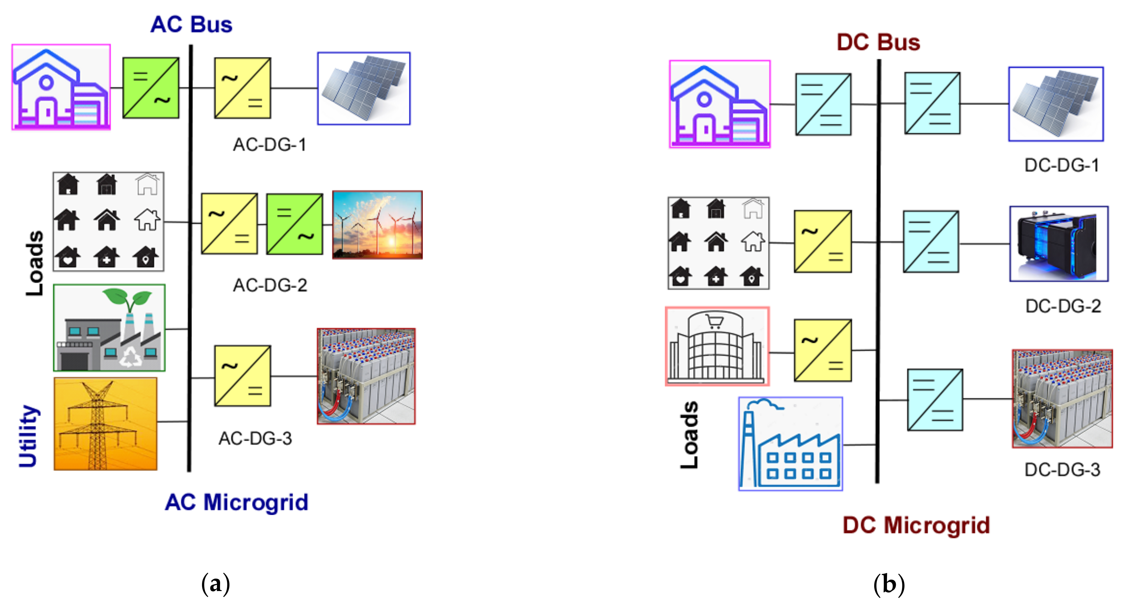
Based on the integration level into the primary grid, the MGs are classified into a remote-, facility- and utility-MG, ordered by their impact on the power system from low to high. The MG can be a direct current (DC), alternating current (AC), or hybrid system. Figure 1a displays a layout example of an AC MG, and Figure 1b depicts an outline of a DC MG. Statistically, the AC-MG system configuration is still dominant due to mainly two factors: AC-load availability and ease of protection [8]. However, some factors push the DC MG to compete with the AC MG, such as the DC-based renewable system’s spread and ease of control. A hybrid MG aims to merge the merits of both systems [9,10]. 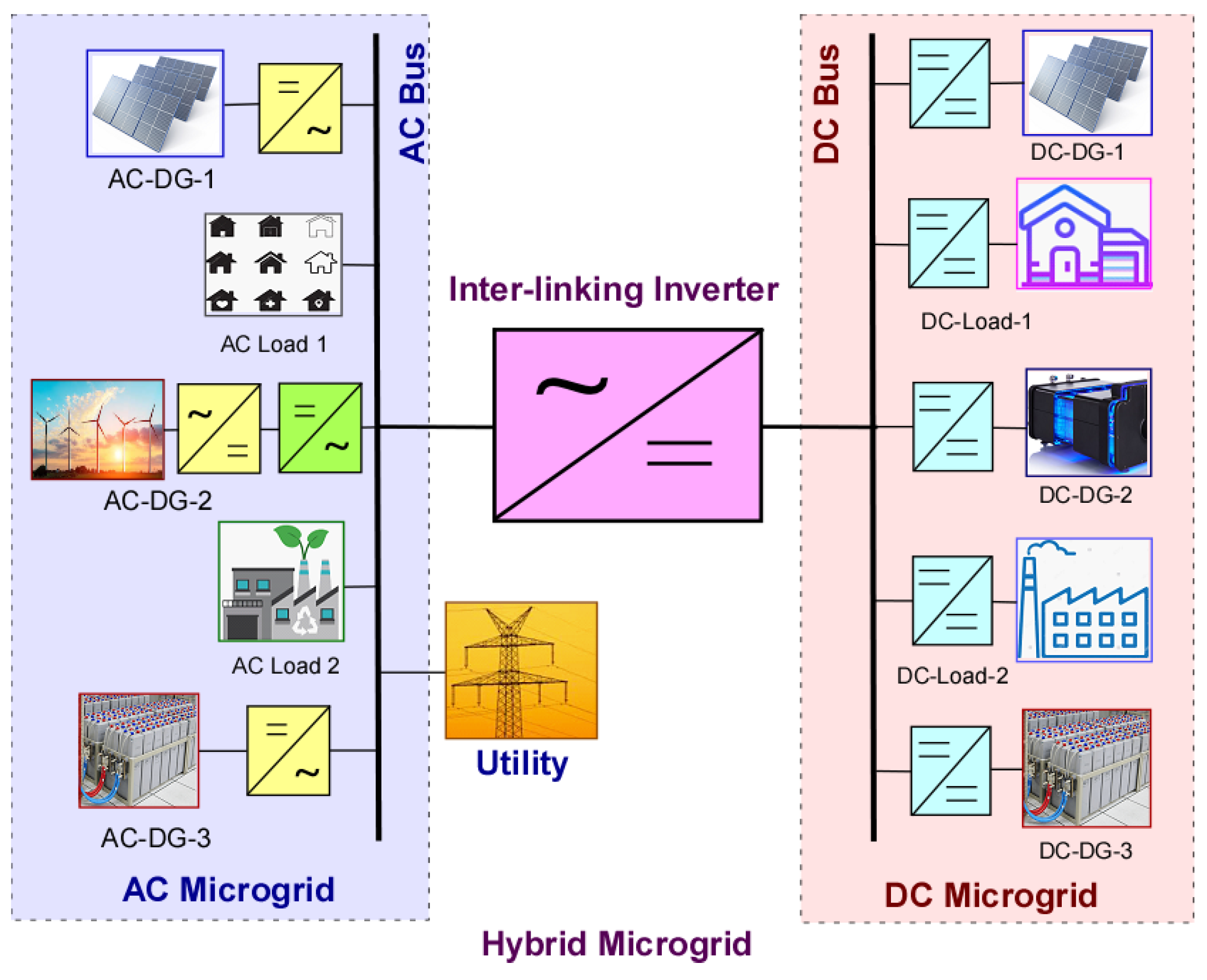Figure 2 displays one possible layout of a hybrid MG.

The hybrid MG provides a comprehensive solution to common issues like the suitability of sources and loads. It can integrate both DC and AC types of energy source and customer loads with the minimal (or zero) conversion stages. As shown in Figure 2, the interlinking inverter facilitates the power flow between the DC and AC MG and the main utility via the appropriate controllers. Thus, a hybrid MG’s autonomous operational capability is significantly higher than only DC- or AC-MG.

The MG’s control is either centralized or decentralized. Centralized control systems have the following advantages: (1) the main objectives are identified and realized; (2) they can offer global optimal decisions/solutions; (3) their synchronization to the main utility is relatively easy, and they can efficiently be operated online. On the other hand, decentralized control systems have the advantages: (1) they are appropriate for quickly changing infrastructures; (2) they can be easily expanded due to high capabilities of plug and play operation; (3) their reliability is high; (4) their communication and computational cost are relatively low [11,12]. Both centralized and decentralized controllers have been realized by many control algorithms such as H∞ [13], LQR [14], sliding mode [15], model-predictive control [16] and artificial intelligence techniques including fuzzy logic [5,17], neural networks [6], and genetic algorithms [18].

Remark 1.

It should be emphasized that [14] solves the problem of severe transients that occur during the transition between the connected and islanded modes of microgrids (which affect the voltage and frequency responses). The seamless transition is achieved by the linear quadratic regulators LQR with a simple pole placement method to select the weighting matrices Q and R. The bumpless transition is not considered in the present manuscript. The adaptive sliding control given in [15] achieves fast bus voltage tracking without additional sensors in addition to system scalability and maintaining the plug-and-play operation of the Distribution Generation units (DGs). By using the proposed method [15] to estimate the uncertainty and external disturbance, the system parameters and switching function can be adjusted in time to weaken the chattering. However, the control of [15] is non-linear, has some chattering, and is applied to only DC microgrids. The model-predictive control [16] is a time-varying tracker and requires significant computational time. The methods [5,6,18] also require extensive training and computational burdens.

Furthermore, decentralized control techniques manage, organize, and control an efficient short alteration from grid-connected mode to islanded mode [19]. It introduces and allows recent interlinking converter circuits to be used as quasi-Z-source converters [19]. The interlinking converter could be connected in series or parallel to enhance the hybrid MGs’ power quality. The series interlinking converter is used to improve the hybrid MGs, and the parallel voltage quality interlinking converter compensates for the harmonic voltage generated by the non-linear loads. In [20], a new circuit combination is anticipated for the interlinking converter to improve power quality indices. The interlinking converter is divided into two parts: parallel and series interlinking converter.

This paper introduces a control algorithm using invariant ellipsoids. The presented control technique avoids the complexity of selecting the weights of H∞ and the chattering issues of the sliding mode control. Moreover, it handles the parameter’s uncertainties and loads variations effectively. The contribution of the paper is:

(1)

A novel theorem, based on the linear matrix inequalities, is introduced to guarantee the optimal trackers’ solvability, in which the outputs follow the desired inputs and achieve external disturbance rejection.

(2)

A new simple controller is designed based on the invariant sets (approximated and bounded by invariant ellipsoids) is introduced. The proposed controller is fast, with a very low overshoot, and there is no chattering, unlike the sliding mode approach. It is also robust against load changes and system parameters uncertainties.

(3)

The need to add a feedforward path (to enhance the DGs’ controllers’ performance) is eliminated [21].

The paper is structured as follows. Section 2 presents the model of the investigated hybrid MG and the statement of the research problem. In Section 3, the control design is presented and described in detail. The results are displayed in Section 4. Finally, the conclusions are presented in Section 5.

Facts

Fact1:

$M\Delta \left(t\right)N+\ast <ϵM{M}^{\prime }+{ϵ}^{-1}{N}^{\prime }N$

The time-varying uncertainty ∆(t) can be removed using this fact

Fact 2 (Schur complements)

For a matrix M composed of

$M=\left[\begin{array}{cc}{M}_1& M_3\\ \ast & M_2\end{array}\right]$

where $M_1=M_{1 }^{\prime },M_2=M_2^{\prime }>0$ implies that M > 0 if and only if

$M_1-M_3{M}_2^{-1}{M}_3^{\prime }>0$

The last nonlinear matrix inequality can be linearized using this fact.

2. Model of the Hybrid Microgrid (MG) and Problem Statement

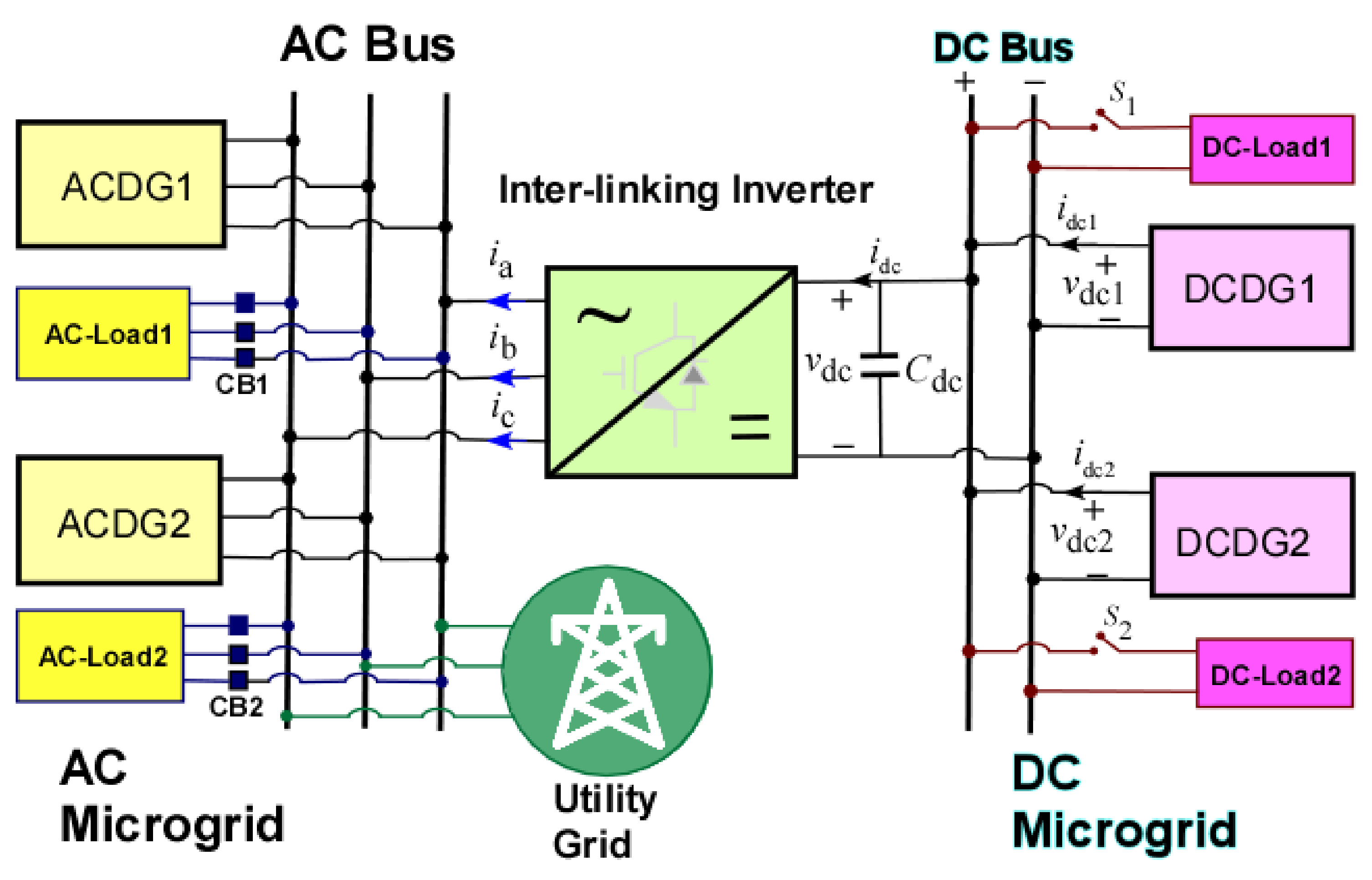
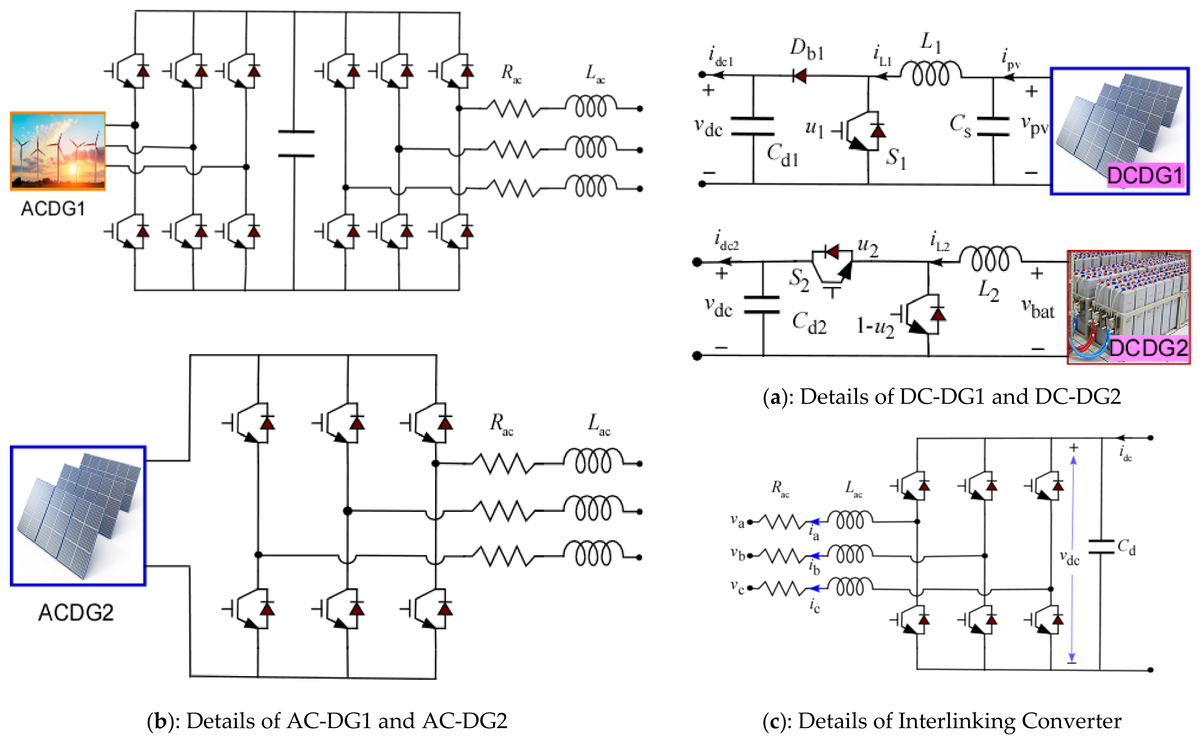
The model used in this paper is adapted from reference [19]. The studied hybrid MG consists of two DC sources, DC-DG1 and DC-DG2, as displayed in Figure 3. There are two AC sources, AC-DG1 and AC-DG2, and an inter-linking inverter. Details of the sources and inverters are depicted in Figure 4. DC-DG1 is a Photovoltaic (PV) system driven by a boost converter, as illustrated in Figure 4a. DC-DG2 is a Lithium-ion battery operated by a two-quadrant buck-boost converter. The AC-DG1 and AC-DG2 are PV and wind-turbine systems, respectively. They are controlled by three-phase voltage source converters, as shown in Figure 4b. Also, the inter-linking inverter is realized by a voltage source converter (Figure 4c). AC sources and the inter-linking converter are linked via Resistor-Inductor (RL) series filters. Referring to Figure 5, the AC side can be described by Equation (1).

$$\begin{array}{c}{L}_{\mathrm{ac}}\frac{d}{dt}{i}_{\mathrm{a}}=-R_{\mathrm{ac}}{i}_{\mathrm{a}}-v_{\mathrm{a}}+u_{\mathrm{a}}{v}_{\mathrm{dc}}\\ L_{\mathrm{ac}}\frac{d}{dt}{i}_{\mathrm{b}}=-R_{\mathrm{ac}}{i}_{\mathrm{b}}-v_{\mathrm{b}}+u_{\mathrm{b}}{v}_{\mathrm{dc}}\\ L_{\mathrm{ac}}\frac{d}{dt}{i}_{\mathrm{c}}=-R_{\mathrm{ac}}{i}_{\mathrm{c}}-v_{\mathrm{c}}+u_{\mathrm{c}}{v}_{\mathrm{dc}}\end{array}$$

(1)

where u_a, u_b, and u_c are the modulation indices for three-phase a, b, and c, respectively. Transforming (1) to the dq-reference frame yields Equations (2) and (3).

$$L_{\mathrm{ac}}\frac{d}{dt}{i}_{\mathrm{d}}=-R_{\mathrm{ac}}{i}_{\mathrm{d}}+\omega L_{\mathrm{ac}}{i}_{\mathrm{q}}-v_{\mathrm{d}}+u_{\mathrm{d}}{v}_{\mathrm{dc}}$$

(2)

$$L_{\mathrm{ac}}\frac{d}{dt}{i}_{\mathrm{q}}=-\omega L_{\mathrm{ac}}{i}_{\mathrm{d}}-R_{\mathrm{ac}}{i}_{\mathrm{q}}-v_{\mathrm{q}}+u_{\mathrm{q}}{v}_{\mathrm{dc}}$$

(3)

u_d and u_q, are d and the q-components of the modulation index of the inter-linking inverter, respectively. For the DC-DG1 and DC-DG2 sources, the following equations apply.

$$C_{\mathrm{s}}\frac{d}{dt}{v}_{\mathrm{pv}}=-i_{\mathrm{L}1}+i_{\mathrm{pv}}$$

(4)

$$L_1\frac{d}{dt}{i}_{\mathrm{L}1}=-v_{\mathrm{dc}}\left(1-u_1\right) + v_{\mathrm{pv}}$$

(5)

$$L_2\frac{d}{dt}{i}_{\mathrm{L}2}=-u_2{v}_{\mathrm{dc}}+v_{\mathrm{bat}}$$

(6)

u₁ and u₂, are the switching functions of DC-DG1 and DC-DG2, defined as follows.

$$u_1=\left\{\begin{array}{cc}1& S_1 \mathrm{is} \mathrm{on}\\ 0& S_1 \mathrm{is} \mathrm{off}\end{array}\right. \mathrm{and} u_2=\left\{\begin{array}{cc}1& S_2 \mathrm{is} \mathrm{on}\\ 0& S_2 \mathrm{is} \mathrm{off}\end{array}\right.$$

The DC-link voltage changes according to the difference between the ac-side powers (currents) and the dc-side powers (currents). Looking from DC-DG1, the v_dc state is expressed in Equation (7).

$$C_{\mathrm{d}1}\frac{d}{dt}{v}_{\mathrm{dc}}=i_{\mathrm{L}1}-u_1{i}_{\mathrm{L}1}-i_{\mathrm{dc}1}$$

(7)

Looking from the DC-DG2 side, the v_dc state is given in Equation (8).

$$C_{\mathrm{d}2}\frac{d}{dt}{v}_{\mathrm{dc}}=u_2{i}_{\mathrm{L}2}-i_{\mathrm{dc}2}$$

(8)

Looking from the AC side, the v_dc state is represented as in Equation (9).

$$C_{\mathrm{dc}}\frac{d}{dt}{v}_{\mathrm{dc}}=-u_{\mathrm{d}}{i}_{\mathrm{d}}-u_{\mathrm{q}}{i}_{\mathrm{q}}-i_{\mathrm{dc}}$$

(9)

Choosing C_d1 and C_d2 to be equal to C_dc and adding Equations (7)–(9) yields:

$$3C_{\mathrm{dc}}\frac{d}{dt}{v}_{\mathrm{dc}}=i_{\mathrm{L}1}\left(1-u_1\right) + u_2{i}_{\mathrm{L}2}-u_{\mathrm{d}}{i}_{\mathrm{d}}-u_{\mathrm{q}}{i}_{\mathrm{q}} - \left(i_{\mathrm{dc}}+i_{\mathrm{dc}1}+i_{\mathrm{dc}2}\right)$$

(10)

Equations (2)–(6) and (10) provide the hybrid MG’s model, with the states.

$$x={\left[\begin{array}{cccccc}{i}_{\mathrm{d}}& i_{\mathrm{q}}& v_{\mathrm{pv}}& i_{\mathrm{L}1}& i_{\mathrm{L}2}& v_{\mathrm{dc}}\end{array}\right]}^{\prime }$$

The model is nonlinear due to the product of the switching signals and their associated variables. To design the controller, this model should be linearized around an operating point. Here, the operating point is assumed as the voltages and currents’ nominal values. Then a perturbation is allowed around such an operating point. For instance, i_d is considered as: $i_{\mathrm{d}}=I_{\mathrm{d}}+\Delta i_{\mathrm{d}}$. I_d is the i_d’s value at the operating point (a quiescent value), and Δi_d is the perturbation.

Linearized Model

Substituting each state by its sum of a quiescent value and a perturbation in the Equations from (2) to (6), and (10), and neglecting the 2nd order terms, we get:

$$\begin{array}{c}\dot{\Delta i_{\mathrm{d}}}=\frac{\left(-R_{\mathrm{ac}}\Delta i_{\mathrm{d}}+\omega L_{\mathrm{ac}}\Delta i_{\mathrm{q}}-\Delta v_{\mathrm{d}}+U_{\mathrm{d}}\Delta v_{\mathrm{dc}}+V_{\mathrm{dc}}\Delta u_{\mathrm{d}}\right)}{L_{\mathrm{ac}}}\hfill \\ \dot{\Delta i_{\mathrm{q}}}=\frac{\left(-\omega L_{\mathrm{ac}}\Delta i_{\mathrm{d}}-R_{\mathrm{ac}}\Delta i_{\mathrm{q}}-\Delta v_{\mathrm{q}}+U_{\mathrm{q}}\Delta v_{\mathrm{dc}}+V_{\mathrm{dc}}\Delta u_{\mathrm{q}}\right)}{L_{\mathrm{ac}}}\hfill \\ \dot{\Delta v_{\mathrm{pv}}}=\frac{\left(-\Delta i_{\mathrm{L}1}+\Delta i_{\mathrm{pv}}\right)}{C_{\mathrm{s}}}\hfill \\ \dot{\Delta i_{\mathrm{L}1}}=\frac{\left(-\Delta v_{\mathrm{dc}}\left(1-U_1\right)+v_{\mathrm{dc}}\Delta u_1+\Delta v_{\mathrm{pv}}\right)}{L_1}\hfill \\ \dot{\Delta i_{\mathrm{L}1}}=\frac{\left(-U_2\Delta v_{\mathrm{dc}}-V_{\mathrm{dc}}\Delta u_2+v_{\mathrm{bat}}\right)}{L_2}\hfill \\ \dot{\Delta v_{\mathrm{dc}}}=\left(\begin{array}{c}\left(1-U_1\right)\Delta i_{\mathrm{L}1}+U_2\Delta i_{\mathrm{L}2}-I_{\mathrm{L}1}\Delta u_1+I_{\mathrm{L}2}\Delta u_2-U_{\mathrm{d}}\Delta i_{\mathrm{d}}-I_{\mathrm{d}}\Delta u_{\mathrm{d}}\\ -U_{\mathrm{q}}\Delta i_{\mathrm{q}}-I_{\mathrm{q}}\Delta u_{\mathrm{q}}-\frac{\left(\Delta i_{\mathrm{dc}}+\Delta i_{\mathrm{dc}1}+\Delta i_{\mathrm{dc}2}\right)}{\left(3C_{\mathrm{dc}}\right)}\end{array}\right)\hfill \end{array}$$

(11)

where $\dot{\Delta x}$ denotes the first derivative of x, and capital letters designate quiescent values. Thus, in state-space form, the model in Equation (11) is represented as in Equation (12).

$$\begin{array}{c}\dot{\Delta \mathrm{x}}=\mathrm{A}\Delta \mathrm{x}+\mathrm{B}\Delta \mathrm{u}+\mathrm{Dw}\hfill \\ \Delta \mathrm{y}=\mathrm{C}\Delta \mathrm{x}\hfill \\ \Delta \mathrm{x}={\left[\begin{array}{cccccc}\Delta i_{\mathrm{d}}& \Delta i_{\mathrm{q}}& \Delta v_{\mathrm{pv}}& \Delta i_{\mathrm{L}1}& \Delta i_{\mathrm{L}2}& \Delta v_{\mathrm{dc}}\end{array}\right]}^{\prime }\hfill \\ \Delta \mathrm{u}={\left[\begin{array}{cccc}\Delta u_{\mathrm{d}}& \Delta u_{\mathrm{q}}& \Delta u_1& \Delta u_2\end{array}\right]}^{\prime }\hfill \\ \mathrm{w}={\left[\begin{array}{ccccccc}\Delta v_{\mathrm{d}}& \Delta v_{\mathrm{q}}& \Delta i_{\mathrm{pv}}& \Delta v_{\mathrm{bat}}& \Delta i_{\mathrm{dc}}& \Delta i_{\mathrm{dc}1}& \Delta i_{\mathrm{dc}2}\end{array}\right]}^{\prime }\hfill \\ \Delta \mathrm{y}={\left[\begin{array}{cccc}\Delta i_{\mathrm{d}}& \Delta i_{\mathrm{q}}& \Delta v_{\mathrm{pv}}& \Delta v_{\mathrm{dc}}\end{array}\right]}^{\prime }\hfill \end{array}$$

(12)

where $\mathrm{x}\in {ℝ}^n$, $\mathrm{u}\in {ℝ}^p$, $\mathrm{y}\in {ℝ}^l$, and $\mathrm{w}\in {ℝ}^m$ are the state, control, output for feedback, and external disturbance vectors, respectively. Also,

$$\mathrm{A}= \left[\begin{array}{cccccc}-\frac{R_{\mathrm{ac}}}{L_{\mathrm{ac}}}& \omega & 0& 0& 0& \frac{U_{\mathrm{d}}}{L_{\mathrm{ac}}}\\ -\omega & -\frac{R_{\mathrm{ac}}}{L_{\mathrm{ac}}}& 0& 0& 0& \frac{U_{\mathrm{q}}}{L_{\mathrm{ac}}}\\ 0& 0& 0& -\frac{1}{C_{\mathrm{s}}}& 0& 0\\ 0& 0& \frac{1}{L_1}& 0& 0& -\frac{\left(1-U_1\right)}{L_1}\\ 0& 0& 0& 0& 0& -\frac{U_2}{L_2}\\ -\frac{U_{\mathrm{d}}}{3 C_{\mathrm{d}}}& -\frac{U_{\mathrm{q}}}{3 C_{\mathrm{d}}}& 0& \frac{1-U_1}{3 C_{\mathrm{d}}}& \frac{U_2}{3 C_{\mathrm{d}}}& 0\end{array}\right]$$

$$\mathrm{B}= \left[\begin{array}{cccc}\frac{V_{\mathrm{dc}}}{L_{\mathrm{ac}}}& 0& 0& 0\\ 0& \frac{V_{\mathrm{dc}}}{L_{\mathrm{ac}}}& 0& 0\\ 0& 0& 0& 0\\ 0& 0& \frac{V_{\mathrm{dc}}}{L_1}& 0\\ 0& 0& 0& -\frac{V_{\mathrm{dc}}}{L_2}\\ -\frac{I_{\mathrm{d}}}{3 C_{\mathrm{dc}}}& -\frac{I_{\mathrm{q}}}{3 C_{\mathrm{dc}}}& -\frac{I_{\mathrm{L}1}}{3 C_{\mathrm{dc}}}& \frac{I_{\mathrm{L}2}}{3 C_{\mathrm{dc}}}\end{array}\right]$$

$$\mathrm{D}=\left[\begin{array}{ccccccc}-\frac{1}{L_{\mathrm{ac}}}& 0& 0& 0& 0& 0& 0\\ 0& -\frac{1}{L_{\mathrm{ac}}}& 0& 0& 0& 0& 0\\ 0& 0& \frac{1}{C_{\mathrm{s}}}& 0& 0& 0& 0\\ 0& 0& 0& 0& 0& 0& 0\\ 0& 0& 0& \frac{1}{L_2}& 0& 0& 0\\ 0& 0& 0& 0& -\frac{1}{3C_{\mathrm{dc}}}& -\frac{1}{3C_{\mathrm{dc}}}& -\frac{1}{3C_{\mathrm{dc}}}\end{array}\right]$$

$$\mathrm{C} =\left[\begin{array}{cccccc}1& 0& 0& 0& 0& 0\\ 0& 1& 0& 0& 0& 0\\ 0& 0& 1& 0& 0& 0\\ 0& 0& 0& 0& 0& 1\end{array}\right]$$

To find the operating point, all the derivatives in equations from Equations (2)–(6) and (10) are set to zero. Then, by substituting all the variables by their values, a function of nine unknowns is formed as in Equation (13). Here is an example to illustrate the steps of obtaining Equation (13). Going back to Equation (2).

$$L_{\mathrm{ac}}\frac{d}{dt}{i}_{\mathrm{d}}=-R_{\mathrm{ac}}{i}_{\mathrm{d}}+\omega L_{\mathrm{ac}}{i}_{\mathrm{q}}-v_{\mathrm{d}}+u_{\mathrm{d}}{v}_{\mathrm{dc}}$$

Setting the derivative term to zero gives.

$$0=-R_{\mathrm{ac}}{i}_{\mathrm{d}}+\omega L_{\mathrm{ac}}{i}_{\mathrm{q}}-v_{\mathrm{d}}+u_{\mathrm{d}}{v}_{\mathrm{dc}}$$

Then i_d → I_d, i_q → I_q, v_d → V_d, u_d → U_d, and v_dc → V_dc, yield: −R_ac I_d + ωLI_q − V_d + U_dV_dc = 0. This is the first row in Equation (13).

$$\mathrm{f}\left(\mathrm{x}\right) =\left[\begin{array}{c}-R_{\mathrm{ac}}{I}_{\mathrm{d}}+\omega L{I}_{\mathrm{q}}-V_{\mathrm{d}}+U_{\mathrm{d}}{V}_{\mathrm{dc}}\\ -R_{\mathrm{ac}}{I}_{\mathrm{q}}-\omega L{I}_{\mathrm{d}}-V_{\mathrm{d}}+U_{\mathrm{q}}{V}_{\mathrm{dc}}\\ -I_{\mathrm{L}1}+I_{\mathrm{pv}}\\ -V_{\mathrm{dc}}\left(1-U_1\right)+V_{\mathrm{pv}}\\ -U_2{V}_{\mathrm{dc}}+V_{\mathrm{bat}}\\ I_{\mathrm{L}1}-U_{\mathrm{d}}{I}_{\mathrm{d}}-U_{\mathrm{q}}{I}_{\mathrm{q}}-U_1{I}_{\mathrm{L}1}+U_2{I}_{\mathrm{L}2}+I_{\mathrm{dc}}+I_{\mathrm{dc}1}+I_{\mathrm{dc}2}\end{array}\right]=0$$

(13)

The knowns are I_q, I_dc, U_d, U_q, U₁, U₂, I_L1, I_L2, and V_dc. The parameters in (13) are listed in

Table 1. Hybrid MG parameters [19].

Parameter	Symbol	Value	Unit
AC-side Resistance	Rac	0.30	Ω
AC-side Inductance	Lac	3.0	mH
Input Capacitance of DC-DG1	Cs	110.0	μF
DC-side Capacitance of DC-DG1	Cdc	60.0	μF
Inductance of DC-DG1	L1	8.0	mH
Inductance of DC-DG2	L2	8.0	mH

and

Table 2. Hybrid MG nominal values [19].

Variable	Symbol	Value	Unit
Fundamental Frequency	ω	100π	rad/s
AC-side Voltage	Va	220.0	V
DC voltage of DC-DG1 and DC-DG2	Vpv,Vbat	600.0	V
DC-link Voltage	Vdc	700.0	V
Battery Capacity, DC-DG2	Cbat	22.0	Ah
AC-side Active Power	Pac	12.0	kW
AC-side Reactive Power	Qac	10.0	kVAr
MPPT PV power	Ppv	4.50	kW
Switching Frequency	fsw	10.0	kHz

, with their used values.

In Equation (13), it is noticed that the number of equations is less than the number of unknowns. Thus, the damped least square (Levenberg–Marquardt algorithm, via the function fsolve in Matlab) is used to solve it with an initial guess:

$${\mathrm{x}}^{\prime } = [0, 18, 1, 1, 1, 1, 7.5, 7.5, 700].$$

Table 3. Operating point: solution of Equation (13).

Variable	Value
Iq	−6.7239 A
Idc	5.3584 A
Ud	0.3311
Uq	0.0216
U1	0.1429
U2	0.8571
IL1	6.0775 A
IL2	19.3244 A
Vdc	700.0219 V

shows the solution results for the nine unknowns in (13), noting that the values of U₁, U₂, U_d, U_q are dimensionless.

After getting the operation point, these values are substituted in Equation (12) to obtain the linearized hybrid MG model.

The problem can be stated as follows. It is required to design a controller based on the linearized model for the studied hybrid MG. The controller has to be robust against parameter variations modelled as norm-bounded uncertainty. The proposed controller is to be tested on the original non-linear model of the hybrid MG.

3. Controller Design

3.1. The Invariant (or Attractive) Ellipsoid Set

The attractive (or invariant) ellipsoid design has recently been developed in robust control of linear and non-linear systems [22]. Moreover, the ellipsoidal design is successfully applied in many applications, e.g., automatic generation control [23], piezoelectric actuators [24], car active suspension [25], islanded AC microgrids [26,27].

The basic idea of the ellipsoidal design is as follows. For an initial state vector outside the ellipsoid, the state trajectory must be attracted to a small ellipsoidal region, including the origin (attracting ellipsoid). When the trajectory reaches the ellipsoid, it will not leave it (invariant ellipsoid) [28]. The linear time-invariant (LTI) system (12) is rewritten, removing the ∆ for simplicity, as follows:

$$\begin{array}{cc}\dot{\mathrm{x}}=\mathrm{Ax}+\mathrm{Bu}+\mathrm{Dw},\hfill & \mathrm{y}=\mathrm{Cx},\hfill \\ \mathrm{z}={\mathrm{C}}_{\mathrm{z}}\mathrm{x}+{\mathrm{B}}_2\mathrm{u}\hfill \end{array}$$

(14)

The vector $\mathrm{z}$ is the output to be optimized (the effect of disturbance w on z must be minimized). The term ${\mathrm{B}}_2\mathrm{u}$ is added to z to avoid obtaining controller with large gains, challenging to implement in practice. It is assumed that ${\mathrm{C}}_{\mathrm{z}}=\mathrm{C}.$

3.2. Design Procedure

There are two control problems: (1) regulator (for constant reference), (2) tracking (for time-varying reference). The output must track the desired time-varying reference with zero steady-state error in the hybrid microgrid control. Therefore, an integrator must be inserted, as will be seen later.

3.3. Regulator Ellipsoidal Design

The LTI system (14) assumes that the pair (A, B) is controllable, and the pair (A, C) is observable under a bounded external disturbance $\mathrm{Dw}$. The disturbance is subject to the following constraint:

$$\Vert \mathrm{w}\left(t\right)\Vert \le 1, t\ge 0$$

(15)

Note that the constraint in Equation (15) can be realized by scaling the matrix D.

Consider an ellipsoid E with origin as the centre given by the following equation:

$$E={\mathrm{x}}^{\prime }{\mathrm{P}}^{-1}\mathrm{x}\le 1, \mathrm{P}>0$$

(16)

The ellipsoid also represents a Lyapunov function $\mathrm{V}\left(\mathrm{x}\right)={\mathrm{x}}^{\prime }{\mathrm{P}}^{-1}\mathrm{x}$, if the initial state vector $\mathrm{x}\left(0\right)$ lies outside the ellipsoid, V does not increase outside this ellipsoid. In other words, $\dot{\mathrm{V}}\left(\mathrm{x}\right) \le 0 \mathrm{for} \mathrm{all} \mathrm{x}\left(t\right) \mathrm{subject} \mathrm{to} \mathrm{V}\left(\mathrm{x}\right) \ge 1,$ i.e., the state trajectory $\mathrm{x}\left(t\right)$ is attracted to the ellipsoid. When the trajectory of $\mathrm{x}\left(t\right)$ reaches the ellipsoid, it will not leave it for the future time (time-invariant). The ellipsoid is thus attractive and invariant.

Remark 2.

For an initial state vector x(0) starting outside the ellipsoid $\mathrm{V}\left(\mathrm{x}\right)={\mathrm{x}}^{\prime }{\mathrm{P}}^{-1}\mathrm{x}$, the proposed design is based on attracting the state trajectories to the ellipsoid by requiring $\dot{\mathrm{V}}\left(\mathrm{x}\right) \le 0 \mathit{for} \mathit{all} \mathrm{x}\left(\mathrm{t}\right) \mathit{subject} \mathit{to} \mathrm{V}\left(\mathrm{x}\right) \ge 1$. Once the trajectories x(t) arrive at the ellipsoid, it will not leave it for the future time. This constraint and the disturbance norm constraint Equation (15) are cast in one matrix inequality Equation (17) using Schur complements, Fact 2.

It is shown in [28] that E is invariant (and attracting) for the system (14) if and only if there exists a scalar $\alpha >0, \mathrm{and} \mathrm{a} \mathrm{symmetric} \mathrm{matrix} \mathrm{P}>0$ solutions to the following non-linear matrix equation:

$$\left[\begin{array}{cc}\left(\mathrm{AP}+\mathrm{BY}+\ast \right) + \alpha \mathrm{P}& \mathrm{D}\\ \ast & -\alpha \mathrm{I}\end{array}\right] \le 0$$

(17)

where $\mathrm{Y}=\mathrm{KP}.$ The source of non-linearity is the product term $\alpha \mathrm{P}.$ The disturbance effect on the trajectory x can be rejected by minimizing the ellipsoid volume as follows:

$$minimize tr\left(\mathrm{P}\right)$$

(18)

where tr(P) is the trace function (the sum of the diagonal elements of P), selected due to its linearity, which provides a semidefinite program (SDP) that can be easily solved by Matlab convex optimization, as will be seen later.

To find the effect of the disturbance on the output to optimize $\mathrm{z}= \left(\mathrm{C}+{\mathrm{B}}_2\mathrm{K}\right)\mathrm{x}$, the ellipsoid in Equation (16) is replaced by:

$$E_{\mathrm{z}}={\mathrm{z}}^{\prime }{(\left(\mathrm{C}+{\mathrm{B}}_2\mathrm{K}\right)\mathrm{P}{\left(\mathrm{C}+{\mathrm{B}}_2\mathrm{K}\right)}^{\prime })}^{-1}\mathrm{z}\le 1$$

(19)

The effect of the disturbance on z is minimized by:

$$minimize tr\left[\left(\mathrm{C}+{\mathrm{B}}_2\mathrm{K}\right)\mathrm{P}{\left(\mathrm{C}+{\mathrm{B}}_2\mathrm{K}\right)}^{\prime }\right]$$

(20)

The proposed controller, which reduces (or rejects) the disturbance effect on the output z, is obtained by the following theorem.

Theorem 1

[28]. Consider the LTI system (14), subject to the disturbance described in (15). Then, a state feedback regulator can stabilize the system:

$$\mathrm{u}=\mathrm{Kx}$$

(21)

is equivalent to:

$$minimize tr\left[{\mathrm{CPC}}^{\prime } + \left({\mathrm{CY}}^{\prime }{\mathrm{B}}_2^{\prime }+\ast \right) + {\mathrm{B}}_2{\mathrm{ZB}}_2^{\prime }\right]$$

(22)

subject to the constraints:

$$\begin{array}{c}\left[\begin{array}{cc}\left(\mathrm{AP}+\mathrm{BY}+\ast \right) + \alpha \mathrm{P}& \mathrm{D}\\ \ast & -\alpha \mathrm{I}\end{array}\right] \le 0,\alpha >0\hfill \\ \left[\begin{array}{c}\mathrm{Z} \mathrm{Y}\\ \ast \mathrm{P}\end{array}\right] \ge 0, \mathrm{P}>0\hfill \end{array}$$

(23)

where $\mathrm{Y}=\mathrm{K}\mathrm{P}$ and the minimization is carried out to the variables α, $\mathrm{P}={\mathrm{P}}^{\prime }\in {\mathbb{R}}^{\mathrm{n}\times \mathrm{n}},\mathrm{Y}\in {\mathbb{R}}^{\mathrm{p}\times \mathrm{n}}$ and $\mathrm{Z}={\mathrm{Z}}^{\prime }\in {\mathbb{R}}^{\mathrm{p}\times \mathrm{p}}$. Let $\mathrm{Y}=\mathrm{K}\mathrm{P}$. Then the regulator is given by the Equation (24).

$$\mathrm{K}={\mathrm{YP}}^{-1}$$

(24)

Fixing $\alpha$ in the nonlinear matrix Equation (23) results in an LMI. The objective function is iteratively minimized by fixing $\alpha$ for every iteration. Therefore SDP in one-dimensional convex optimization is obtained and easy to solve by the LMI toolbox.

3.4. Tracker Ellipsoidal Design

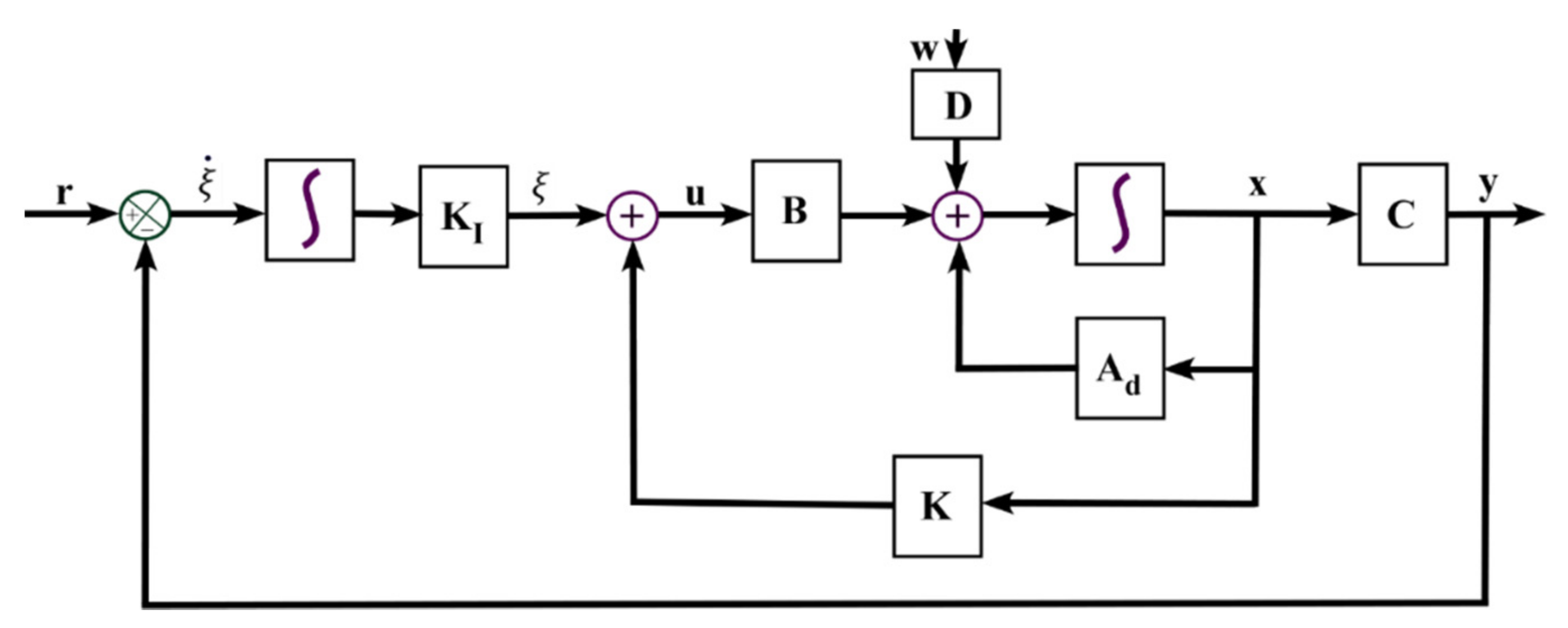
The above theorem can be generalized to the tracking problem by inserting an integral part between the plant’s error signal and the plant, as shown in Figure 5.

State feedback plus integral control is proposed in the form:

$$\mathrm{u}=\mathrm{K} \mathrm{x}+{\mathrm{K}}_{\mathrm{i}} \mathsf{\xi }=\left[\begin{array}{cc}\mathrm{K}& {\mathrm{K}}_{\mathrm{i}}\end{array}\right]\left[\begin{array}{c}\mathrm{x}\\ \mathsf{\xi }\end{array}\right] , \dot{\mathsf{\xi }}=\mathrm{r}-\mathrm{C} \mathrm{x}$$

(25)

Therefore, the augmented system is:

$$\left[\begin{array}{c}\dot{\mathrm{x}}\\ \dot{\mathsf{\xi }}\end{array}\right]=\left[\begin{array}{cc}\mathrm{A}& 0\\ -\mathrm{C}& 0\end{array}\right]\left[\begin{array}{c}\mathrm{x}\\ \mathsf{\xi }\end{array}\right]+\left[\begin{array}{c}\mathrm{B}\\ 0\end{array}\right]\mathrm{u}+\left[\begin{array}{c}\mathrm{D}\\ 0\end{array}\right]\mathrm{w}+\left[\begin{array}{c}0\\ \mathrm{I}\end{array}\right]\mathrm{r}, \mathrm{z}=\left[\begin{array}{cc}\mathrm{C}& 0\end{array}\right]\left[\begin{array}{c}\mathrm{x}\\ \mathsf{\xi }\end{array}\right]+{\mathrm{B}}_2\mathrm{u}$$

(26)

or

$$\left[\begin{array}{c}\dot{\mathrm{x}}\\ \dot{\mathsf{\xi }}\end{array}\right]= \widehat{\mathrm{A}}\left[\begin{array}{c}\mathrm{x}\\ \mathsf{\xi }\end{array}\right]+ \widehat{\mathrm{B}} \mathrm{u}+ \widehat{\mathrm{D}} \mathrm{w}+\left[\begin{array}{c}0\\ \mathrm{I}\end{array}\right]\mathrm{r},\mathrm{z}= \widehat{\mathrm{C}}\left[\begin{array}{c}\mathrm{x}\\ \mathsf{\xi }\end{array}\right]+{\mathrm{B}}_2\mathrm{u}$$

(27)

where the augmented matrices are:

$$\begin{array}{cc}\widehat{\mathrm{A}}=\left[\begin{array}{cc}\mathrm{A}& 0\\ -\mathrm{C}& 0\end{array}\right], \widehat{\mathrm{B}}=\left[\begin{array}{c}\mathrm{B}\\ 0\end{array}\right], \widehat{\mathrm{D}}=\left[\begin{array}{c}\mathrm{D}\\ 0\end{array}\right]& \widehat{\mathrm{C}}=\left[\begin{array}{c}\mathrm{C}\\ 0\end{array}\right]\end{array}$$

(28)

The design of regulators via the ellipsoidal sets, Theorem 1, can be generalized to the problem of the tracker’s design. The suggested controller must be robust against the parameters uncertainties and load variations of the hybrid MG. Thus, Equation (28) is adapted to:

$$\left[\begin{array}{c}\dot{\mathrm{x}}\\ \dot{\mathsf{\xi }}\end{array}\right]=\left( \widehat{\mathrm{A}}+\mathsf{\Delta }\widehat{\mathrm{A}}\right)\left[\begin{array}{c}x\\ \mathsf{\xi }\end{array}\right]+\left( \widehat{\mathrm{B}}+\Delta \widehat{\mathrm{B}}\right)\mathrm{u}+\left(\widehat{\mathrm{D}}+\mathsf{\Delta }\widehat{\mathrm{D}}\right)\mathrm{w}+\left[\begin{array}{c}0\\ \mathrm{I}\end{array}\right]\mathrm{r}, \mathrm{z}=\widehat{\mathrm{C}}\left[\begin{array}{c}x\\ \mathsf{\xi }\end{array}\right]+{\mathrm{B}}_2\mathrm{u}$$

(29)

where the following norm-bounded model represents the uncertainties:

$$\begin{array}{c}\Delta \widehat{\mathrm{A}} \le \mathrm{M}\Delta \left(\mathrm{t}\right)\mathrm{N}, \Vert \Delta \left(\mathrm{t}\right)\Vert \le 1; \Delta \widehat{\mathrm{B}} \le {\mathrm{M}}_{\mathrm{B}}{\Delta }_{\mathrm{B}}\left(\mathrm{t}\right){\mathrm{N}}_{\mathrm{B}}, \Vert {\Delta }_{\mathrm{B}}\left(\mathrm{t}\right)\Vert \le 1\hfill \\ \Delta \widehat{\mathrm{D}} \le {\mathrm{M}}_{\mathrm{D}}{\Delta }_{\mathrm{D}}\left(\mathrm{t}\right){\mathrm{N}}_{\mathrm{D}}, \Vert {\Delta }_{\mathrm{D}}\left(\mathrm{t}\right)\Vert \le 1\hfill \end{array}$$

(30)

The norm-bounded form can be obtained using the singular value decomposition (decomposing a matrix into the multiplication of three matrices). Finally, Theorem 2 is developed to determine the controller without any trial and error.

Theorem 2.

Assume that the system (29) is controllable $(\widehat{\mathrm{A}},\widehat{\mathrm{B}})$, and observable $(\widehat{\mathrm{A}},\widehat{\mathrm{C}})$, under L_∞-bounded exogenous disturbances. Then, the robust disturbance-rejection state feedback plus integral controller $\mathrm{u}=\left[\begin{array}{cc}\mathrm{K}& {\mathrm{K}}_i\end{array}\right]\left[\begin{array}{c}\mathrm{x}\\ \mathsf{\xi }\end{array}\right]$ is obtained by solving: $minimize tr\left[\widehat{\mathrm{C}}\widehat{\mathrm{P}}{\widehat{\mathrm{C}}}^{\prime }+\left(\widehat{\mathrm{C}}{\widehat{\mathrm{Y}}}^{\prime }{\mathrm{B}}_2^{\prime }+\ast \right)+{\mathrm{B}}_2\mathrm{Z}{\mathrm{B}}_2^{\prime }\right]$, subject to the following constraints:

$$\begin{array}{cc}\left[\begin{array}{ccccc}\mathsf{\phi }& \widehat{\mathrm{D}}& \widehat{\mathrm{P}}{\mathrm{N}}^{\prime }& 0& {\widehat{\mathrm{Y}}}^{\prime }{\mathrm{N}}_{\mathrm{B}}^{\prime }\\ \ast & -\alpha \mathrm{I}& 0& {\mathrm{N}}_{\mathrm{D}}^{\prime }& 0\\ \ast & \ast & -ϵ\mathrm{I}& 0& 0\\ \ast & \ast & \ast & -\rho \mathrm{I}& 0\\ \ast & \ast & \ast & \ast & -\pi \mathrm{I}\end{array}\right]\le 0,\hfill & \alpha ,ϵ,\rho ,\pi >0\hfill \\ \mathrm{Where} \mathsf{\phi }=\left( \widehat{\mathrm{A}} \widehat{\mathrm{P}}+ \widehat{\mathrm{B}}\widehat{\mathrm{Y}}+\ast \right) + \alpha \widehat{\mathrm{P}}+ϵ\mathrm{M}{\mathrm{M}}^{\prime }+{\rho \mathrm{M}}_{\mathrm{D}}{\mathrm{M}}_{\mathrm{D}}^{\prime }+{\mu \mathrm{M}}_{\mathrm{B}}{\mathrm{M}}_{\mathrm{B}}^{\prime }\hfill \\ \left[\begin{array}{cc}Z& \widehat{\mathrm{Y}}\\ \ast & \widehat{\mathrm{P}}\end{array}\right]\ge 0, \widehat{P}>0\hfill \end{array}$$

(31)

where$\widehat{\mathrm{Y}}=\widehat{\mathrm{K}}\widehat{\mathrm{P}},\widehat{\mathrm{K}}=\left[\begin{array}{cc}\mathrm{K}& {\mathrm{K}}_{\mathrm{i}}\end{array}\right]$. The minimization is carried out to the variables $\dots \epsilon ,\rho ,\mu , \mathrm{P}={\mathrm{P}}^{\prime }\in {\mathbb{R}}^{\left(\mathrm{n}+\mathrm{l}\right)·\left(\mathrm{n}+\mathrm{l}\right)}$, $\widehat{\mathrm{Y}}\in {\mathbb{R}}^{\mathrm{p}·\left(\mathrm{n}+\mathrm{l}\right)}$. Note that this theorem does not impose the matching condition $\left[\begin{array}{ccc}\Delta \widehat{\mathrm{A}}& \Delta \widehat{\mathrm{B}}& \Delta \widehat{\mathrm{D}}\end{array}\right]=\mathrm{M}\Delta \left(\mathrm{t}\right)\left[\begin{array}{ccc}\mathrm{N}& {\mathrm{N}}_{\mathrm{B}}& {\mathrm{N}}_{\mathrm{D}}\end{array}\right]$.

Proof. 

For the tracking problem, the matrices in (14) are replaced by the augmented system matrices. Thus, Equation (17) becomes:

$$\left[\begin{array}{cc}\left(\widehat{\mathrm{A}}\widehat{\mathrm{P}}+ \widehat{\mathrm{B}}\widehat{\mathrm{Y}} + \ast \right)+\alpha \widehat{\mathrm{P}}& \widehat{\mathrm{D}}\\ \ast & -\alpha \mathrm{I}\end{array}\right] \le 0,\alpha >0$$

(32)

To tackle the load variations in the hybrid MG, $\widehat{\mathrm{A}} \mathrm{is} \mathrm{substituted} \mathrm{by} \left(\widehat{\mathrm{A}}+ \mathsf{\Delta }\widehat{\mathrm{A}}\right), \widehat{\mathrm{B}} \mathrm{by} \left(\widehat{\mathrm{B}}+\Delta \widehat{\mathrm{B}}\right), \mathrm{and} \widehat{\mathrm{D}} \mathrm{by} \left(\widehat{\mathrm{D}}+\mathsf{\Delta }\widehat{\mathrm{D}}\right)$ in Equation (32), resulting in:

$$\left[\begin{array}{cc}\left(\left(\widehat{\mathrm{A}}+\Delta \widehat{\mathrm{A}}\right)\widehat{\mathrm{P}}+\left(\widehat{\mathrm{B}}+\Delta \widehat{\mathrm{B}}\right)\widehat{\mathrm{Y}}+\ast \right)+\alpha \widehat{\mathrm{P}}& \widehat{\mathrm{D}}+\Delta \widehat{\mathrm{D}}\\ \ast & -\alpha \mathrm{I}\end{array}\right]\le 0, \alpha >0$$

Substituting for the norm-bounded uncertainty Equation (30), one obtains:

$$\left[\begin{array}{cc}\left(\left(\widehat{\mathrm{A}}+\mathrm{M}\Delta \mathrm{N}\right)\widehat{\mathrm{P}}+\left(\widehat{\mathrm{B}}+{\mathrm{M}}_{\mathrm{B}}{\mathsf{\Delta }}_{\mathrm{B}}{\mathrm{N}}_{\mathrm{B}}\right)\widehat{\mathrm{Y}}+\ast \right)+\alpha \widehat{\mathrm{P}}& \widehat{\mathrm{D}}+{\mathrm{M}}_{\mathrm{D}}{\mathsf{\Delta }}_{\mathrm{D}}{\mathrm{N}}_{\mathrm{D}}\\ \ast & -\alpha \mathrm{I}\end{array}\right]\le 0, \alpha >0$$

Separating the uncertainty terms, we obtain:

$$\begin{array}{l}\left[\begin{array}{cc}\left(\widehat{\mathrm{A}}\widehat{\mathrm{P}}+ \widehat{\mathrm{B}}\widehat{\mathrm{Y}} + \ast \right)+\alpha \widehat{\mathrm{P}}& \widehat{\mathrm{D}}\\ \ast & -\alpha \mathrm{I}\end{array}\right]+\left(\left[\begin{array}{c}\mathrm{M}\\ 0\end{array}\right]\Delta \left[\begin{array}{cc}\mathrm{N}\widehat{\mathrm{P}}& 0\end{array}\right]+\ast \right)\\ +\left(\left[\begin{array}{c}{\mathrm{M}}_{\mathrm{B}}\\ 0\end{array}\right]{\Delta }_{\mathrm{B}}\left[\begin{array}{cc}{\mathrm{N}}_{\mathrm{B}}\widehat{\mathrm{Y}}& 0\end{array}\right]+\ast \right)+\left(\left[\begin{array}{c}{\mathrm{M}}_{\mathrm{D}}\\ 0\end{array}\right]{\Delta }_{\mathrm{D}}\left[\begin{array}{cc}0& {\mathrm{N}}_{\mathrm{D}}\widehat{\mathrm{Y}}\end{array}\right]+\ast \right)\le 0\end{array}$$

(33)

Using Fact 1 to eliminate ${\mathsf{\Delta }}_{\mathrm{A}}\left(t\right), {\mathsf{\Delta }}_{\mathrm{B}}\left(t\right), \mathrm{and} {\mathsf{\Delta }}_{\mathrm{D}}\left(t\right)$, (33) is fulfilled if the following matrix equation is satisfied:

$$\left[\begin{array}{cc}\left(\widehat{\mathrm{A}} \widehat{\mathrm{P}}+\widehat{\mathrm{B}}\widehat{\mathrm{Y}}+\ast \right)+\alpha \widehat{\mathrm{P}}& \widehat{\mathrm{D}}\\ \ast & -\alpha \mathrm{I}\end{array}\right]+ϵ\left[\begin{array}{c}\mathrm{M}\\ 0\end{array}\right]{\left[\begin{array}{c}\mathrm{M}\\ 0\end{array}\right]}^{\prime }+{ϵ}^{-1}\left[\begin{array}{c}\widehat{\mathrm{P}}{\mathrm{N}}^{\prime }\\ 0\end{array}\right]{\left[\begin{array}{c}\widehat{\mathrm{P}}{\mathrm{N}}^{\prime }\\ 0\end{array}\right]}^{\prime }$$

$$+\mu \left[\begin{array}{c}{\mathrm{M}}_{\mathrm{B}}\\ 0\end{array}\right]{\left[\begin{array}{c}{\mathrm{M}}_{\mathrm{B}}\\ 0\end{array}\right]}^{\prime }+{\mu }^{-1}\left[\begin{array}{c}{\widehat{\mathrm{Y}}}^{\prime }{\mathrm{N}}_{\mathrm{B}}^{\prime }\\ 0\end{array}\right]{\left[\begin{array}{c}{\widehat{\mathrm{Y}}}^{\prime }{\mathrm{N}}_{\mathrm{B}}^{\prime }\\ 0\end{array}\right]}^{\prime }+\rho \left[\begin{array}{c}{\mathrm{M}}_{\mathrm{D}}\\ 0\end{array}\right]{\left[\begin{array}{c}{\mathrm{M}}_{\mathrm{D}}\\ 0\end{array}\right]}^{\prime }+{\rho }^{-1}\left[\begin{array}{c}0\\ {\mathrm{N}}_{\mathrm{D}}^{\prime }\end{array}\right]{\left[\begin{array}{c}0\\ {\mathrm{N}}_{\mathrm{D}}^{\prime }\end{array}\right]}^{\prime }\le \begin{array}{cc}0,& \alpha ,ϵ,\rho ,\mu \end{array}>0$$

Using Fact 2, Theorem 2 is proved. □

3.5. Gain Matrices

Solving the above LMI (31) yields the following gain matrices of the proposed controller.

K =	[−905.75,	−0.0031213	0.45549	0.74613	−0.35706	1623.9
	−0.22601	−906.7	−0.21299	−0.22843	0.1109	−504.42
	116.63	1.3025	2819.2	97.073	−59.051	2.6869 × 105
	1096.1	2.2905	879.07	1178.7	−559.74	2.5753 × 106]

Ki =	[−116.8	127.98	121.12	37.791
	67.158	−306.96	−277.58	−188.36
	−242.35	985.24	341.2	−341.89
	35,952	15,082	−7324.5	15,313]

4. Simulation Results

The hybrid MG system shown in Figure 3 and Figure 4 was studied, tested, and implemented using Matlab/Simulink Power Library. The ellipsoid tracking control algorithm was assessed with two different sets of the MG parameters provided in

Table 4. Two different sets of MG parameters.

Parameter	First Set	Second Set
AC-side Resistance (Rac)	100%	115%
AC-side Inductance (Lac)	100%	90%
Input Capacitance of DC-DG1 (Cs)	100%	85%
DC-side Equivalent Capacitance of DC-DG1 (Cdc)	100%	110%
Inductance of DC-DG1 (L1)	100%	85%
Inductance of DC-DG2 (L2)	100%	85%

. Table 2 provides further specifications of the proposed MG.

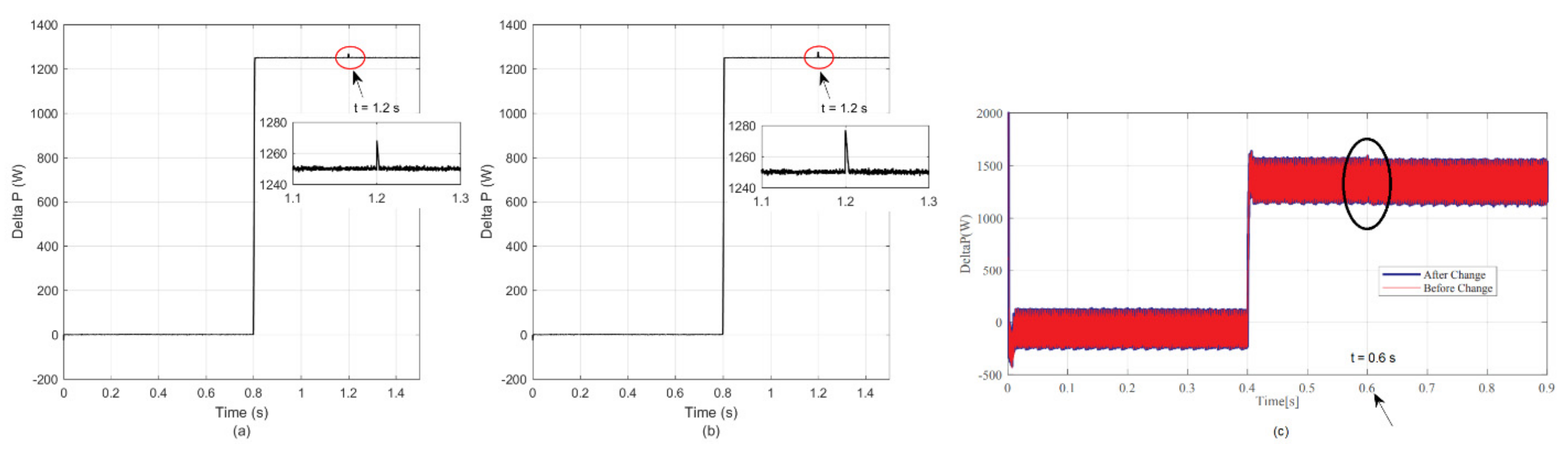
The DGs on the AC MG provide their local load demands. When the CB1 is closed, the load connected to the AC-DG1 (wind turbine system) is changed at t = 0.8 s, increased by 1.25 kW and 1.0 kVAR. Moreover, when the CB2 is closed, the load connected to AC-DG2 (PV inverter 2) is changed at t = 1.2 s, increased by 2.2 kW and 1.5 kVAR. Both cases will happen under two different sets of the MG parameters, as illustrated in Table 4. The proposed control technique was compared with the sliding mode controller used in [19]. The comparison between both techniques is shown in all figures from Figure 6, Figure 7, Figure 8, Figure 9 and Figure 10 and Figures 12–17.

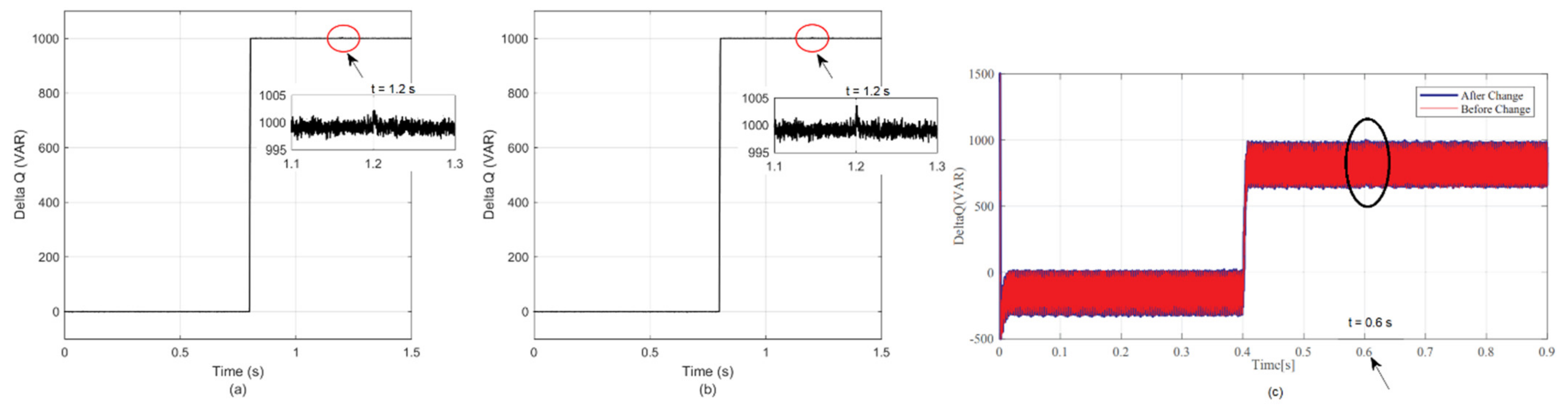
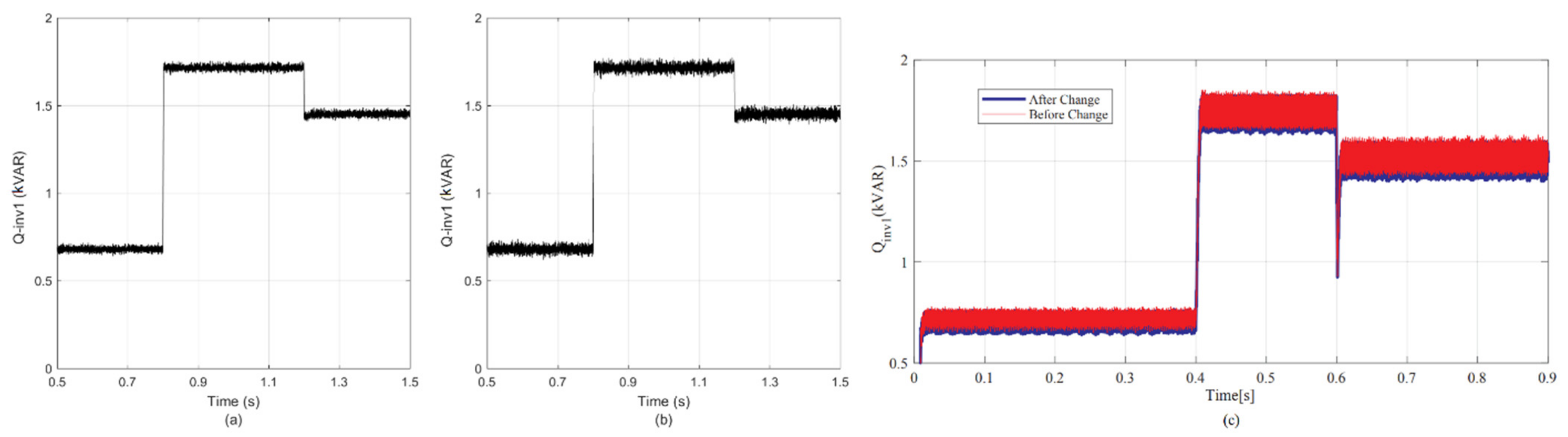
The changes of power (active and reactive) in the AC MG are given in Figure 6 and Figure 7. At t = 0.8 s, changes in active power (Delta P) are shown in Figure 6a and Figure 7a for the first and second parameters sets, respectively. The changes in reactive power (Delta Q) are displayed in Figure 6b and Figure 7b for the first and second parameter sets, respectively. Furthermore, Figure 6c and Figure 7c show the sliding mode technique [19] results for this case. The proposed technique is fast, with low spikes, and has no chattering compared to the sliding mode technique used in [19].

The transient and steady-state responses of the DC, AC-MG state variables, and power-sharing of the hybrid MG using the proposed technique is tested, verified, and compared to the sliding mode technique used in [19] in the following subsections.

4.1. Direct Current (DC) Side State Variables

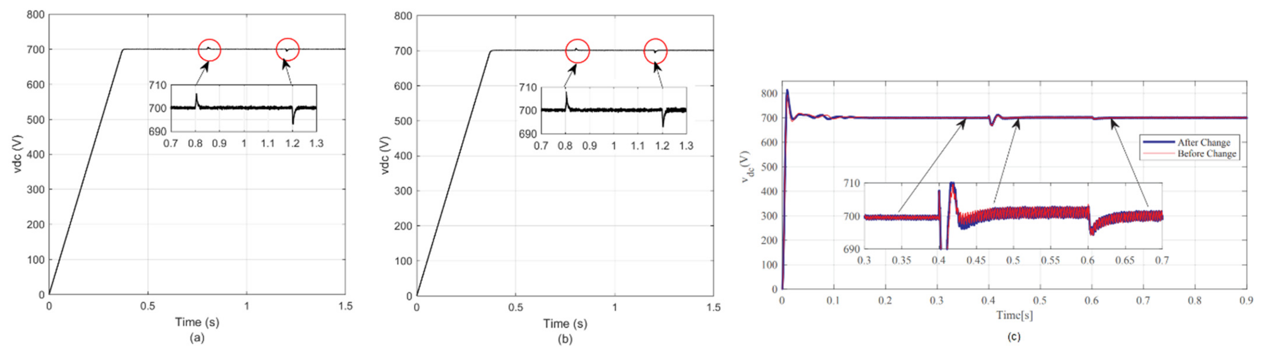
The DC-link voltage of the inter-linking converter is illustrated in Figure 8. In Figure 8a,b, the DC-link as a dc state variable is assessed with the two different sets of the MG parameters (Table 4). The DC-link voltage responses with these two sets of parameters and added loads in the AC side during t = 0.8 s and t = 1.2 s respond perfectly with a difference between the spikes rates that is too small. Therefore, v_dc with a stable steady-state and dynamic response is accomplished. Figure 8c shows the DC-link voltage response for the sliding mode control technique [19]. The comparison between both techniques shows that the DC-link voltage response’s proposed technique is a bit slower. Nonetheless, it rejects the load disturbance efficiently without the high chattering in the sliding-mode control technique [19].

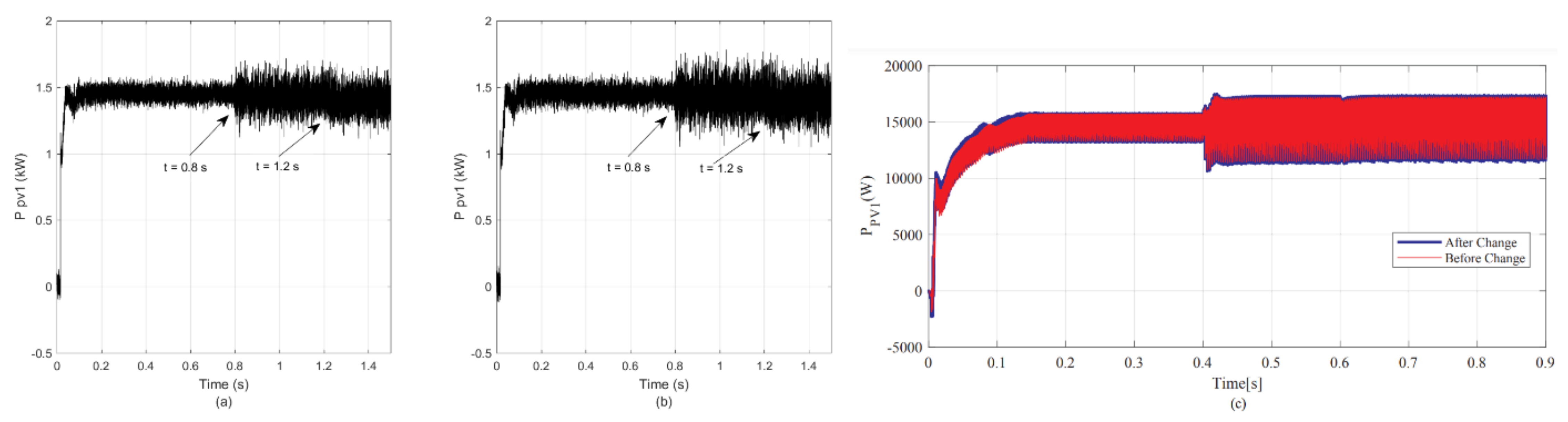
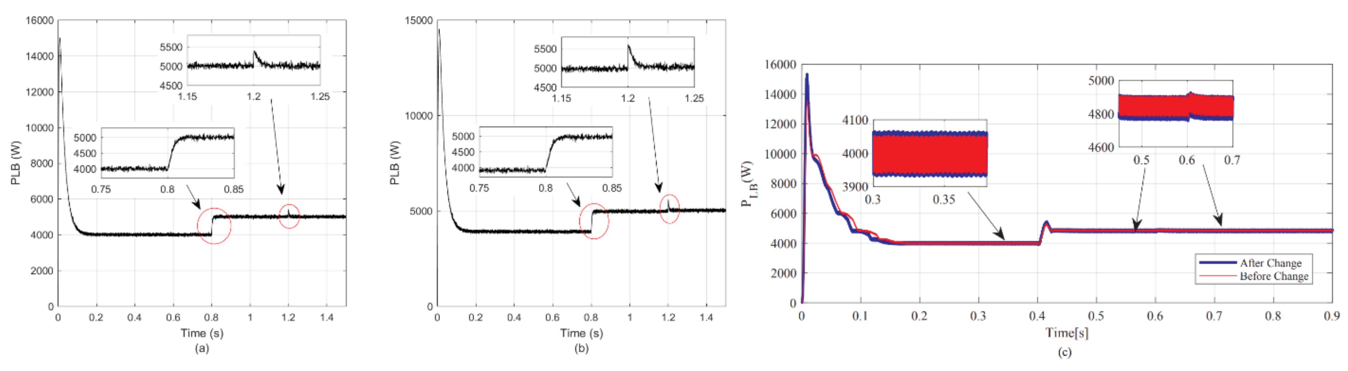
The output power of the DC/DC converter of the DC-DG2 and the bidirectional buck-boost DC/DC converter of the DC-DG2 (LB) are shown in Figure 9 and Figure 10, respectively. Both figures prove that the proposed technique effectively forces both converters to partially generate the power demanded during AC-side load changes.

In Figure 9a,b, the performance of the proposed controller with the two sets of the hybrid MG is depicted, while, in Figure 9c, the performance of the sliding-mode technique used in [19] is illustrated with small fluctuations detected in the output power of DCDG1 when the second set of parameters is applied. In Figure 10a,b, the proposed controller in the DCDG1 (LB) within the two sets of the hybrid MG is operated successfully with a dead-beat response. In Figure 10c, the sliding-mode technique used in [19] run with more significant overshoot and sluggish transient response with the second parameter’s set.

Remark 3.

The significant reduction of chattering (high-frequency signal resulting from the inverters switching) using the proposed design compared with [19] is due to utilizing the integral control in the outer loop. The swiftness and external disturbance attenuation of the proposed control is due to minimizing the ellipsoid’s volume.

4.2. Utility Grid State Variables

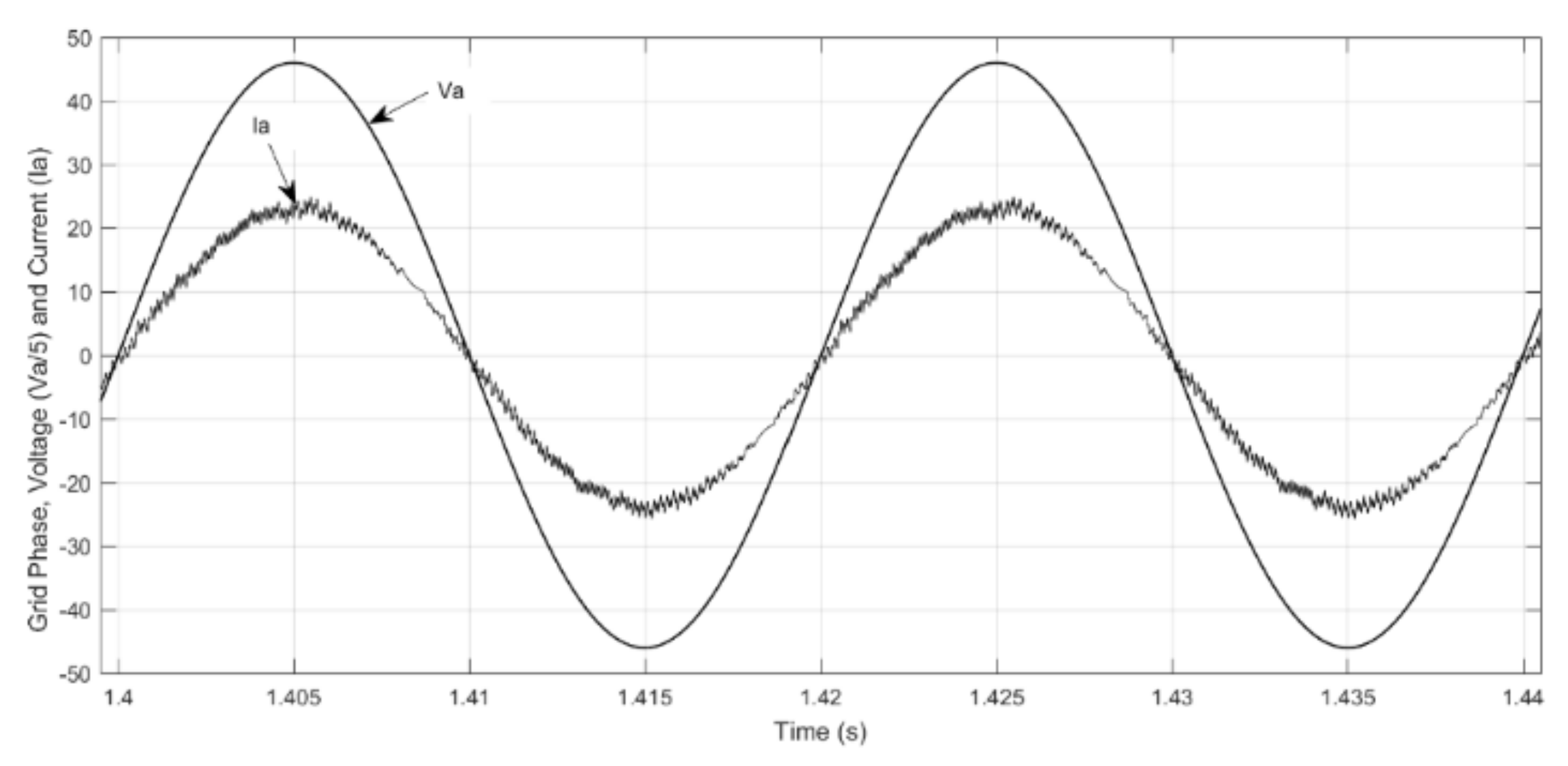
To test the proposed controller’s robustness, we have to evaluate all utility grid state variables’ responses. It is recommended to attain a unity-power factor in the utility grid. Figure 11 shows that the a-phase voltage and current are in phase. Both waveforms are sinusoidal, specifying that the power factor between the voltage and current in phase a is approximately unity. In Figure 12 and Figure 13, the utility grid frequency and magnitude of a-phase voltage under two sets of the hybrid MG system are obtained. The proposed control technique is shown in Figure 12a,b and Figure 13a,b can accurately enforce the inter-linking DC/AC power converter to preserve both grid voltage magnitude and frequency stability with an acceptable transient response. In Figure 13c and Figure 14c, the sliding-mode technique is used in [19]. The grid voltages in Figure 13c approach their desired values with more steady and dynamic errors, but they are within an acceptable range for the second set of parameters.

4.3. Power-Sharing between Converters

The inter-linking DC/AC converter must deliver a share of load power and the AC side’s uncompensated power, as demonstrated in Figure 14 and Figure 15. Based on these figures, the inter-linking DC/AC converter’s power can successfully track its desired value with less steady-state error and a swift dynamic for both sets of hybrid MGs parameters given in Table 4. Figure 14c and Figure 15c show the inter-linking DC/AC converter power-sharing of grid-connected load power for the sliding-mode technique used in [19]. The proposed technique is faster, with a dead-beat response and less chattering.

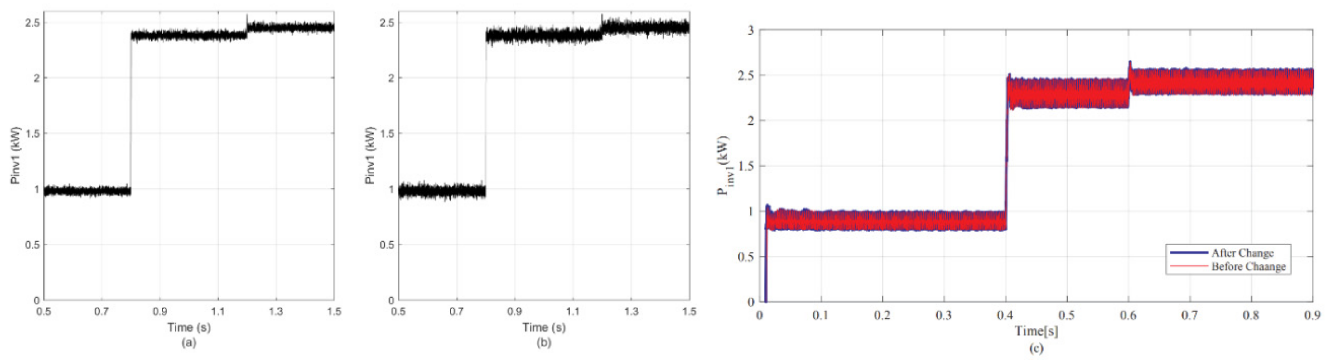
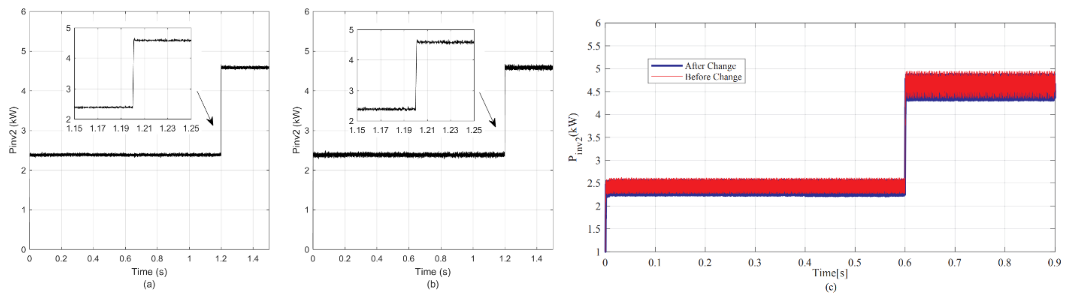
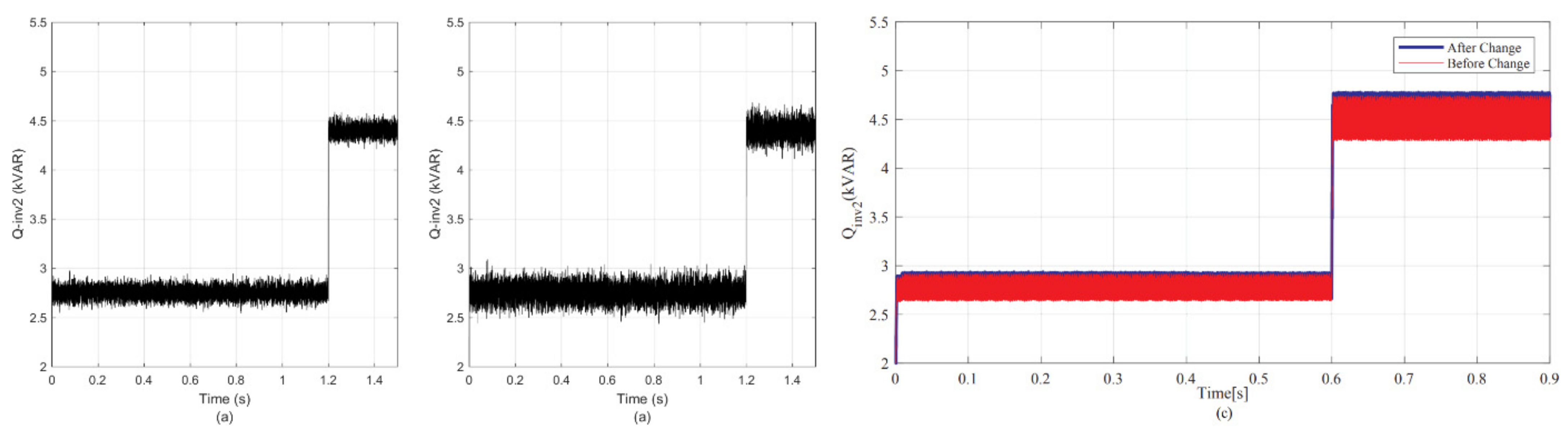
In the AC MG, the PV-inverter 1 is endorsed to provide the active and reactive power necessary for its associated local loads increased at t = 1.2 s. In Figure 16a,b and Figure 17a,b, the proposed control technique can afford stable responses for both the active and reactive power of PV-inverter 2 under both load and parameter changes. While in Figure 16c and Figure 17c, the active and reactive power of PV-inverter 2 with the sliding-mode control used in [19] are shown. The proposed technique is faster, with a dead-beat response and less chattering.

Note that the proposed controller based on the linearized model is tested on the original non-linear system in the above simulation. The proposed design is based on satisfying a set of LMIs. It guarantees the stability and disturbance rejection of the linearized model. The stability of the original non-linear system is also guaranteed according to the Lyapunov theorem. This states that the performance of both the linearized and the original non-linear system is the same (both stable or unstable) provided that the linearized model has no eigenvalues on the imaginary axis.

5. Conclusions

The paper has introduced a robust and disturbance-rejection control for hybrid MGs. The hybrid MG model is obtained and linearized. The proposed state feedback plus integral control is based on a novel sufficient condition in terms of LMIs. The design exploited the invariant ellipsoidal set. The MG model is simulated using Matlab/Simulink for different operational scenarios to verify the proposed controller’s validity. All the results are compared with a recent controller for the same model in the literature. The results confirm that the proposed algorithm, although it has a marginally slower response to the DC-link voltage, is superior in disturbance rejection, power-sharing, and power-factor correction.