Article

Physical Layer Latency Management Mechanisms: A Study for Millimeter-Wave Wi-Fi

by
Alexander Marinšek
*,
Daan Delabie
,
Lieven De Strycker
and
Liesbet Van der Perre
ESAT-WaveCore, Ghent Technology Campus, KU Leuven, 9000 Ghent, Belgium
*
Author to whom correspondence should be addressed.
Electronics 2021, 10(13), 1599; https://doi.org/10.3390/electronics10131599
Submission received: 31 May 2021 / Revised: 28 June 2021 / Accepted: 29 June 2021 / Published: 3 July 2021

Abstract

:
Emerging applications in fields such as extended reality require both a high throughput and low latency. The millimeter-wave (mmWave) spectrum is considered because of the potential in the large available bandwidth. The present work studies mmWave Wi-Fi physical layer latency management mechanisms, a key factor in providing low-latency communications for time-critical applications. We calculate physical layer latency in an ideal scenario and simulate it using a tailor-made simulation framework, based on the IEEE 802.11ad standard. Assessing data reception quality over a noisy channel yielded latency’s dependency on transmission parameters, channel noise, and digital baseband tuning. Latency in function of the modulation and coding scheme was found to span 0.28–2.71 ms in the ideal scenario, whereas simulation results also revealed its tight bond with the demapping algorithm and the number of low-density parity-check decoder iterations. The findings yielded tuning parameter combinations for reaching Pareto optimality either by constraining the bit error rate and optimizing latency or the other way around. Our assessment shows that trade-offs can and have to be made to provide sufficiently reliable low-latency communication. In good channel conditions, one may benefit from both the very high throughput and low latency; yet, in more adverse situations, lower modulation orders and additional coding overhead are a necessity.

1. Introduction

The number of connected devices is rising with a 10% compound annual growth rate (CAGR) [1], causing ever higher interference levels in the already saturated sub-6 GHz wireless spectrum. Leveraging multipath signal components and spatial diversity increases communication reliability; however, a large deal of the interference can be avoided by exploiting the 30–300 GHz millimeter-wave (mmWave) spectrum. The 270 GHz wide mmWave spectrum also allows wireless waveforms to occupy larger bandwidths. For example, the IEEE 802.11ad standard (WiGig), situated around the 60 GHz central frequency, wields 1.76 GHz wide channels [2]. In comparison, the 5 GHz IEEE 802.11ac (Wi-Fi 5) channel bandwidth is only 160 MHz [3]. Consequently, WiGig achieves data rates surpassing 8 Gbps at its highest modulation and coding scheme (MCS) setting—an enviable feat that makes mmWave Wi-Fi a perfect fit for data-hungry applications such as interactive video streaming.

1.1. The Millimeter-Wave Spectrum for Time-Critical Applications

Emerging time-critical applications in entertainment, the automotive sector, Industry 4.0 (i4.0), and healthcare require low communication latency, summarized in Table 1. Two types of latency are addressed, depending on the use case: end-to-end (E2E) latency, the communication latency between the application layers of two devices and round-trip time (RTT), the E2E delay with the addition of a response.
Comprised of interactive and immersive applications, extended reality (XR) requires a large throughput. Rendering scenery in life-like detail, and depending on external factors such as video resolution and compression, the requirements range from tens of Mbps [5] to several Gbps [11,12]. While XR devices can compensate low data rates with elastic services [13], having a human in the loop means they have to always comply with a certain latency constraint. The latter ranges roughly from 100 to 1 ms, depending on the user mobility [14,15], XR device [16], and physiological parameters [17]. However, most of the XR applications have either got a 20- or 10 ms latency constraint. Two examples are virtual reality (VR) entertainment and telesurgery using augmented reality (AR) or mixed reality (MR).
Following the growing amount of real-time data sharing fuelled by the pursuit for the widespread edge- and fog computing adoption, mmWave frequencies are increasingly being considered by other emerging applications. Among them are vehicle-to-everything (V2X), unmanned vehicle (UV) and drone communications. Their further dissection yields specific allowed latency regions, for instance, in platooning, remote control, cooperative driving, and collective information sharing scenarios as shown in Table 1.
The same applies to i4.0 where, for example, numerous collaborating robots on a factory floor can leverage highly directive mmWave data links to avoid interference. Digital twins and real-time control, on the other hand, are examples of applications requiring a high throughput. Whether XR, V2X, or i4.0, all the above-mentioned applications can benefit from mmWave communication systems, given they provide low-latency operation.

1.2. Related Work on Latency Reduction

WiGig’s contribution to latency has already been debated in several other works in the past. For example, in mapping the E2E latency between the application layers of two devices, the authors of [18] established that 10–15 ms time delays are typically encountered in indoor scenarios with a direct line-of-sight between the two communicating devices. The results obtained using the ns-3 network simulator are roughly similar to the experimental findings in [19,20,21,22]. All of these studies elaborate on the appropriateness of WiGig for serving XR applications, receiving high-resolution video streams over the network. Their approach to latency reduction includes combining WiGig with sub-6 GHz Wi-Fi [22], dynamically tuning the video encoder [20], synchronising data transmission with application-specific events [21], and leveraging user pose information for quicker beam- and access point (AP) switching [19]. As a result of these latency mitigation strategies, the range of expected latency values of individual video frames gets extended to 5–50 ms. Regardless of how successful such top-down approaches are in latency reduction, they are all limited by the underlying network layers. As demonstrated in [23], even sub-10 ms session transfer time delays in the MAC layer generate up to two orders of magnitude higher delays in the transport layer. Hence, optimizing the lower network layers is crucial both for reducing overall latency and understanding the recorded time delays, when looking from the top down.
The above-mentioned AP hand-offs and session transfers between WiGig and Wi-Fi are one of the more commonly-optimized IEEE 802.11 MAC layer mechanisms, influencing transmission time delays. Others include augmenting the automatic repeat request (ARQ) scheme [24], leveraging aggregation of frames and of the already aggregated data to decrease the overhead [25], and using multiple distributed APs for even higher data rates [5]. However, except for associating the finite physical layer (PHY) data rates with transmission delays [26], there is a general lack of IEEE 802.11 PHY latency models and understanding of the underlying latency management mechanisms.
Broader studies discussing the implications of the PHY on transmission latency [27] note the importance of adaptively setting the MCS based on the latest channel state information (CSI). Doing so increases the average throughput and, therefore, reduces transmission times. The authors also elaborate on the importance of short packets in view of timely data delivery, although, the approach may not be entirely applicable to the likes of XR video streaming applications because of their high throughput demands. Among other radio access technology (RAT) options, 5G new radio (5G NR) has been putting increased emphasis on the PHY and its role in ultra-reliable and low-latency communications (URLLC). It aims for a 1 ms small packet latency while keeping bit error ratio (BER) values below 10 5 [28]. The main challenges 5G NR URLLC faces are reducing the transmission time of a single packet and achieving better control over individual packet processing times [29]. Although 5G NR URLLC tackles latency reduction by introducing new packet formats, it has several things in common with IEEE 802.11ad. For example, both standards employ iterative low-density parity-check (LDPC) decoding, which makes up a substantial part of the packet processing time and is identified as both a key enabler of 5G NR URLLC systems [30] and one of the potential optimization points [29].

1.3. Physical Layer Latency Probing

Providing sufficient latency containment mechanisms for tomorrow’s real-time applications is not a trivial task. Every layer in the communication stack has its own level of flexibility. Sometimes, the latency accumulated in a single layer is also dependent on other layers. Starting from the bottom up, the present work studies latency accumulation from the perspective of the PHY. It considers both transmitter (TX) and receiver (RX)-based latency management mechanisms to determine the resulting range of expected latency values. The PHY component performance figures are derived from research efforts concerning integrated circuit (IC) design and are implemented in a tailor-made 802.11ad PHY simulation framework. Alongside the time delay results, the effects of latency mitigation on data integrity are evaluated. The three-fold contribution of the present work is summarized below.
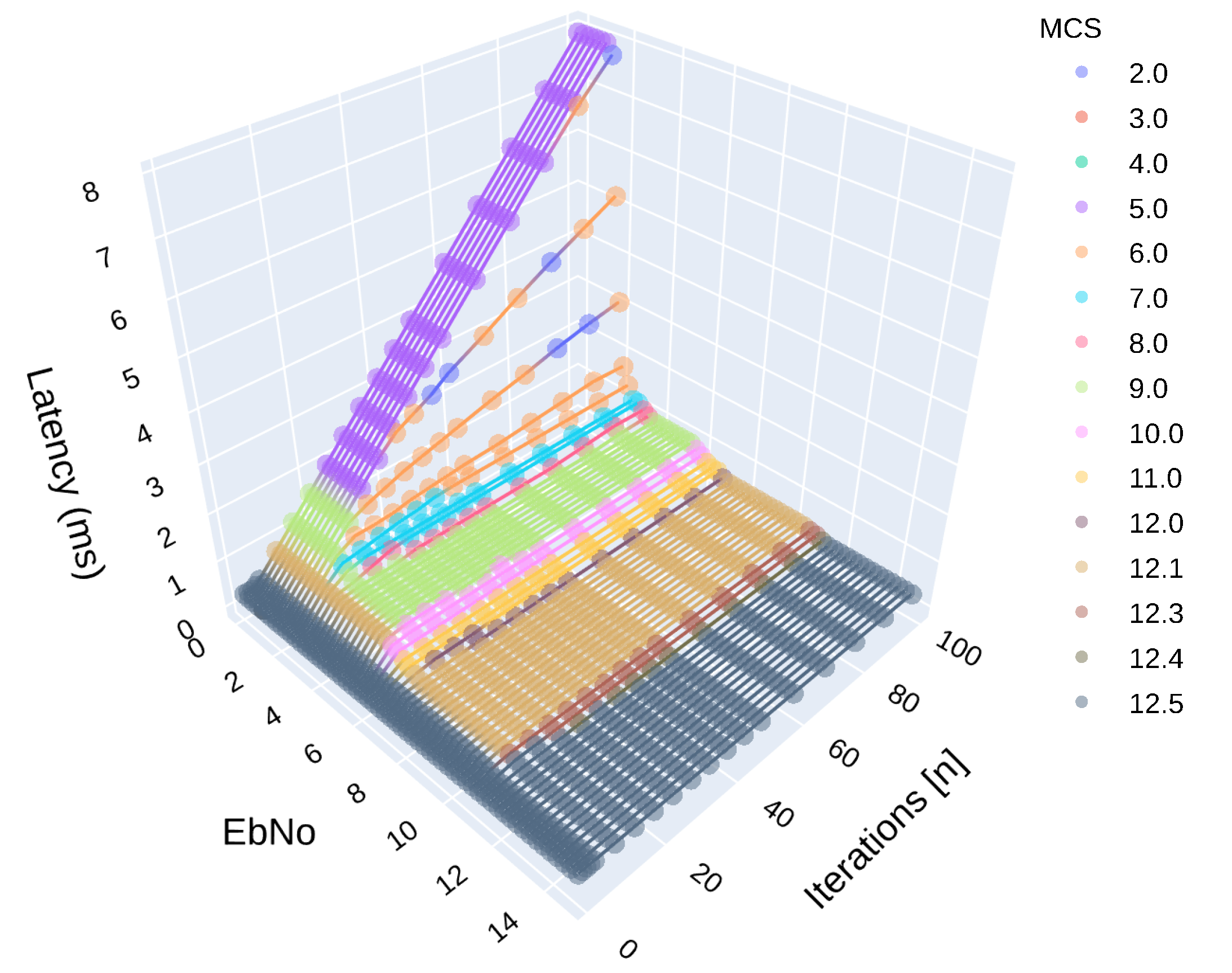
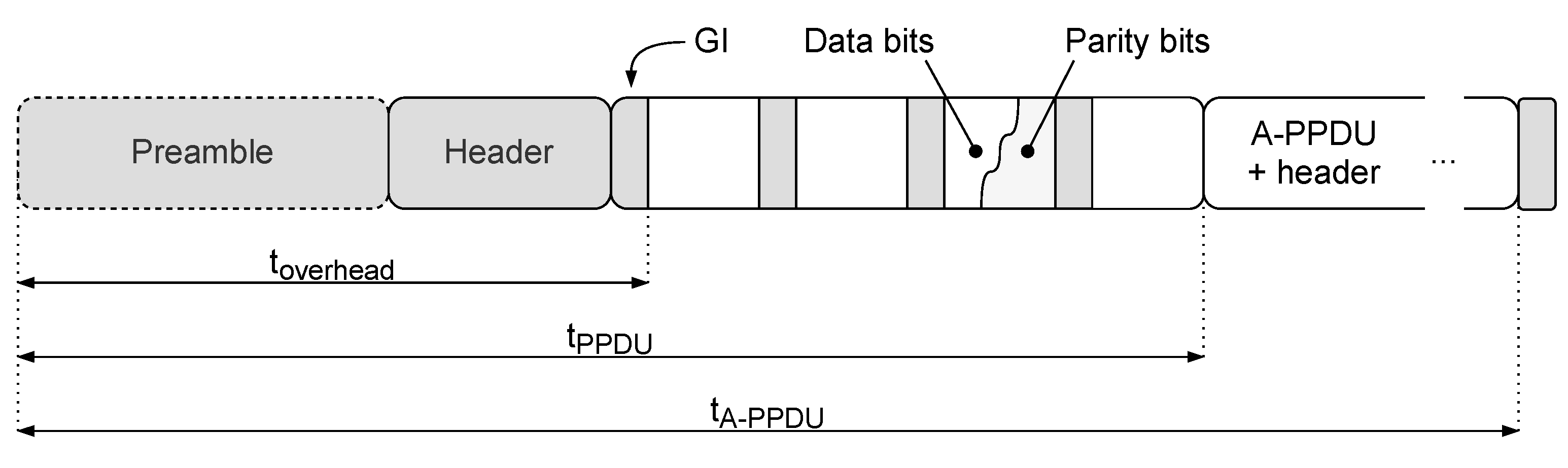
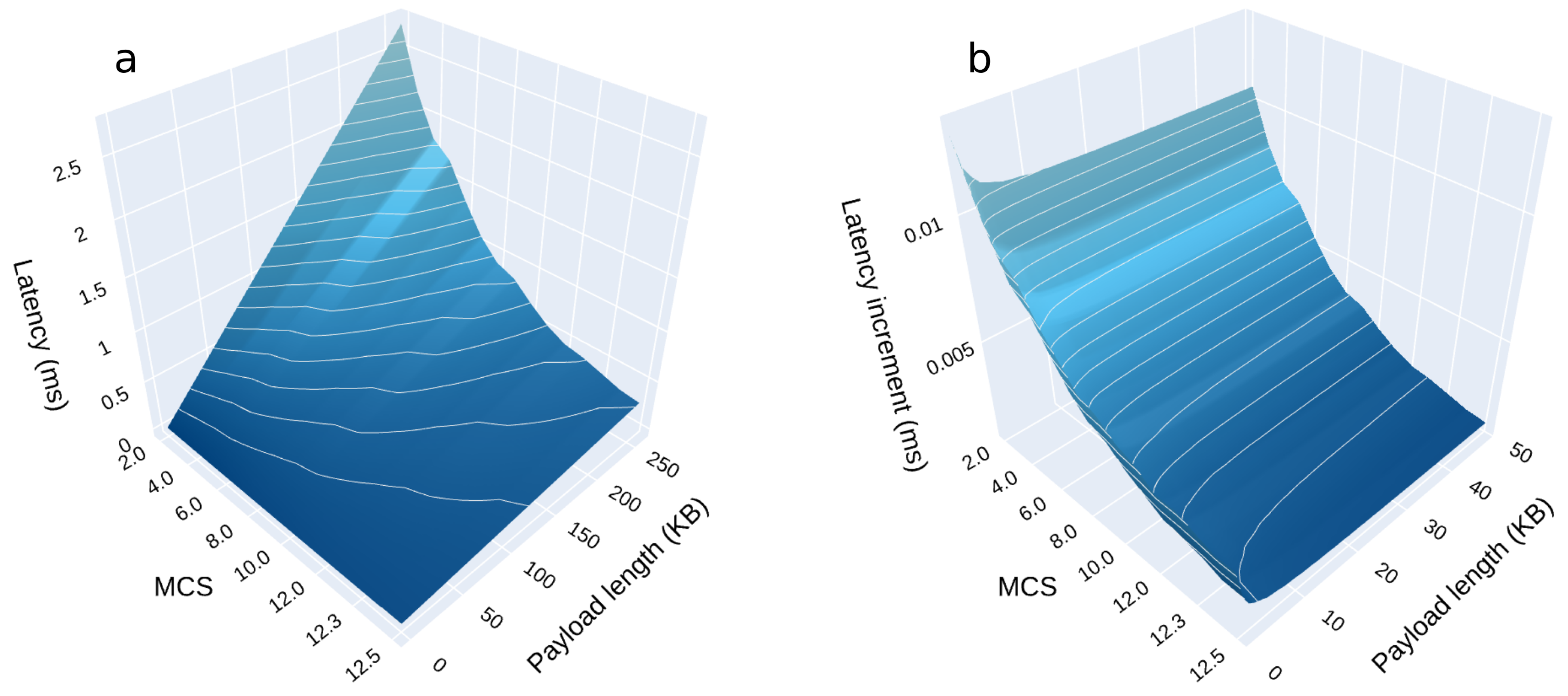
  • PHY latency analysis: The dependency of time delays on PHY protocol data unit (PPDU) payload length, PPDU aggregation, the selected MCS, the employed demapping algorithm, and the number of LDPC decoding iterations is established
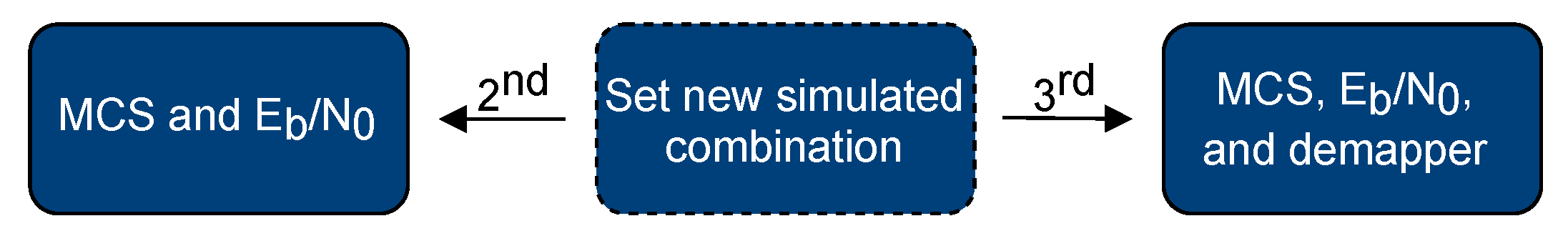
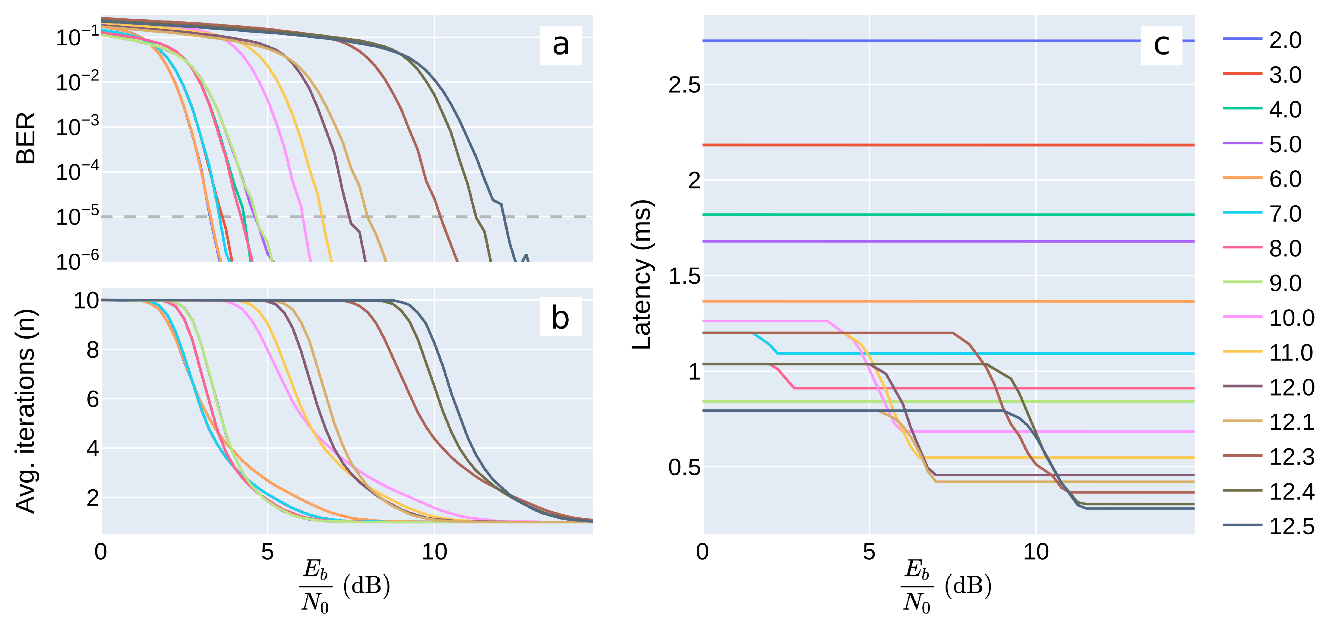
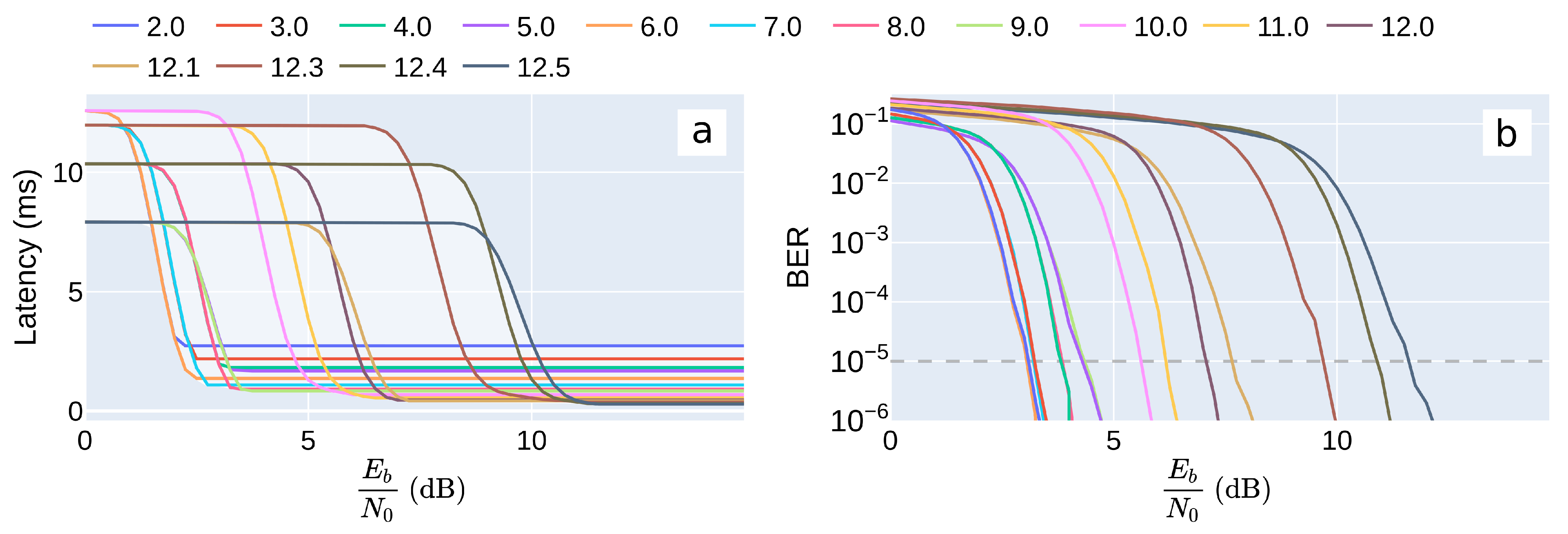
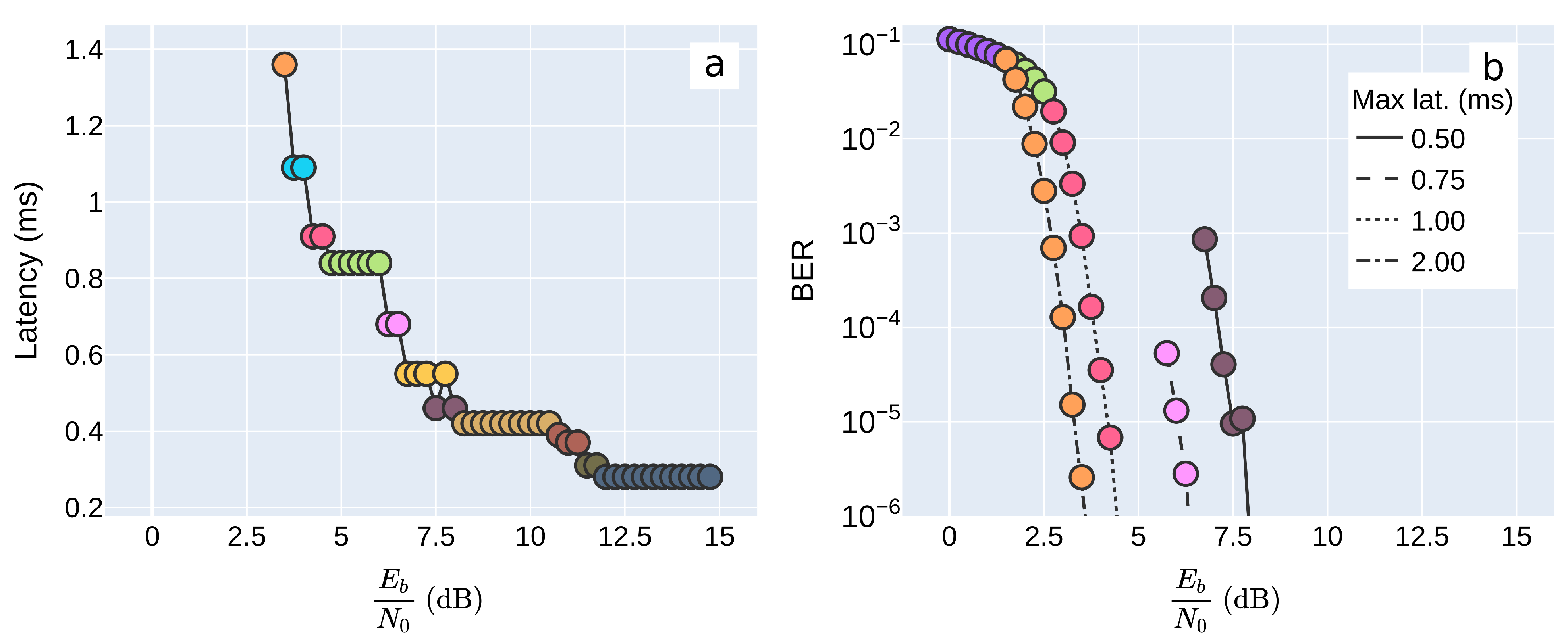
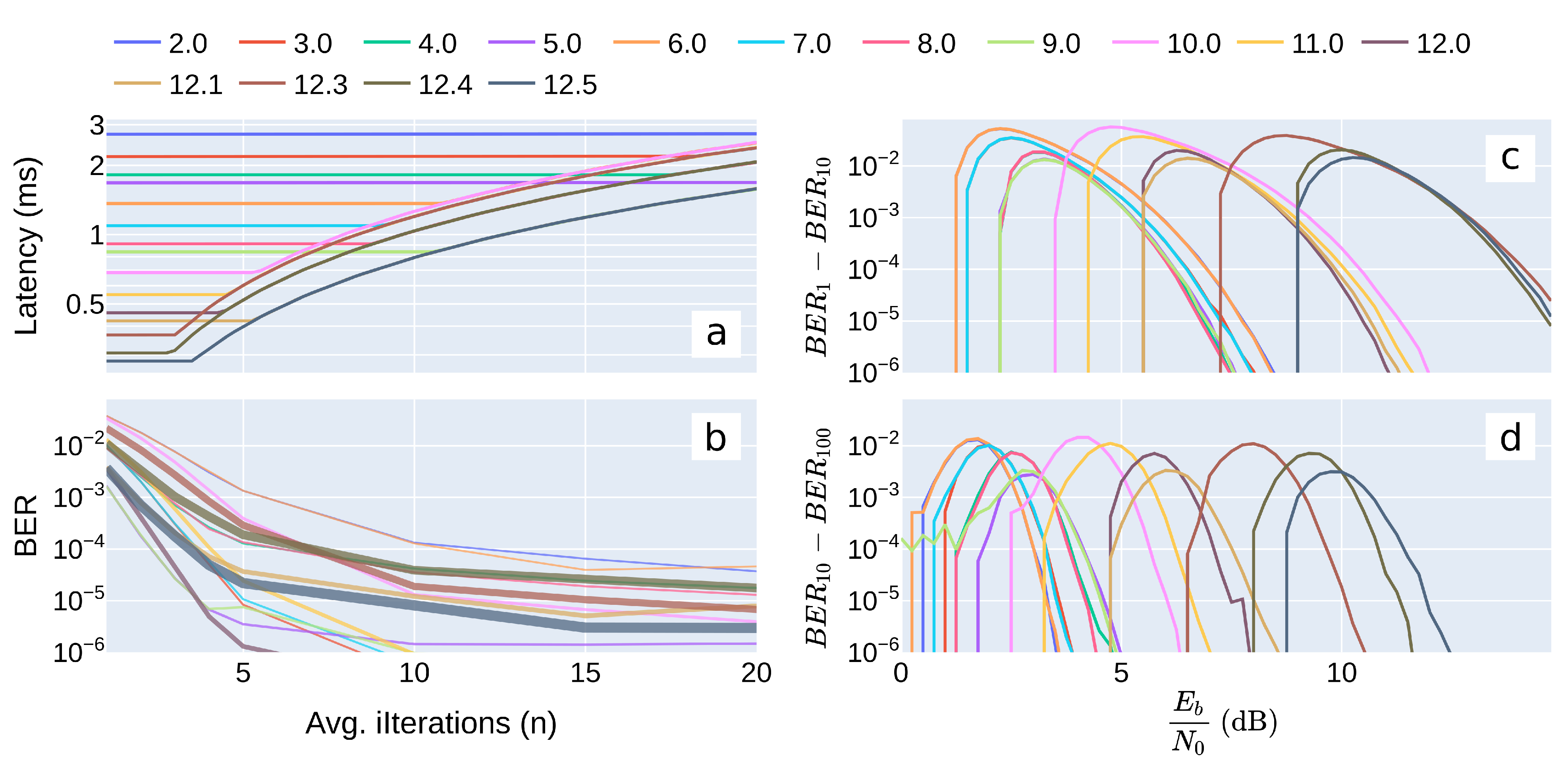
  • Latency management mechanisms: Data transmission over an additive white Gaussian noise (AWGN) channel is carried out to study the trade-offs between the incurred latency and the resulting BER. The lowest achievable latency is determined in relation to PHY tuning parameters and using 10 5 as the BER constraint. Moreover, Pareto optimality in achieving minimal BER is addressed in light of different latency thresholds.
  • Simulation framework: An open-source IEEE 802.11ad PHY latency and BER simulation framework has been designed during the course of the study. It closely complies with the WiGig standard, offers flexibility for future studies, and is shared in open access.
The target latency performance metric and the derivation of the ideal case time delay, assuming infinite processing speed, is presented in Section 2. Associating the PHY’s components with realistic performance figures sourced from state-of-the-art literature is described in Section 3, while Section 4 touches upon the inner workings of the simulation environment and outlines the workflow adopted for the purpose of generating the latency and BER results. The simulation results are contained within Section 5, whereas their inter-dependencies are discussed in Section 6. Finally, Section 7 summarizes the findings and highlights potential future research prospects.

2. Latency Definition and the Ideal Case Study

Ideal case latency is studied initially, evaluating the effects of TX tuning—MCS selection, payload length, and PPDU aggregation—on time delays. However, the latency performance metric is defined first.

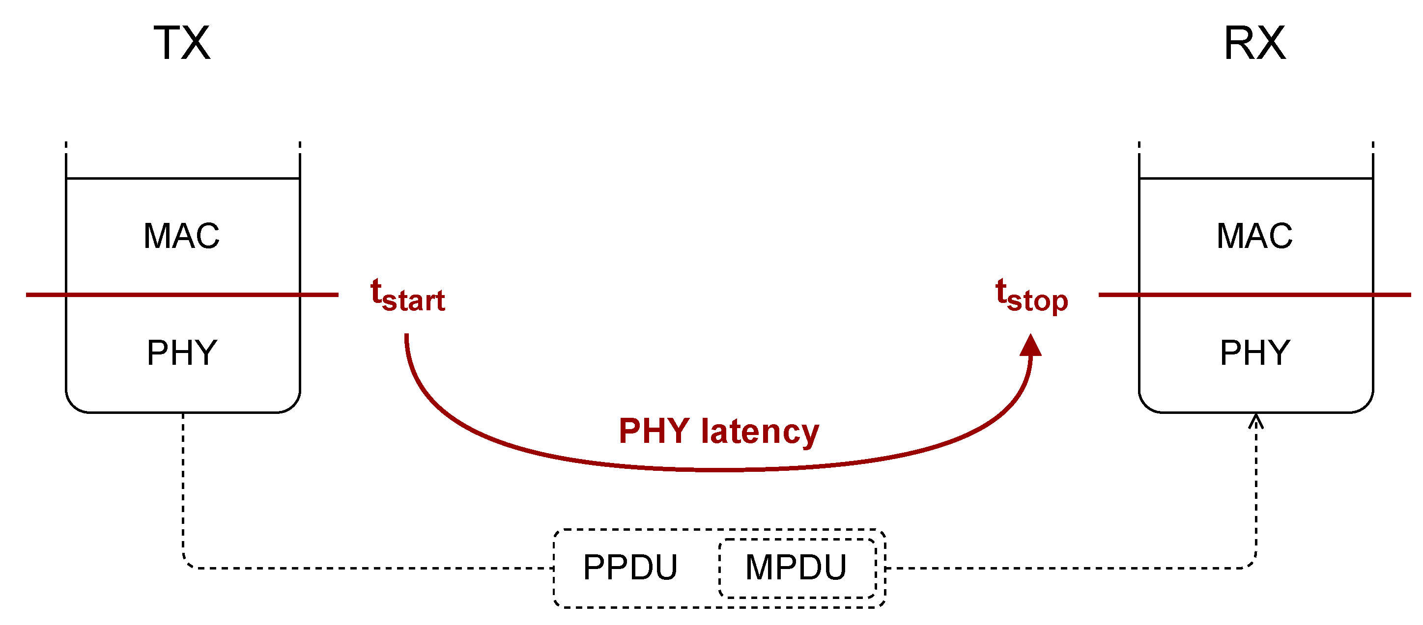
2.1. Physical Layer Latency

The present work defines PPDU payload latency as the target performance metric, focusing solely on latency incurred in the PHY. This encompasses the processing time at the TX and RX digital basebands (DBBs) and includes data propagation through the channel. It is analogous to tracking the E2E delay of individual MAC layer protocol data units (MPDUs) (the terms PPDU payload and MPDU are used interchangeably in the manuscript). from entering the TX PHY, to exiting the RX PHY and heading upwards through the network stack. Marking the timing start and stop points, Figure 1 depicts MPDU propagation and the latency it encounters through the PHY.

2.2. Analytical Derivation of Latency in the Ideal Scenario

The only contribution to latency in an ideal scenario is caused by the finite signal bandwidth and the propagation speed of electromagnetic waves. All data processing in the PHY is assumed to be instantaneous. The data propagation speed through the channel comes close to 3 × 10 8 ms 1 when traveling through air. The resulting time delays are less than 100 ns at practical mmWave indoor communication distances of up to 30 m. Consequently, electromagnetic wave propagation delays are discarded early on.
The remaining delay is attributed to the finite symbol rate of the communication standard. With the IEEE 802.11ad channels occupying 2.16 GHz of the spectrum and providing 1.76 GHz of usable bandwidth, the symbol rate is limited to 1.76 Gsps. As a result, individual symbols take up roughly 0.57 ns of airtime. The otherwise small delay is magnified by long symbol sequences, prepended to the packet payload. The 4416-symbol long preamble, header, and initial guard interval (GI) cause a 2.5 µs delay to the first data payload symbol. This delay further increases for each succeeding symbol by the sum of individual symbol delays before it, which also include a GI, prepended to every block of 448 data symbols. The worst case symbol delay dictates the total packet delay. Depicted in Figure 2, the waiting time for a single PPDU is associated with the reception of all of its data bits and the corresponding overhead. The preamble is skipped in aggregated PHY protocol data units (A-PPDUs).
Reducing the MPDU delay is directly achieved by shortening the MPDU itself. Secondly, switching the modulation and coding scheme (MCS) will provoke different amounts of coding overhead and determine the number of bits carried per symbol. The ideal scenario analysis initially studies the combined MPDU length and MCS effects on MPDU latency. Equations (1) and (2) describe the incurred latency:
L a t e n c y P P D U = ( L P + L H + L D + 64 ) 1.76 Gsps
L D = l 672 · R c 672 448 · R m · 512
where L P , L H , and L D represent the length of the preamble, header, and data in symbols. Together with the final GI, and divided by the symbol rate, they yield the packet’s latency. The length of L D is calculated on the basis of the payload data length (l), code rate ( R c ), and modulation rate ( R m ). L P and L H take up 3328 and 1024 symbols, accordingly. The evaluated MCSs are listed in Table 2.
Following the first part of the ideal case study, the payload length has been set to the highest value supported by the IEEE 802.11ad PHY, 262.143 kB. This applies to all subsequent study steps. Long PPDU payloads are studied with the goal of analyzing high-throughput low-overhead transmission in more detail. Moreover, emphasis is put on XR use cases, where the data-hungry interactive streaming applications require multi-Gbps data rates. This is also the worst-case latency, as longer packets inherently feature longer transmission delays. Therefore, time-critical applications that require shorter payload transmission are expected to achieve lower latency. Given a 10 5 BER, every 262 kB packet on average includes 21 bit errors. Real-time streaming applications in general allow for a certain extent of erroneous data as long as their throughput and latency requirements are met. Consequently, the 10 5 BER threshold is kept as a reference throughout the manuscript.
In PPDU aggregation, multiple PPDUs and their headers are appended to a single preamble. This decreases the relative overhead, while latency is described by Equation (3):
L a t e n c y A P P D U = ( L P + N · ( L H + L D ) ) 1.76 Gsps ,
where N stands for the total number of aggregated packets preceding the observed A-PPDUs.

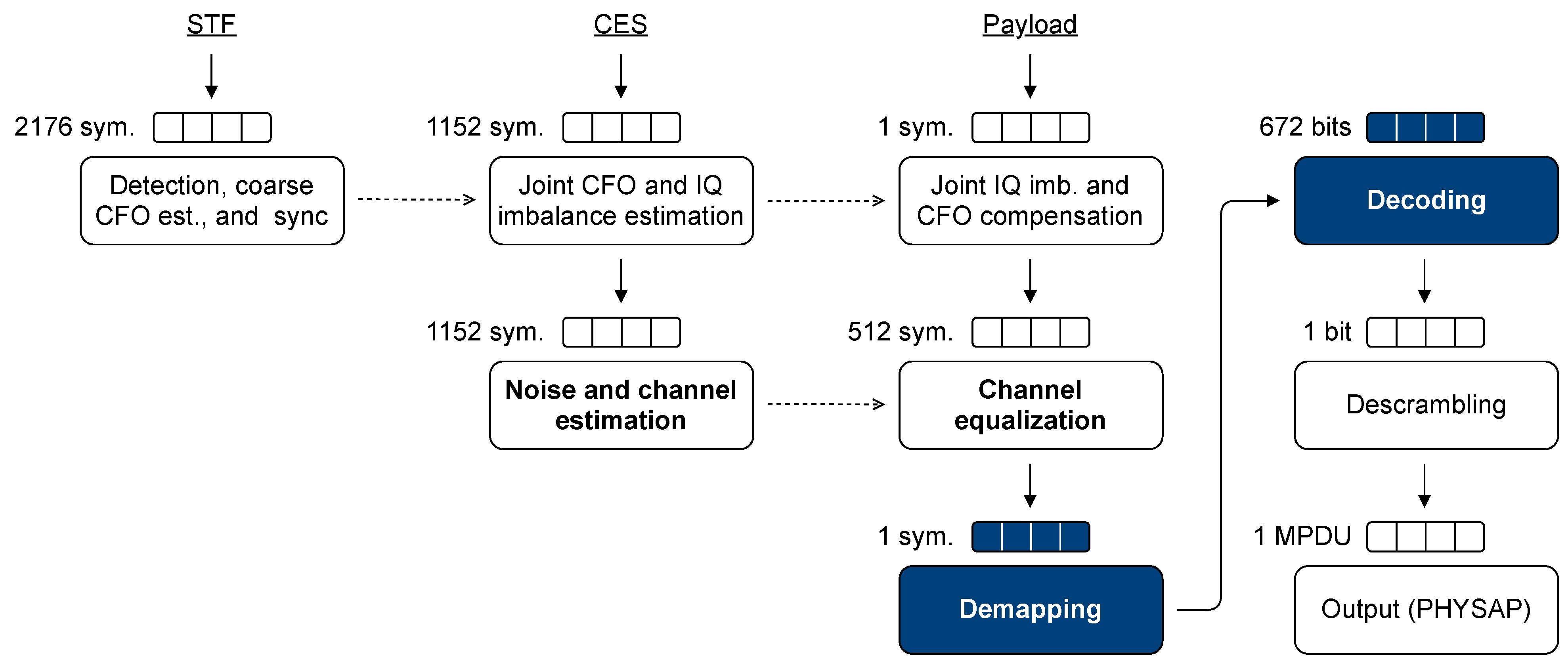
3. Latency-Inducing Receiver Digital Baseband

The TX and RX both need to comply with the IEEE 802.11ad PHY standard, which is especially important for the TX as it should correctly prepare packets for transmission, use the appropriate waveform, and stay within transmission power limitations. Its main contribution to latency is the 1.76 Gsps finite transmission data rate. This study assumes that data are prepared for transmission using high-throughput components [31], avoiding any potential bottlenecks. Moreover, any processing delay is compensated for by formatting the data during preamble and header transmission, filling the transmission buffer with payload symbols in real-time.
The RX, on the other hand, is only responsible for correct data reception; the path it takes to achieve this goal is left to the system designers to determine. Several common RX DBB design solutions exist, depending on how the RX DBB blocks are organized, which signal domains are used, and how timely or accurate data reception is. The RX DBB used in this work operates in single carrier (SC) mode and employs frequency domain equalization (FDE). It is roughly based on the work presented in [32], while Figure 3 outlines its design.

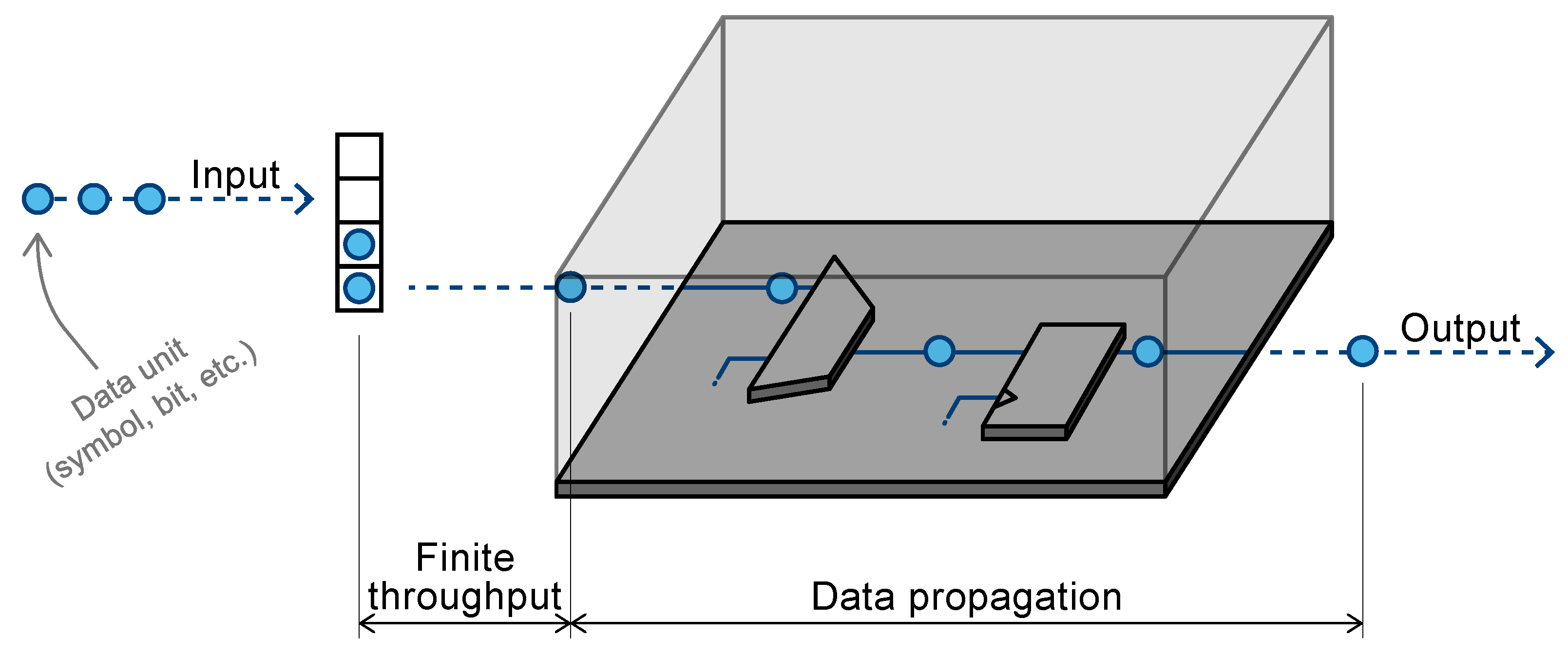
3.1. Two Distinct Time Delays

Latency incurred in the RX DBB originates from data propagation time delays and finite throughput values of individual components. The former represents the time a data unit, e.g., a bit, has to spend in the component before exiting it, while the latter stands for the elapsed time between two consecutive data units entering the component. The finite throughput delay is only applied to data arriving at a busy component, where the waiting time is a multiple of the throughput delay and the number of queued data elements. Only data propagation delays apply for data passing through otherwise idle components. For example, the first data element in a stream. Figure 4 illustrates both delays on a simplified example. The input data units can be symbols, bits, or data blocks, depending on the assessed component. A component’s throughput must reflect the rate of incoming data to avoid becoming a bottleneck, while data propagation delays will add latency to the entire stream of data. The work at hand models individual components as black boxes, with the finite throughput and data propagation delay influencing the flow of data through it. The interplay of multiple components and their time delay performance figures yields the total latency incurred in the RX DBB.

3.2. Performance Figure Derivation

The RX DBB components are in the present study based on best-in-class 65 nm IC designs found in literature, except for the exact- (28 nm) and approximative demapper (90 nm)—elaborated on in the corresponding subsection. The reported data propagation delays and finite throughput values are associated with the components making up the assessed RX DBB. However, other IC component implementations exist and might yield different latency results. The present work acknowledges IC design is a fast-evolving field and instead focuses on studying latency mitigation mechanisms, which are universally applicable.
Given the separation of input data in Figure 3 into three types—short training field (STF), channel estimation sequence (CES), and payload—and the performance of the corresponding ingress components, the following sections assume their negligible contribution to latency. The remaining components contribute to MPDU latency through the data propagation time delay and finite throughput performance metrics. Except for the (de)scrambler, which does not significantly contribute to latency owing to the simplicity of the (de)scrambling function and state-of-the-art component throughput values surpassing 25 Gbps [33].

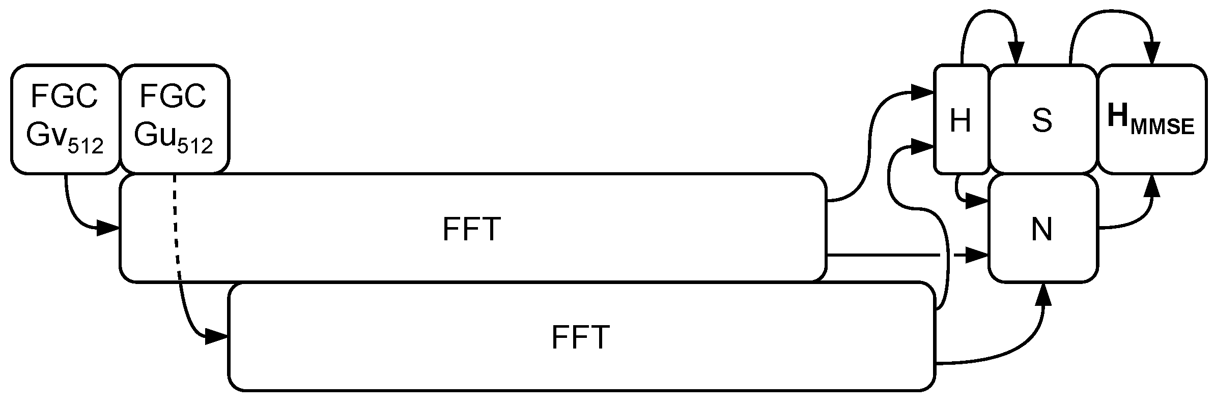
3.2.1. Noise and Channel Estimator

The channel and noise estimation block’s primary purpose is to estimate the minimum mean square error (MMSE) channel equalization tap weights, achieved by uniting several operations. Its noise estimates are also an important factor in soft-decision demapping. The noise and channel estimation tasks include:
  • Using the fast Golay correlation (FGC) algorithm [34] to calculate the cross-correlation between the received signal and the two known complementary Golay sequences G v 512 and G u 512 . The process is repeated twice—once for each Golay sequence—and ultimately yields the channel input response (CIR).
  • Converting the FGC results to the frequency domain via a fast Fourier transform (FFT) block, weighing them with 1 2 , and adding them together, forming the channel frequency response (CFR).
  • Calculating the signal-to-noise ratio (SNR) using the CFR and the frequency-domain correlation results.
  • Finally, obtaining the MMSE matrix using the CFR and SNR.
The above tasks are illustrated in Figure 5, which roughly outlines their time delays and parallel execution possibilities. Based on these, the study assumes the FFT is the most time-consuming factor in the noise and channel estimation block. The FFT’s throughput and propagation delay are derived from [35], where the authors report a 2.64 Gsps output sample rate and a latency from the input to the output of 63 cycles. Using the same clock frequency as in their work—330 MHz—results in a 191 ns propagation time delay.

3.2.2. Channel Equalizer

The discussed RX DBB employs single carrier frequency domain equalization (SC-FDE). However, before neutralizing the channel effects, the received symbols must be transformed to the frequency domain. Once a block of 448 data symbols and its 64-symbol long cyclic prefix (CP) have accumulated at the input of the channel equalization block, they are transferred to the frequency domain using the same 512-point FFT [35] component, as described in Section 3.2.1. Multiplying the inverse of the CFR with a block of received symbols in the frequency domain, the equalization itself takes the form of parallel complex multiplications. Executing the multiplication and corresponding summations alleviates most of the time delays, making the FFT the main factor contributing to latency. Lastly, the 512 equalized symbols are transferred back to the time domain by an inverse fast Fourier transform (IFFT). Given the same processors are often used for both time-to-frequency and frequency-to-time domain transformation, the same performance metrics are associated with both the FFT and the IFFT component. Thus, the total propagation delay of the channel equalization block is that of two FFT/IFFT components. Its throughput is limited by that of a single FFT/IFFT component.

3.2.3. Symbol Demapper

The described RX DBB employs one of three demapping algorithms. All of them convert a single received symbol into a sequence of log-likelihood ratio (LLR) values. These represent the probability that the corresponding bit in the symbol constellation is a one or a zero. The length of the output LLR sequences is equal to the modulation rate.
The three algorithms and their performances for 16QAM are listed in Table 3, where δ 2 is the noise variance, M the constellation size, and r the received symbol. The i-th constellation point where the k-th LLR is either 0 or 1 is represented by C i , 0 or C i , 1 , respectively.
The first equation represents the exact LLR calculation algorithm. Since the authors used a field-programmable gate array (FPGA) for the purpose of their study, the throughput has been increased by a factor of 3.2—the average increase in application throughput when migrating from an FPGA to an application-specific integrated circuit (ASIC) implementation [39]. This is the only time when the normalization factor was applied, as all other component performance figures correspond to ASIC-based designs. The difference in process nodes between the demappers was not compensated due to the lack of an explicit scaling factor. Note should be taken that the approximative demapper is implemented in 90 nm technology, and its implementation using a 65 nm process could increase transistor density [40] and decrease propagation delays [41]. Consequently, the approximative demapper latency results should be assessed with some reserve since a 65 nm implementation could increase the component’s throughput. The opposite is true for the exact demapper, deriving its throughput from a 28 nm implementation. Next from top to bottom is the approximative algorithm. Although simplified, the algorithm still needs to iterate over all the constellation points for every received symbol. Lastly, the decision threshold algorithm simplifies the demapping procedure by grouping constellation points into clusters and working only on the basis of those. This makes it the fastest of the three.
In the studied demapper implementations, only the throughput delay is considered since it is the main performance metric noted in [36,37,38]. The delay manifests itself as the time between the processing of consecutive input symbols. Consequently, a symbol rate higher than the demapper’s throughput will cause symbols to start piling up at the demapper’s input. This would prevent the RX DBB from processing input symbols at the standardized 1.76 Gsps rate. Therefore, the simulated RX DBB uses 5 demappers in parallel. After removing the GIs, the parallel decision threshold demapper manages to surpass the data symbol rate by a small margin. The remaining two parallel demappers—exact and approximative—rely on more complex processing, reflected in their lower throughput.

3.2.4. LDPC Decoder

The decoder leverages redundant parity bits within each codeword for iterative forward error correction (FEC), operating on the received LLR values. Increasing the number of iterations decreases the probability of bit error propagation further through the RX DBB [42,43]. However, fewer iterations yield shorter time delays.
The IEEE 802.11ad LDPC codewords consist of 672 bits, whereas the resulting dataword length at the decoder’s output depends on the code rate. To accurately model the corresponding delays, the performance figures are derived from [44], where the authors report a 5.3 Gbps throughput and a latency of 150 ns for 5-iteration 13/16-code-rate decoding. They also make note of the number of processing cycles consumed per iteration for all code rates, except 7/8. The latter is thus not part of the present study. The described performance figures lead to the delay functions contained in Equations (4) and (5):
T D ( R c , i ) = 5.3 Gbps · 10 9 · 13 C ( R c ) 1 · i 5
P D ( R c , i ) = 150 ns · 1 4 + 3 4 · C ( R c ) 13 · i 5
where T D and P D represent the throughput- and data propagation delay, R c is the selected code rate, C ( R c ) stands for the number of incurred processing cycles, and i marks the number of incurred decoding iterations. T D and P D both depend on the ratio between C ( R c ) and the number of iterations for the reference code rate, 13 when R c = 13 16 . Moreover, they are governed by the quotient between i and 5, the reference number of iterations studied in [44]. A constant 25% of the reported propagation delay is assumed to be latency caused by buffering, memory access, and I/O operations. The remaining propagation delay factor scales with the code rate and number of iterations.

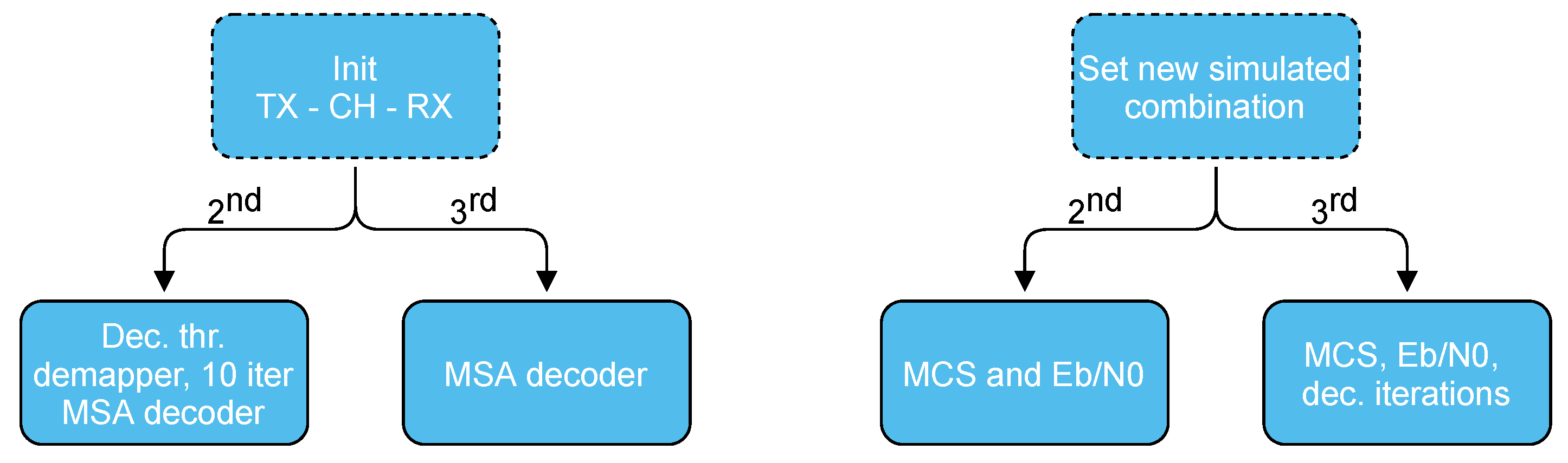
4. Simulation Environment

A simulation framework has been designed as part of the present work. It consists of both latency probing, described in [45], and data transmission over a noisy channel. Together, they allow joint latency and BER analysis.
The RX DBB, discussed in Section 3.2, is implemented alongside the TX DBB, forming the IEEE 802.11ad transmission chain together with an AWGN channel (CH). The TX includes scrambling, encoding and mapping of the data bits, while providing all additional PPDU overhead structures in preparing PHY frames for transmission. The AWGN CH adds noise, and the inverse of PPDU generation is carried out at the RX. The latter also implements the time delay functionalities of individual components, described in Section 3.2.1, Section 3.2.2, Section 3.2.3 and Section 3.2.4. The simulation framework is written in Python, and apart from SimPy, relies on conventional scientific computing libraries such as Numpy, Pandas, and Xarray. It implements unit tests to verify the correctness of individual component definitions. Where possible, the results of these are evaluated against those obtained using MATLAB’s Communication Toolbox.
Transmitting millions of data bits upon every possible change in the TX-CH-RX chain can be a daunting task. The use of the SimPy discrete-event simulation framework may provide accurate latency tracking, yet, it further increases the already long computation time. We have split the simulation into error tracking and separate latency probing to accelerate execution. Moreover, it provides easier reproducibility of results by allowing better control over the simulated scenario and its input arguments. Summarized in Figure 6, the first part tracks the quality of the received data in different channel conditions while also storing the number of incurred decoding iterations. These are then used to initialize the latency simulation. The decoupled approach alleviates the need to run numerous event-based packet transmission simulations for each input parameter combination.
Figure 6 shows the simulation workflow for assessing PHY latency. It is initially used to assess latency and the incurred BER in presence of an AWGN CH, using the decision threshold demapper and limiting the number of decoding iterations to 10. It is afterwards used in an exploratory study, focusing on RX tuning by switching the demapping algorithm and allowing up to 100 iterations. In sequence, the ideal scenario study is referred to as study step 1, while the two simulation steps are referred to as steps 2 and 3. The naming is used in the following subsections to describe how the simulations are configured during the different study steps. The simulation framework is publicly accessible (individual repositories are located at https://github.com/PhyPy-802dot11ad, accessed on 31 May 2021) and consists of: IEEE 802.11ad component functionalities, the latency simulator, and the BER simulator.

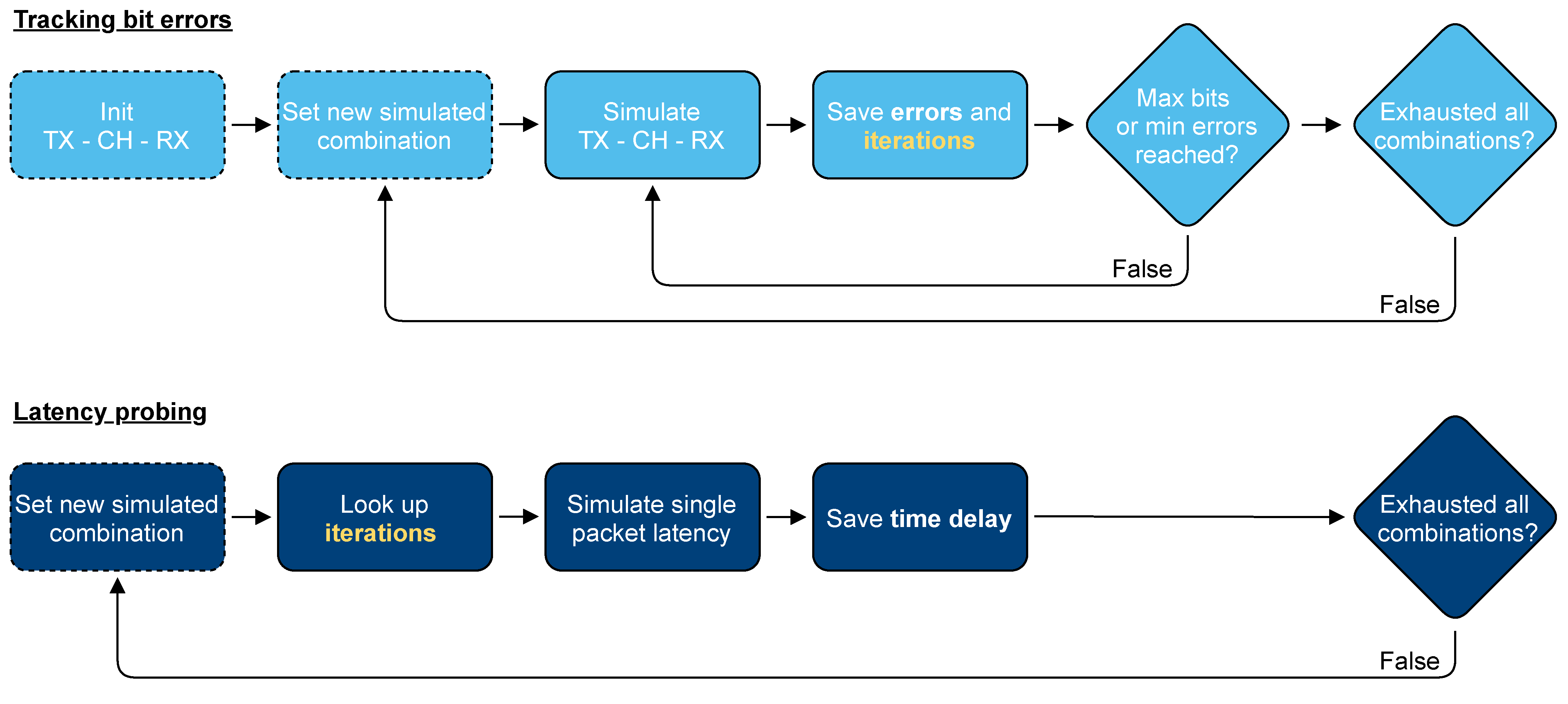
4.1. Tracking Bit Errors

The first part of the simulation process is conceived of encapsulating an MPDU in a PPDU, before exposing it to AWGN. The distorted sequence is then demapped, decoded, descrambled, and compared to the initial sequence. The process is repeated till an adequate number of bit errors is reached or the maximal allowed number of bits has been transmitted. The two values are set to 100 and 10 8 , respectively. The only exception is that at least 3 PPDUs must be successfully received before the simulation is allowed to terminate. This results in the generation of up to 48 random MPDU sequences spanning the longest supported PPDU data payload length (262 kB). The Monte Carlo simulation is repeated for each input MCS and E b N 0 combination. Upon every PPDU transmission, the number of bit errors, the individual packet error, and the average number of decoder iterations over all codewords is stored.
Pointed out by Figure 7, two blocks in the simulation framework change between the two study steps. In step number 2, the decoder may execute up to 10 decoding iterations, and exit prematurely if the early exit criterion is met. The criterion allows the decoder to stop execution if no bit errors are detected in the received codeword [46]. It is not altered during the simulation, as only the MCS and E b N 0 combinations are changed. Step 3 adds decoder tuning, sweeping the number of allowed decoding iterations between 1 and 100. Regardless, the decoder verifies the early exit criterion upon every iteration. After PPDU transmission, the number of incurred iterations is always stored, as it is a vital part of the succeeding time-based simulation. Both steps 2 and 3 use decision threshold demapping during bit error tracking.

4.2. Latency Probing

After obtaining the average number of decoder iterations for each simulated combination, the obtained values are forwarded to the time-based simulation. A new PPDU is spawned for each available combination. Its length depends on the selected MCS, while the number of decoder iterations, and with the incurred decoding delay, it is set according to the observations made during the bit error simulation. The latter depends on both the MCS and the E b N 0 . Furthermore, step 3 also studies RX demapping delays. Figure 8 demonstrates how the first latency probing simulation block changes in accordance with the study step.
Apart from simulating PPDU delays, the latency probing simulations also provide insight into how individual symbols and other data units propagate through the PHY. The framework is, therefore, capable of identifying individual bottlenecks in the RX DBB. With reference to Figure 3, such conclusions are drawn on the basis of data accumulation in the component input buffers.

5. Results

Packet latency is first calculated in the ideal scenario. The only delay is caused by the finite throughput, 1.76 Gsps. Processing delays in the RX DBB are added, as data transmission using a latency inducing PHY is simulated. Further simulations are carried out by relaxing the number of allowed LDPC decoder iterations to 1–100 and by substituting the demapper with one of three possible instances.

5.1. Steering the Physical Layer in an Ideal Scenario

Figure 9a shows how the PHY’s finite data rate affects single packet latency. The time delays are inversely proportionate to the MCS index, while the transmission time difference when selecting either the highest or the lowest MCS escalates as the payload length increases. Consequently, the most pronounced dependency of latency on the selected MCS appears during the transmission of the largest allowed payload, approx. 262 kB, where MPDU latency spans 0.28–2.71 ms. Figure 9b reveals that the decreasing cost of each additional kB of payload starts to stagnate at large payload lengths. The difference between consecutive values becomes less than 1% beyond 3 kB.
While increasing payload length reduces the relative contribution of preamble and header overhead to PPDU length, aggregation enables several packets to share the same preamble and further reduces its share in PPDU length. However, the latency analysis results, given in Table 4, demonstrate that PPDU aggregation does not bring any significant benefits when transmitting 262 kB long payloads. Even at high MCS indexes, the limited preamble overhead is several orders of magnitude shorter than the data payload. Therefore, including PPDU aggregation doubles the incurred latency in comparison to individual PPDU transmission.

5.2. Including Physical Layer Latency and Channel Noise

The next step in the analysis includes RX DBB data processing, further increasing latency in addition to the finite transmission rate. The decoder may execute up to 10 iterations and conclude codeword processing at any time if the early exit criterion is met. Only decision threshold demapping is used.
Figure 10a builds on the ideal case results by inducing additional delays within the PHY and studying the quality of the data, received over the AWGN channel. The observed BER values indicate that (a) while transmission at MCSs with higher indexes is less latent, it may provoke data loss and (b) below 3.5 dB E b N 0 , the received data is highly erroneous. The BER results and the incurred number of LDPC decoder iterations together demonstrate that in the presence of fewer errors, the decoder is more likely to conduct fewer iterations. This is the case of the early exit stop criterion, mentioned in Section 4.1, terminates execution when it does not detect any more errors in the received codeword. The results are lower data propagation delays and a higher decoder throughput, in accordance with Equations (4) and (5). The manifestation on MPDU latency is more pronounced at MCSs with higher indexes, where the decoder persists at conducting a high amount of iterations till relatively high E b N 0 values. An example is the rightmost cluster consisting of three curves in Figure 10b. The three are associated with 64QAM modulation. The middle cluster is associated with 16QAM, while the leftmost contains both QPSK and BPSK curves. Figure 10c shows how decoder time delays are reflected in MPDU latency. Excluding MCS at index 9, illustrated in olive green, the MCSs at the nine highest indexes can all become a bottleneck. The latency curve clusters, affected by the bottleneck, are in accordance with those in Figure 10b. The largest difference is that BPSK modulated data is not affected and that, when using QPSK modulation, only the curves corresponding to MCS indexes 7 and 8 show a visible increase in latency. This is due to a combination of already relatively low MPDU latency and a high delay caused by the decoder at lower code rates. All latency values in Figure 10c stabilize towards 15 dB, where the average amount of iterations for all MCSs in Figure 10b falls to 1.
In time-critical applications where latency is the main optimization metric, the bottleneck decoder makes transmission at MCS 12.5 a viable option only beyond 11 dB E b N 0 , after the intersection with MCS 12.4. A similar pattern repeats itself for all 9 MCSs that suffer from the decoder becoming a bottleneck during the reception of 262 kB long payloads. Transmission at other MCSs also suffers from the decoder inducing a data propagation delay. However, it never becomes a bottleneck, as the major part of latency originates from the finite transmission rate. This is reflected in the seemingly horizontal lines associated with MCS indexes 2–6 and 9. Note should be taken, that the decoder’s data propagation delay during short sequence reception may become significant in comparison to the total packet latency. Furthermore, the number of decoder iterations is in practice limited to about 5 [44,47] to help avoid the decoder becoming a bottleneck.

5.3. Tuning the RX DBB Components

The final part of the analysis explores the latency management mechanisms in the PHY, in addition to MCS switching. It firstly focuses on the demapper instance switching to establish the effects of different demapping algorithms on latency. Figure 11 shows the exact demapping algorithm noticeably delays data reception, especially when employing 64QAM. The latency peaks at MCS indexes 10 and 12.3 correspond to an increase in constellation size from 4- to 16- and from 16- to 64 symbols. The switch from MCS index 5 to 6 does not add to latency because of similar demapper performance in both cases. Approximative demapping manages to substantially reduce the incurred latency and achieve equally low time delays at higher MCS indexes as decision threshold demapping. It does, however, include similar peaks at the points of constellation size increase as exact demapping. Increasing the number of parallel demappers would improve the throughput; yet, it would also bring with it unwanted effects such as larger area occupation, increased complexity, and higher cost. As discussed in Section 3.2.3, implementing the approximative demapper in 65- instead of in 90 nm technology could benefit its throughput and prevent it from becoming a bottleneck. On the other hand, decision threshold demapping reliably outpaces the approximative algorithm up to MCS index 10. From there on, it shows a higher spread of latency values, which are in some cases as high as those incurred during approximative demapping. However, the additional latency is generated by the decoder, posing a bottleneck at high MCS indexes and low E b N 0 values, as demonstrated in Figure 10c. Hence, the decision threshold algorithm is the most timely of the three.
The second part of the RX DBB tuning consists of incrementally setting the number of allowed LDPC decoder iterations. This is done in steps 1, 5, and 10 in iteration ranges 1–10, 1–50, and 50–100, respectively. Figure 12 summarizes the incurred MPDU latency and BER results for the corner case when allowing up to 100 iterations. The MCS-dependent latency values follow a similar trend to those presented in Figure 10c. The main difference is that there are no more linear dependencies at 100 allowed iterations. Consequently, achieving minimum latency at different E b N 0 values requires even more frequent MCS switching. Maximum latency per-MCS in Figure 12a is observed at 100 incurred iterations; in the descending part of each curve, the number of iterations gradually falls towards 1. The corresponding BER values benefit from a maximum 1 dB coding gain when allowing up to 100 decoding iterations instead of 10. The results serve an exploratory purpose since the return on investment in terms of lower BER might not justify the higher power requirements for performing extra decoding iterations in practice.
Minimal achievable MPDU latency is further elaborated in Figure 13. With reference to Figure 12a, only the lowest latency values and their corresponding MCSs are illustrated. This is repeated for 1 to 100 allowed decoding iterations. For a small number of iterations, the decoder never becomes a bottleneck and, therefore, MCS 12.5 always yields the lowest latency. The first improvements at other MCSs start to appear at 10 iterations. This is a consequence of the MCSs at higher indexes less likely to satisfy the early exit criterion—absence of detected bit errors within individual codewords—in presence of high noise levels, therefore, the RX must execute more time-consuming decoding iterations.

6. Discussion

The following subsections explore the benefits of PHY tuning for reduced latency and BER. They are based on the results presented in Section 5.

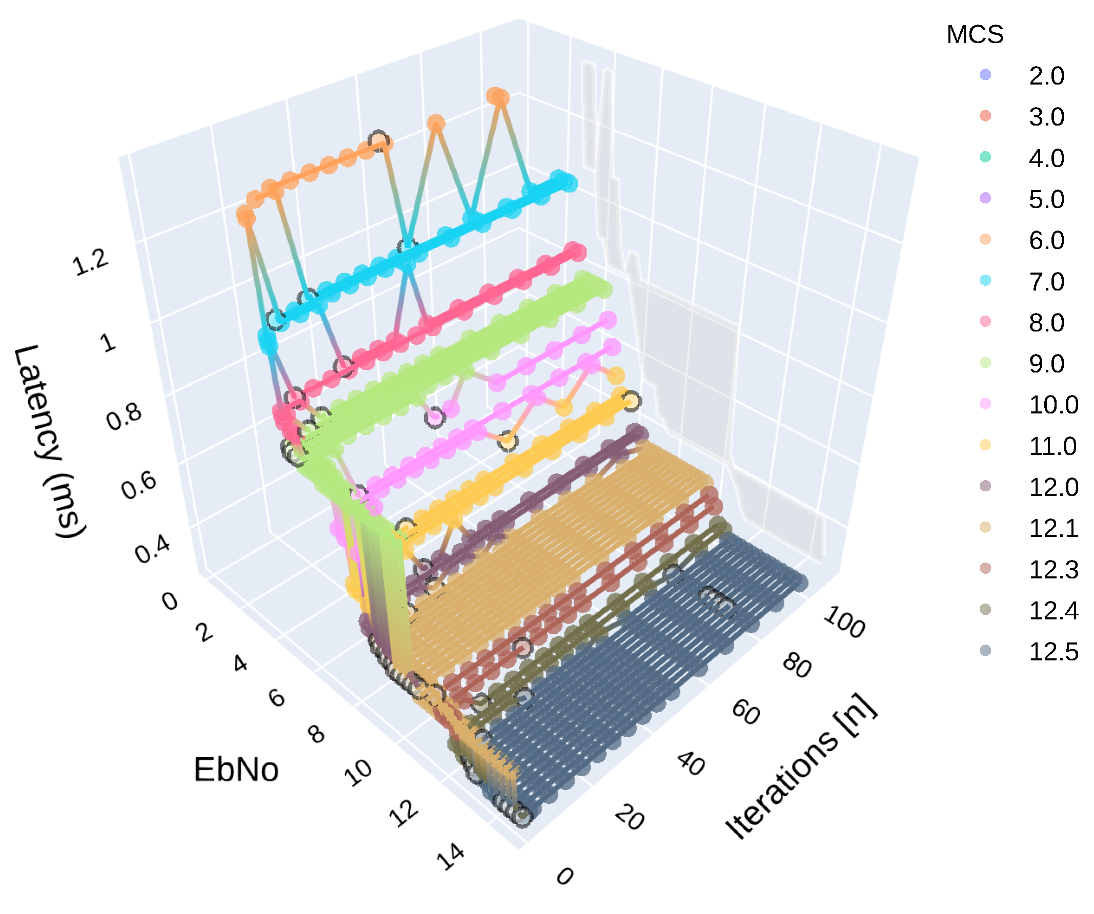
6.1. Allowing More Iterations for Using up Additional Time

Reducing communication latency is of paramount importance for real-time applications; however, when there is additional time available, the PHY can use it for increasing the quality of the received data. An example is adjusting the number of allowed decoding iterations per MCS. Depicted in Figure 14a, every MCS can allow the decoder to execute a given number of iterations before it becomes a bottleneck. For example, allowing it to conduct 20- instead of 10 iterations, during transmission at MCS 2.0, will take up approximately the same amount of time. Beyond that point, the RX can dynamically decide and allow the decoder to consume more time based on the momentary latency constraint. This is especially useful for MCSs with higher indexes, where the decoder becomes a bottleneck at a considerably lower number of iterations. For instance, beyond three iterations for all three of the highest MCS indexes (64QAM). As noted in Section 5.2, making the decoder a bottleneck is not sustainable and is avoided in practice.
Figure 14b illustrates several MCS and E b N 0 combinations where increasing the number of allowed iterations has a considerable effect on the BER. The E b N 0 values are derived from the BER curves in Figure 10a, and they represent the points with the most negative slope. The benefit of executing additional iterations is most visible in those regions of the BER curves. Contrarily, improvements at E b N 0 values with highly erroneous data or with a 0 BER are negligible. These would result in horizontal lines on Figure 14b and have been omitted in view of better visibility of the existing results.
Allowing additional iterations for the MCS— E b N 0 combinations causes a steep decline in BER from 1 to 5 iterations and a moderate improvement in data integrity from 5 to 20 iterations. The observations are further backed by Figure 14c,d. These show a high improvement in terms of BER decrease between 1 and 10 iterations, and somewhat less profitable results when comparing BER values at 10 and 100 iterations. Therefore, selecting the highest possible MCS index that the channel conditions allow will reduce latency, while allowing between 3 and 20 decoding iterations can reduce the amount of erroneous data while sustaining a high enough throughput.

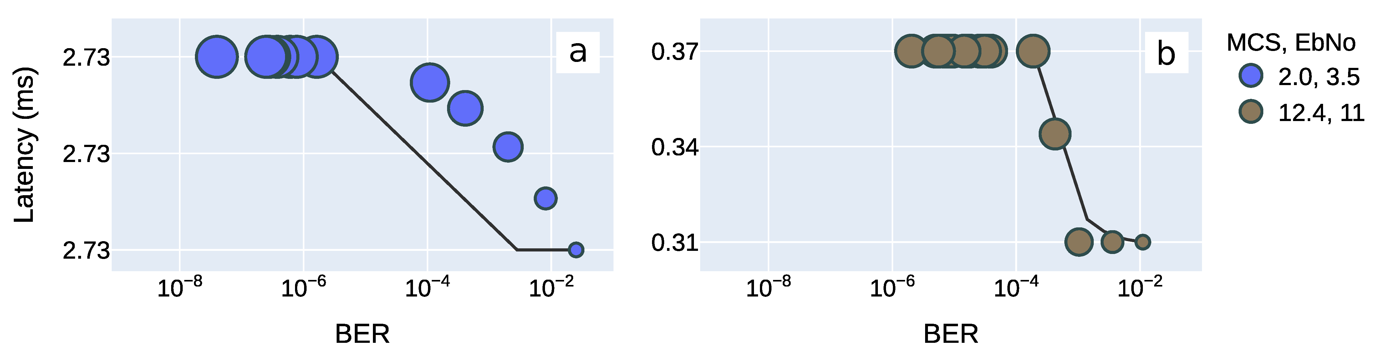
6.2. Latency Versus Bit Error Rate

As mentioned in Section 6.1, latency’s dependency on the BER is most visible in the parts of individual B E R ( E b N 0 ) curves with the steepest negative slope. For example, 3.5- and 11 dB on the two curves associated with MCS 2 and 12.4 in Figure 10a, where every additional decoding iteration will considerably reduce the BER. Figure 15 demonstrates how additional iterations are reflected both in terms of latency and BER; however, the relative change in latency heavily varies between MCSs. In Figure 15a the average number of conducted iterations at MCS 2 varies between 1 and 4.75. The result is a considerable BER reduction, yet, latency only increases by 0.13 µs or 0.005 %. Contrarily, executing between 1 and 3.5 iterations on average at MCS 12.4 will significantly increase latency, illustrated in Figure 15b. The 60 µs (16.2 %) higher latency is a direct consequence of the decoder beginning to act as a bottleneck at more than 3 iterations. The two corner cases show that allowing more decoding iterations at lower MCS indexes significantly reduces BER, while negligibly influencing latency during the reception of 262 kB long payloads. Code rates with less coding overhead benefit less from additional iterations, and MCSs on the other end of the scale can only run a limited amount of decoding iterations before stalling PHY throughput. The horizontally-spread BER values at the highest latency values in Figure 15 are attributed to the stochastic nature of the AWGN channel. The number of incurred iterations is averaged over an entire 262 kB payload, relating to roughly 4000–6000 codewords, depending on the MCS.

6.3. Pareto Optimality

Considering only latency as the optimization metric is often insufficient in practice. A hastily delivered erroneous MPDU might require retransmission, which will further increase the time delay. Hence, applications will in practice impose combined latency and data integrity requirements. Approaching Pareto optimality is achieved by setting the highest allowed BER value and selecting the MCS that generates the least latency. In our case study, the BER limit is set to 10 5 . Decision threshold demapping is used and up to 10 decoding iterations are allowed. The 10 5 threshold value is based on the short packet transmission requirements in 5G NR URLLC. While shorter packets with a 10 5 BER are likely error-free, 262 kB long payloads will on average include 21-bit errors. As reasoned in Section 2.2, the constraint value is kept as a reference since XR video streaming applications are error-tolerant to some extent. Any data points surpassing the BER constraint are discarded; among those in accordance with it, the minimal achieved MPDU latency is extracted. Repeating the process across all E b N 0 values yields a set of minimal latency points, illustrated in Figure 16a. It demonstrates that communication below 3 dB E b N 0 is not feasible when applying the 10 5 BER constraint, marking the point at which a session transfer to a more robust RAT must take place. The remaining points show that single MPDU latency may range from 0.28 to 1.37 ms between 3- and 15 dB.
Figure 16b contains Pareto optimal curves when the constraint and optimization variable are inverted. The curves apply to four distinct maximal PHY latency constraints, and the data points on them represent the proposed MCS for provoking the smallest BER at different noise levels. All BER results converge towards zero beyond a certain E b N 0 value. The curves corresponding to stricter latency constraints are offset towards the right, where noise levels are lower. This is due to the transmission taking place at higher MCS indexes, making it more prone to errors. The two curves corresponding to latency constraints 0.5- and 0.75 ms only exist beyond 5.75- and 6.75 dB. As per to Figure 10c in Section 5.2, the decoder could become a bottleneck at lower E b N 0 values and compromise the latency constraint.
The lowest achievable latency is further evaluated in Figure 17, where the number of allowed decoding iterations is swept from 1 to 100. The data points show considerable similarity to the non-optimized version in Figure 13, except for the results obtained using only a few decoding iterations. Due to the high bit error count at high MCS indexes, these are substituted with their more robust counterparts. Two communicating devices may also agree on the ideal transmission and reception parameters based on momentary channel conditions. The collective approach assumes the RX’ MAC layer has control over the number of PHY LDPC decoding iterations and a parallel communication channel between the two devices exists, avoiding additional time delays. The result is a set of optimal MCS and allowed iteration count combinations, yielding minimal PHY latency. The newly-defined set of points, also outlined in Figure 17, show that switching to a higher indexed MCS at the cost of additional decoding iterations is often beneficial. Most of these switches occur either below 8 dB E b N 0 or at less than 20 decoding iterations. The outliers at 80 iterations and 12–14 dB exist due to an early exit criterion stepping in at fewer executed iterations, far less than the maximal allowed number. The number of allowed iterations can be reduced to reflect the Pareto optimal points below 12- and beyond 14 dB.

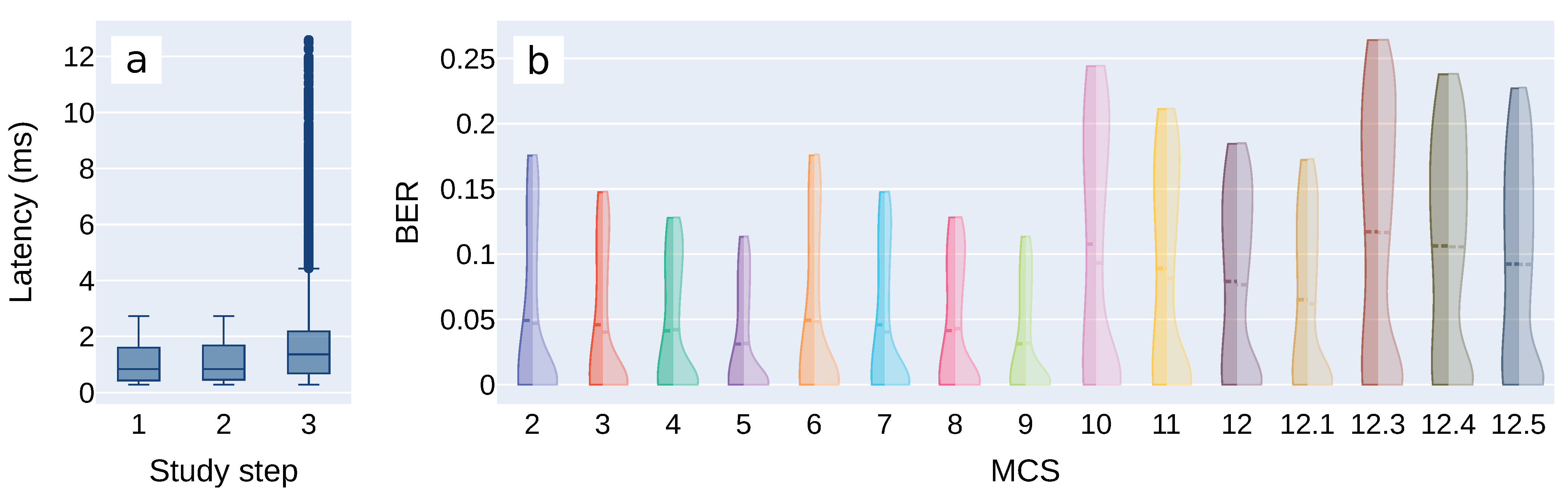
6.4. Summary of Simulation Results

A brief summary of the latency and BER values achieved during individual parts of the study is provided in Figure 18. In accordance with Section 4, steps 1–3 in Figure 18a respectively apply to the ideal case scenario, simulated PHY with 10 allowed decoding iterations, and simulated PHY with 100 allowed decoding iterations. Decision threshold demapping is used in the latter two.
Only minute differences, well below 1 ms, are present between steps 1 and 2. On the other hand, step 3 exhibits far higher latency values with more outliers, which are compensated by the lower achieved BER values. These are presented alongside step 2 BER results in Figure 18b. The higher concentration of BER values towards the bottom of the right part of the distribution plots show how the increase in time is used up for reducing the amount of erroneous data at the RX-side.

7. Conclusions

The present work studies PHY latency in mmWave Wi-Fi networks. It considers both an ideal scenario and a simulated latency-inducing IEEE 802.11ad PHY based on performance figures reported in state-of-the-art literature. Moreover, the simulations include BER results for transmission over an AWGN channel and give insight into individual PHY component data, such as the number of incurred LDPC decoding iterations. The ideal case results show a dependency of the MPDU latency on the employed MCS that grows stronger with the increase in MPDU length. Consequently, the remaining parts of the study focus on the largest allowed payload lengths (262 kB), also emphasizing data-hungry real-time XR applications. Aggregating PPDUs shows a high increase in latency and is discarded during the ideal case study. Evaluating PHY simulation results reveal that latency induced by the RX DBB is highly dependent on the number of incurred decoding iterations, further governed by the amount of noise in the wireless channel. The resulting latency is evaluated for 1–100 decoding iterations, with a closer look at both BER and latency values at 10 and 100 iterations. Three different demapping algorithms—exact, approximative, and decision threshold—are also studied, with the latter yielding the most timely data reception.
In regard to BER, the largest benefits in allowed decoding iteration tuning are identified at 3–20 iterations. The exact tuning region further depends on the available time and the MCS in use. Although the smallest achievable latency values and the MCSs for reaching them are discussed during the evaluation of decoding iterations on latency, the results are revisited in search of Pareto optimality. A set of optimal points is identified in accordance with the 10 5 BER constraint, that generate between 0.28- and 1.37 ms of latency, depending on the selected MCS in Table 2. The lower limit, 0.28 ms, is also the lowest achievable latency during the transmission of 262 kB long payloads. Reducing latency below it would require shortening the payload if the application allows it. In error-intolerant applications, the 10 5 BER constraint may be insufficient and cause retransmission; hence, they would need stricter constraints to avoid generating more latency. In addition to latency-oriented optimization, a group of Pareto curves for generating the least amount of bit errors and complying with four discrete latency constraints is determined. These show the attainable BER regions per latency constraint and can be used in applications emphasizing low-latency operation before reliable data delivery. A final comparison of the studied values is conducted. While latency reduction below that of the ideal case is not possible, parallel MCS and decoder iteration tuning can reduce data loss. These dynamic latency management mechanisms can also work towards lowering the BER by leveraging redundant time when available.
The presented results are all based on 262 kB long PPDU payloads, except for the ideal scenario analysis. The transmission of long sequences inherently takes up a large amount of time, often surpassing the latency generated in the RX DBB. The 2.71 ms latency incurred at MCS index 2—offering the highest reliability—is far from the 1 ms latency constraint imposed by some latency-sensitive applications. Such applications often also feature much shorter payloads. Therefore, more case studies need to be conducted on short payload transmission over WiGig to better understand the relative impact of the RX DBB and to propose adequate latency mitigation mechanisms. Furthermore, transmitting the entire payload using only one of the 15 discussed MCSs results in a limited amount of discrete data transmission latency and reliability outcomes. Splitting the payload in arbitrary lengths and transmitting them at different MCSs could provide fine-grained control over latency and BER.

Author Contributions

Conceptualization, A.M., L.D.S. and L.V.d.P.; Data curation, A.M. and D.D.; Formal analysis, A.M.; Investigation, A.M. and D.D.; Methodology, A.M.; Software, A.M.; Supervision, L.D.S. and L.V.d.P.; Validation, A.M.; Visualization, A.M.; Writing—original draft, A.M., D.D., L.D.S. and L.V.d.P.; Writing—review & editing, A.M., D.D., L.V.d.P. All authors have read and agreed to the published version of the manuscript.

Funding

This work has received funding from the European Union’s Horizon 2020 research and innovation programme under grant agreements: MINTS MSCA-ITN, No 861222; REINDEER RIA, No 101013425.
Electronics 10 01599 i001

Data Availability Statement

The data presented in the manuscript are reproducible using the simulation framework, found at https://github.com/PhyPy-802dot11ad (accessed on 31 May 2021).

Conflicts of Interest

The authors declare no conflict of interest.

References

  1. Cisco and Its Affiliates. Cisco Annual Internet Report (2018–2023). 2020. Available online: https://www.cisco.com/c/en/us/solutions/collateral/executive-perspectives/annual-internet-report/white-paper-c11-741490.html (accessed on 14 May 2021).
  2. IEEE Computer Society. Directional multi-gigabit (DMG) PHY specification. In 802.11-2016—IEEE Standard for Information Technology—Telecommunications and Information Exchange between Systems Local and Metropolitan area Networks—Specific Requirements—Part 11: Wireless LAN Medium Access Control (MAC) and Physical Layer (PHY) Specifications; IEEE: New York, NY, USA, 2016; pp. 2436–2496. ISBN 9781504436458. [Google Scholar] [CrossRef]
  3. IEEE Communications Society. Very high throughput (VHT) PHY specification. In IEEE Standard for Information Technology—Telecommunications and Information Exchange between Systems Local and Metropolitan Area Networks—Specific Requirements—Part 11: Wireless LAN Medium Access Control (MAC) and Physical Layer (PHY) Specifications; IEEE: New York, NY, USA, 2016; pp. 2497–2624. ISBN 9781504436458. [Google Scholar] [CrossRef]
  4. Yao, R.; Heath, T.; Davies, A.; Forsyth, T.; Mitchell, N.; Hoberman, P. Oculus VR Best Practices Guide; Technical Report 36.777; Oculus VR Inc.: Irvine, CA, USA, 2014; Version 0.008. [Google Scholar]
  5. Adame, T.; Carrascosa, M.; Bellalta, B. Time-Sensitive Networking in IEEE 802.11be: On the Way to Low-latency WiFi 7. arXiv 2019, arXiv:1912.06086. [Google Scholar]
  6. 3GPP. Study on Communication for Automation in Vertical Domains; Technical Report (TR) 22.804; 3rd Generation Partnership Project (3GPP): Sophia Antipolis, France, 2020; Version 16.3.0. [Google Scholar]
  7. Siddiqi, M.A.; Yu, H.; Joung, J. 5G Ultra-Reliable Low-Latency Communication Implementation Challenges and Operational Issues with IoT Devices. Electronics 2019, 8, 981. [Google Scholar] [CrossRef] [Green Version]
  8. Kanavos, A.; Fragkos, D.; Kaloxylos, A. V2X Communication over Cellular Networks: Capabilities and Challenges. Telecom 2021, 2, 1. [Google Scholar] [CrossRef]
  9. Kim, C.; Tomas Gareau, N.M. 5G for Drone-Based Vertical Applications—D1.1 Use Case Specifications and Requirements; Technical Report; 5G!Drones: Oulu, Finland, 2019; Version 1.0. [Google Scholar]
  10. 5GACIA. 5G for Connected Industries and Automation; Technical Report; 5G Alliance for Connected Industries and Automation (5GACIA): Frankfurt, Germany, 2019. [Google Scholar]
  11. Elbamby, M.S.; Perfecto, C.; Bennis, M.; Doppler, K. Toward Low-Latency and Ultra-Reliable Virtual Reality. IEEE Netw. 2018, 32, 78–84. [Google Scholar] [CrossRef] [Green Version]
  12. Singh, H.; Oh, J.; Kweon, C.; Qin, X.; Shao, H.R.; Ngo, C. A 60 GHz wireless network for enabling uncompressed video communication. IEEE Commun. Mag. 2008, 46, 71–78. [Google Scholar] [CrossRef]
  13. Furst, J.; Argerich, M.F.; Cheng, B.; Papageorgiou, A. Elastic Services for Edge Computing; Poster Session; IEEE: Rome, Italy, 2018; p. 5. [Google Scholar]
  14. Bailey, R.E.; Parrish, R.V.; Arthur III, J.J.; Norman, R.M. Latency Requirements for Head-Worn Display S/EVS Applications; SPIE, Enhanced and Synthetic Vision: Orlando, FL, USA, 2004; Volume 5424, pp. 98–109. [Google Scholar] [CrossRef] [Green Version]
  15. Jerald, J.; Whitton, M. Relating Scene-Motion Thresholds to Latency Thresholds for Head-Mounted Displays. In Proceedings of the IEEE Virtual Reality Conference, Lafayette, LA, USA, 14–18 March 2009; pp. 211–218. [Google Scholar] [CrossRef] [Green Version]
  16. Geršak, G.; Lu, H.; Guna, J. Effect of VR technology matureness on VR sickness. Multimed. Tools Appl. 2020, 79, 14491–14507. [Google Scholar] [CrossRef]
  17. Potter, M.C.; Wyble, B.; Hagmann, C.E.; McCourt, E.S. Detecting meaning in RSVP at 13 ms per picture. Atten. Percept. Psychophys. 2014, 76, 270–279. [Google Scholar] [CrossRef] [PubMed] [Green Version]
  18. Shukla, G.; Beg, M.T.; Lall, B. Evaluation of Latency in IEEE 802.11ad. In Innovations in Electronics and Communication Engineering; Series Title: Lecture Notes in Networks and Systems; Saini, H.S., Singh, R.K., Tariq Beg, M., Sahambi, J.S., Eds.; Springer: Singapore, 2020; Volume 107, pp. 139–145. [Google Scholar] [CrossRef]
  19. Wei, T.; Zhang, X. Pose Information Assisted 60 GHz Networks: Towards Seamless Coverage and Mobility Support. In Proceedings of the 23rd Annual International Conference on Mobile Computing and Networking, Snowbird, UT, USA, 16–20 October 2017; pp. 42–55. [Google Scholar] [CrossRef]
  20. Kim, S.; Yun, J.H. Motion-Aware Interplay between WiGig and WiFi for Wireless Virtual Reality. Sensors 2020, 20, 6782. [Google Scholar] [CrossRef]
  21. Liu, L.; Zhong, R.; Zhang, W.; Liu, Y.; Zhang, J.; Zhang, L.; Gruteser, M. Cutting the Cord: Designing a High-quality Untethered VR System with Low Latency Remote Rendering. In Proceedings of the 16th Annual International Conference on Mobile Systems, Applications, and Services, Munich, Germany, 10–15 June 2018; pp. 68–80. [Google Scholar] [CrossRef]
  22. Ravichandran, A.; Jain, I.K.; Hegazy, R.; Wei, T.; Bharadia, D. Facilitating Low Latency and Reliable VR over Heterogeneous Wireless Networks. In Proceedings of the 24th Annual International Conference on Mobile Computing and Networking, New Delhi, India, 29 October–2 November 2018; pp. 723–725. [Google Scholar] [CrossRef]
  23. Sur, S.; Pefkianakis, I.; Zhang, X.; Kim, K.H. WiFi-Assisted 60 GHz Wireless Networks. In Proceedings of the 23rd Annual International Conference on Mobile Computing and Networking, Snowbird, UT, USA, 16–20 October 2017; pp. 28–41. [Google Scholar] [CrossRef]
  24. Lu, C.; Wu, B.; Wang, L.; Wei, Z.; Tang, Y. A Novel QoS-Aware ARQ Scheme for Multi-User Transmissions in IEEE802.11ax WLANs. Electronics 2020, 9, 2065. [Google Scholar] [CrossRef]
  25. Lu, C.; Wu, B.; Ye, T. A Novel QoS-Aware A-MPDU Aggregation Scheduler for Unsaturated IEEE802.11n/ac WLANs. Electronics 2020, 9, 1203. [Google Scholar] [CrossRef]
  26. Shah, V.; Cooklev, T. Throughput and latency performance of IEEE 802.11e with 802.11a, 802.11b, and 802.11g physical layers. J. Inst. Eng. India Ser. B 2004, 93, 247–253. [Google Scholar] [CrossRef]
  27. Jiang, X.; Shokri-Ghadikolaei, H.; Fodor, G.; Modiano, E.; Pang, Z.; Zorzi, M.; Fischione, C. Low-Latency Networking: Where Latency Lurks and How to Tame It. Proc. IEEE 2019, 107, 280–306. [Google Scholar] [CrossRef]
  28. Fehrenbach, T.; Datta, R.; Göktepe, B.; Wirth, T.; Hellge, C. URLLC Services in 5G Low Latency Enhancements for LTE. In Proceedings of the 2018 IEEE 88th Vehicular Technology Conference (VTC-Fall), Chicago, IL, USA, 27–30 August 2018; pp. 1–6. [Google Scholar] [CrossRef] [Green Version]
  29. Ji, H.; Park, S.; Yeo, J.; Kim, Y.; Lee, J.; Shim, B. Ultra-Reliable and Low-Latency Communications in 5G Downlink: Physical Layer Aspects. IEEE Wirel. Commun. 2018, 25, 124–130. [Google Scholar] [CrossRef] [Green Version]
  30. Sachs, J.; Wikstrom, G.; Dudda, T.; Baldemair, R.; Kittichokechai, K. 5G Radio Network Design for Ultra-Reliable Low-Latency Communication. IEEE Netw. 2018, 32, 24–31. [Google Scholar] [CrossRef]
  31. Jung, Y.M.; Chung, C.H.; Jung, Y.H.; Kim, J.S. 7.7 Gbps Encoder Design for IEEE 802.11ac QC-LDPC Codes. In Proceedings of the 2012 International SoC Design Conference (ISOCC), Jeju, South Korea, 4–7 November 2012. [Google Scholar]
  32. Genc, Z.; Thillo, W.V.; Bourdoux, A.; Onur, E. 60 GHz PHY Performance Evaluation with 3D Ray Tracing under Human Shadowing. IEEE Wirel. Commun. Lett. 2012, 1, 117–120. [Google Scholar] [CrossRef]
  33. Chen, J.; Lin, H.; Tang, Y.C. Efficient high-throughput architectures for high-speed parallel scramblers. In Proceedings of the IEEE International Symposium on Circuits and Systems (ISCAS), Paris, France, 30 May–2 June 2010; pp. 441–444. [Google Scholar] [CrossRef]
  34. Budišin, S. Efficient pulse compressor for golay complementary sequences. Electron. Lett. 1991, 27, 219. [Google Scholar] [CrossRef]
  35. Ahmed, T.; Garrido, M.; Gustafsson, O. A 512-point 8-parallel pipelined feedforward FFT for WPAN. In Proceedings of the 2011 Conference Record of the Forty Fifth Asilomar Conference on Signals, Systems and Computers (ASILOMAR), Pacific Grove, CA, USA, 6–9 November 2011; pp. 981–984. [Google Scholar] [CrossRef] [Green Version]
  36. Jafri, A.R.; Baghdadi, A.; Waqas, M.; Najam-Ul-Islam, M. High-Throughput and Area-Efficient Rotated and Cyclic Q Delayed Constellations Demapper for Future Wireless Standards. IEEE Access 2017, 5, 3077–3084. [Google Scholar] [CrossRef]
  37. Jafri, A.; Baghdadi, A.; Jezequel, M. ASIP-Based Universal Demapper for Multiwireless Standards. IEEE Embed. Syst. Lett. 2009, 1, 9–13. [Google Scholar] [CrossRef]
  38. Ali, I.; Wasenmüller, U.; Wehn, N. A high throughput architecture for a low complexity soft-output demapping algorithm. Adv. Radio Sci. 2015, 13, 73–80. [Google Scholar] [CrossRef] [Green Version]
  39. Kuon, I.; Rose, J. Measuring the Gap Between FPGAs and ASICs. IEEE Trans. Comput. Aided Des. Integr. Circuits Syst. 2007, 26, 203–215. [Google Scholar] [CrossRef] [Green Version]
  40. Borkar, S. Design challenges of technology scaling. IEEE Micro 1999, 19, 23–29. [Google Scholar] [CrossRef]
  41. Stillmaker, A.; Baas, B. Scaling equations for the accurate prediction of CMOS device performance from 180 nm to 7 nm. Integration 2017, 58, 74–81. [Google Scholar] [CrossRef]
  42. Salbiyono, A.; Adiono, T. LDPC decoder performance under different number of iterations in mobile WiMax. In Proceedings of the 2010 International Symposium on Intelligent Signal Processing and Communication Systems, Chengdu, China, 6–8 December 2010; pp. 1–4. [Google Scholar] [CrossRef]
  43. Koike-Akino, T.; Millar, D.S.; Kojima, K.; Parsons, K.; Miyata, Y.; Sugihara, K.; Matsumoto, W. Iteration-Aware LDPC Code Design for Low-Power Optical Communications. J. Light. Technol. 2016, 34, 573–581. [Google Scholar] [CrossRef]
  44. Li, M.; Naessens, F.; Li, M.; Debacker, P.; Desset, C.; Raghavan, P.; Dejonghe, A.; Van der Perre, L. A processor based multi-standard low-power LDPC engine for multi-Gbps wireless communication. In Proceedings of the 2013 IEEE Global Conference on Signal and Information Processing, Austin, TX, USA, 3–5 December 2013; pp. 1254–1257. [Google Scholar] [CrossRef]
  45. Marinšek, A.; Van der Perre, L. Keeping up with the Bits: Tracking Physical Layer Latency in Millimeter-Wave Wi-Fi Networks. arXiv 2021, arXiv:cs.NI/2105.13147. [Google Scholar]
  46. Franceschini, M.; Ferrari, G.; Raheli, R. Decoding algorithms for LDPC codes. In LDPC Coded Modulations; Signals and Communication Technology; Springer: Berlin/Heidelberg, Germany, 2009; pp. 42–53. [Google Scholar] [CrossRef]
  47. Borlenghi, F.; Witte, E.M.; Ascheid, G.; Meyr, H.; Burg, A. A 772Mbit/s 8.81bit/nJ 90nm CMOS soft-input soft-output sphere decoder. In Proceedings of the IEEE Asian Solid-State Circuits Conference, Jeju, Korea, 14–16 November 2011; pp. 297–300. [Google Scholar] [CrossRef]
Figure 1. Observed latency: from an MPDU entering the PHY at the TX to its hand-off between the RX’ PHY and MAC layer.
Electronics 10 01599 g001
Figure 2. Schematic view of a PPDU, including aggregated PPDUs.
Electronics 10 01599 g002
Figure 3. IEEE 802.11ad PHY receiver digital baseband. Above each component lies its input buffer with the corresponding base unit size noted on its left. Solid connections show data propagation paths, while dashed lines correspond to flag indicators. The processing operations contributing to latency beyond the finite symbol rate are written in bold. Those with additional control over the inflicted latency are colored in blue.
Electronics 10 01599 g003
Figure 4. Component time delay performance figures, illustrated on an example.
Electronics 10 01599 g004
Figure 5. Task execution flow in the channel and noise estimation block. Vertical task stacking represents parallel execution.
Electronics 10 01599 g005
Figure 6. Two-part error and latency simulation framework. Blocks with a dashed outline change depending on the study step, while the number of decoder iterations is passed on between the two parts.
Electronics 10 01599 g006
Figure 7. Difference between the blocks in the bit error simulation process, dependent on the study step.
Electronics 10 01599 g007
Figure 8. Dependence of the first latency probing simulation block on the study step.
Electronics 10 01599 g008
Figure 9. From left to right: latency’s dependency on the MCS and payload length (a); Increase in latency per each additional kB of data, dependent on the MCS (b). White curves represent latency isohypses.
Electronics 10 01599 g009
Figure 10. Counterclockwise from top left: incurred BER during transmission (a); average number of executed decoding iterations (b); resulting MPDU latency (c). Obtained using the decision threshold demapper and allowing up to 10 LDPC decoding iterations. The dashed line in (a) represents the 10 5 BER limit, as defined by 5G NR.
Electronics 10 01599 g010
Figure 11. MPDU latency for exact, approximative, and decision threshold demapping. The maximum number of decoding iterations is 10.
Electronics 10 01599 g011
Figure 12. From left to right: incurred MPDU latency (a) and BER (b) when setting the largest allowed number of LDPC decoding iterations to 100. MCS colour codes are the same as in previous figures. The white region on the left subplot represents the expected latency region, governed by MCS and E b N 0 .
Electronics 10 01599 g012
Figure 13. Minimal achievable latency at different channel noise levels and maximum allowed number of LDPC decoding iterations. The colour represents the MCS at which minimal latency was achieved.
Electronics 10 01599 g013
Figure 14. From the top down and left to right: incurred latency when increasing the number of allowed decoding iterations (a); resulting BER for given MCS and E b N 0 combinations—the latter is represented by line width (b); BER difference when comparing 1- to 10- (c) and 10- to 100 decoding iterations (d).
Electronics 10 01599 g014
Figure 15. Trade-off between latency and BER at two distinct MCS and E b N 0 combinations. Marker size represents the average number of incurred iterations, ranging from 1 to 4.75. The grey curve represents a reference 1 x function fitted to the data points. Both Y-axes are rounded to two decimal points. The 0.13 µs MCS 2 latency difference from top to bottom is contained within the roundoff.
Electronics 10 01599 g015
Figure 16. From left to right: Pareto optimal latency points with regard to the 10 5 BER constraint; Pareto optimal curves for achieving minimal BER at different maximal latency constraints. Colours represent the MCS at which the Pareto optimal points are achieved.
Electronics 10 01599 g016
Figure 17. Selection of points with minimal latency that satisfy the 10 5 BER constraint. Colours represent the MCS at which the Pareto optimal points are achieved, the expected latency region is highlighted by the white polygon on the back plane, and iteration-independent optimal points are circled in grey.
Electronics 10 01599 g017
Figure 18. Left to right: comparison of expected latency regions (a); BER comparison for the two PHY simulation cases (b), with the left and right parts of the distributions corresponding to study steps 2 and 3, respectively.
Electronics 10 01599 g018
Table 1. Use cases imposing strict latency constraints.
IndustryApplicationMax. Latency (ms)Latency TypeRef.
XRVR entertainment20RTT and E2E[4,5]
Professional AR/MR usage10RTT and E2E[6,7]
V2X, UVsPlatooning25RTT[6,8,9]
andRemote control10E2E[6,7,8,9]
dronesCooperative driving/flight10RTT[6,7,8,9]
i4.0Remote control and monitoring50E2E[10]
Cooperative robots1RTT[10]
Table 2. MCSs associated with different modulation and code rates.
BPSKQPSK16QAM64QAM
1 2 2610/
5 8 371112.3
3 4 481212.4
13 16 5912.112.5
Table 3. Throughput performance metrics and demapping algorithms associated with the three different demapper instances. The throughput applies to five parallel demappers, as described in the corresponding references. All throughput values and the set of demapping equations in the last row correspond to 16QAM mapping.
NameThroughput ( MLLR s )Demapping AlgorithmRef.
Exact800 L L R [ k ] = l n i = 0 2 M 1 e x p ( 1 2 σ 2 · r c i , 1 2 ) i = 0 2 M 1 e x p ( 1 2 σ 2 · r c i , 0 2 ) [36]
Approximative3030 L L R [ k ] = 1 2 σ 2 · [ min ( r c i , 0 2 ) min ( r c i , 1 2 ) ] [37]
Decision threshold6640 L L R [ 0 ] = 1 2 σ 2 · Re ( r )
L L R [ 1 ] = 1 2 σ 2 · ( 2 | Re ( r ) | )
L L R [ 2 ] = 1 2 σ 2 · Im ( r )
L L R [ 3 ] = 1 2 σ 2 · ( 2 | Im ( r ) | )
[38]
Table 4. Total MPDU latency without aggregation (0) and when appending a single A-PPDU (1), per MCS index. All values are in milliseconds.
A-PPDU2345678910111212.112.312.412.5
02.732.181.821.681.361.090.910.840.680.550.460.420.370.310.28
15.454.363.633.362.732.181.821.681.371.090.910.840.730.610.56
Publisher’s Note: MDPI stays neutral with regard to jurisdictional claims in published maps and institutional affiliations.

