Efficient Binarized Convolutional Layers for Visual Inspection Applications on Resource-Limited FPGAs and ASICs

Abstract

There has been a recent surge in publications related to binarized neural networks (BNNs), which use binary values to represent both the weights and activations in deep neural networks (DNNs). Due to the bitwise nature of BNNs, there have been many efforts to implement BNNs on ASICs and FPGAs. While BNNs are excellent candidates for these kinds of resource-limited systems, most implementations still require very large FPGAs or CPU-FPGA co-processing systems. Our work focuses on reducing the computational cost of BNNs even further, making them more efficient to implement on FPGAs. We target embedded visual inspection tasks, like quality inspection sorting on manufactured parts and agricultural produce sorting. We propose a new binarized convolutional layer, called the neural jet features layer, that learns well-known classic computer vision kernels that are efficient to calculate as a group. We show that on visual inspection tasks, neural jet features perform comparably to standard BNN convolutional layers while using less computational resources. We also show that neural jet features tend to be more stable than BNN convolution layers when training small models.

1. Introduction

Deep learning (DL) models currently dominate as the state-of-the-art method for image classification tasks. They are versatile and achieve unprecedented accuracy for most applications. Unlike traditional computer vision approaches, DL can construct complex models with little to no expert knowledge of the target domain.

DL models tend to be large and computationally intensive. They are well suited for complex image classification tasks, but many straightforward image classification applications do not require such complexity, but could still benefit from the ease of use that DL provides. Many applications, like quality inspection in manufacturing and agricultural produce sorting, rely on automated image classification systems, but do not require overly complex DL models. Instead, they benefit from systems that are high-speed, low-cost, low-power and small form-factor. FPGAs and ASICs make great candidates for these types of applications, but generally lack the computational resources to run mainstream DL models at reasonable speeds.

In this work, we propose a new binarized convolutional layer called the neural jet features layer. The neural jet features layer is a convolutional layer that is trained to form jet features within a BNN using DL methods. This creates a BNN model that is less costly to compute on resource-limited systems while maintaining comparable classification accuracy. We also show that neural jet features are more stable during training on the MNIST dataset.

Related Work

Various efforts have been made to make deep neural networks (DNNs) less resource intensive. Models like SqueezeNet [1] and techniques like network pruning [2,3,4] are effective ways to reduce the number of operations required by a NN. They do not reduce the complexity of those operations. GhostNET [5] reduces the number of convolutional operations needed in a convolutional layer by generating fewer feature maps. These feature maps are then augmented by applying various linear operations to each of these intrinsic feature maps, creating more features with fewer convolution operations. Our work shares a similar philosophy by reusing feature maps between different output channels, as explained in Section 3.2.

Quantized neural networks use low-precision fixed-point values instead of full-precision floating-point values, making the operations of the network simpler and more compatible with limited resource systems. Binarized neural networks (BNNs) use the most extreme form of network quantization, using single bits to represent values throughout the model. The original BNN model, as proposed by Courbariaux et al. [6], was shown to perform well on simple image classification tasks like MNIST and CIFAR-10, but was not well suited for the ImageNet [7] dataset. Many subsequent works have augmented BNNs to perform better on ImageNet at the cost of greater network complexity and larger model size. The larger models usually require very large FPGAs and/or CPU co-processors [8]. In this work, instead of making BNNs more complex, we seek to reduce the size of BNNs while maintaining comparable accuracy for simpler image classification tasks, which can be implemented in resources-limited FPGAs and ASICs. FPGAs and ASICs tend to be much less power-hungry than GPUs and CPUs on quantized and binarized values. Qasaimeh et al. [9] have shown that on floating-point arithmetic image processing tasks, FPGAs, CPUs, and GPUs consume similar amounts of power. However, FPGAs are not well equipped to process floating-point values like CPUs and GPUs. On image processing pipelines that used quantized values, FPGAs consume $10\times$ to $20\times$ less power.

In our previous work, we presented jet features [10], a set of convolution kernels that are efficient to compute on resource-limited systems, which utilize the key scaling and partial derivative properties of classic image processing kernels. We demonstrated their effectiveness by replacing the set of traditional image features used in the ECO features algorithm [11] with jet features, which allowed the algorithm to be effectively implemented on an FPGA for high-speed, low-power classification without sacrificing image classification accuracy.

2. Background

2.1. Binarized Neural Networks

BNN are deep neural networks that use binarized values (−1 and 1) for their weights and activations. BNNs were first introduced by Courbariaux et al. [6], and the methods they introduced are still the most widely used form of network binarization.

Courbariaux et al. first presented a method for binarizing the weights of DNNs known as BinaryConnect [12]. This was the first known technique to directly train binary values in a DNN, which is not possible with standard deep learning methods. Standard deep learning uses gradient descent, which makes incremental changes to a model’s weights, which is not possible with binary valued weights. To overcome this challenge, BinaryConnect trains set of full-precision weights, which can be updated in small increments, but passes these weights through a binarization layer before being used by the network, as show in Figure 1.

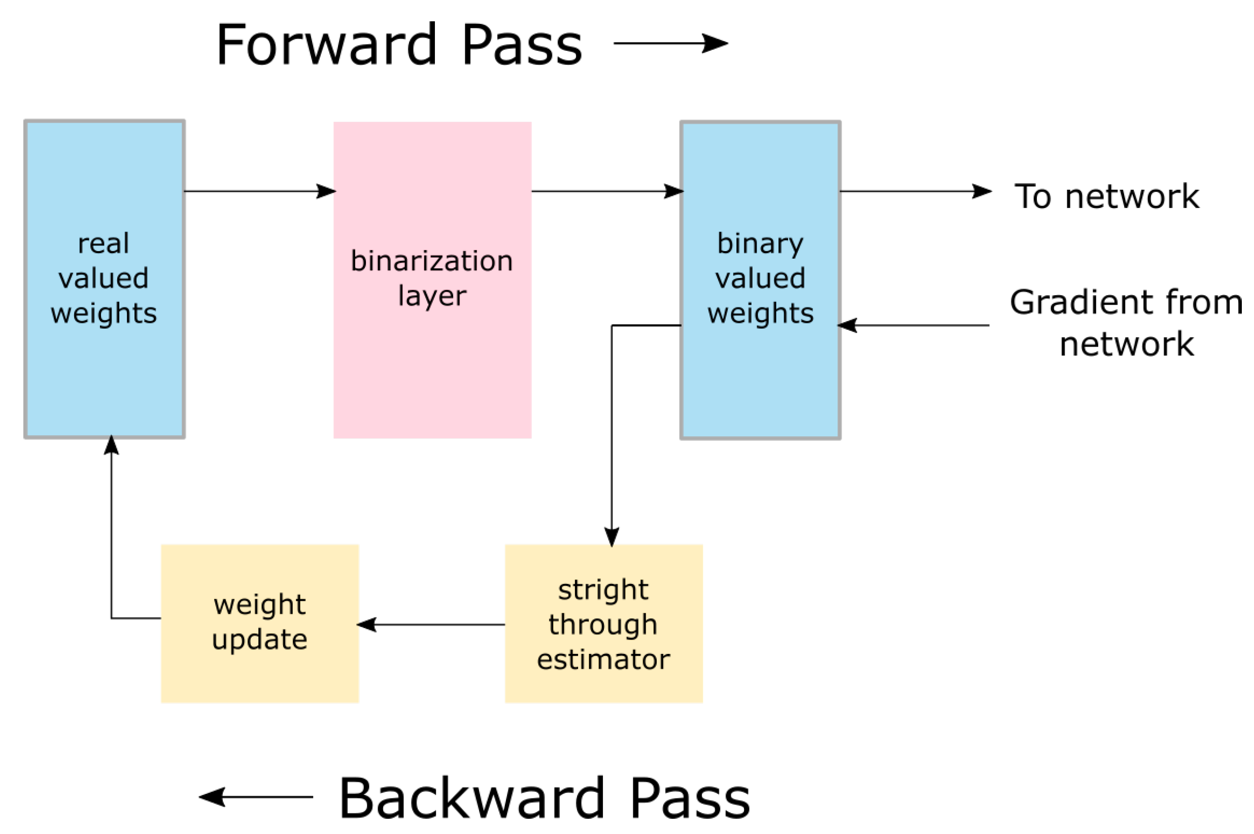
2.1.1. Binarization of Weights

The binarization layer produces a binary output by taking the sign of its input (−1 or 1). Standard backpropagation with a discrete function, like the sign function, produces a gradient of zero, which is incompatible with gradient decent. Instead of using standard backpropagation, the binarization layer uses a Straight Through Estimator (STE) [13]. The STE ignores the sign function during backpropagation and passes the gradient at the output of the layer through to the input of the layer, as shown in Figure 1. This allows for the real-valued background weights to be updated during the backward pass while the binary valued weights are used during the forward pass. Once training is complete, the real valued background weights are no longer needed.

With binary valued weights, BinaryConnect reduces the model size of the network and lowers the computational cost of the operations. Instead of multiplying two floating-point values, the signs of activation are merely flipped according to the binary valued weights, which requires no multiplication operations at all. Courbariaux et al. were able to show that binary connect could match the accuracy of contemporary full precision methods on the MNIST, CIFAR-10 and SVHN datasets.

2.1.2. Binarization of Activations

After BinaryConnect showed that directly training binary valued weights was feasible, Courbariaux et al. developed the BNN model, which uses binary values for both weights and activations. This reduces computational cost even further. By encoding values of −1 as 0 and +1 as 1, weights can be applied to activations through bitwise XNOR logic operations. The single bit results can then be accumulated with simple bit counting operations.

In order to binarize activations, BNNs pass the activations through the same STE binarization layers that are used to binarize the weights. Courbariaux et al. noticed that as gradients are backpropagated through multiple binarized layers, they encounter many activations exceeding an absolute value of 1. This causes the gradients to grow rapidly and explode. To counteract this, BNNs artificially force the gradients to zero whenever they pass through layers whose activations have an absolute value greater than 1.

2.1.3. Performance and Improvements

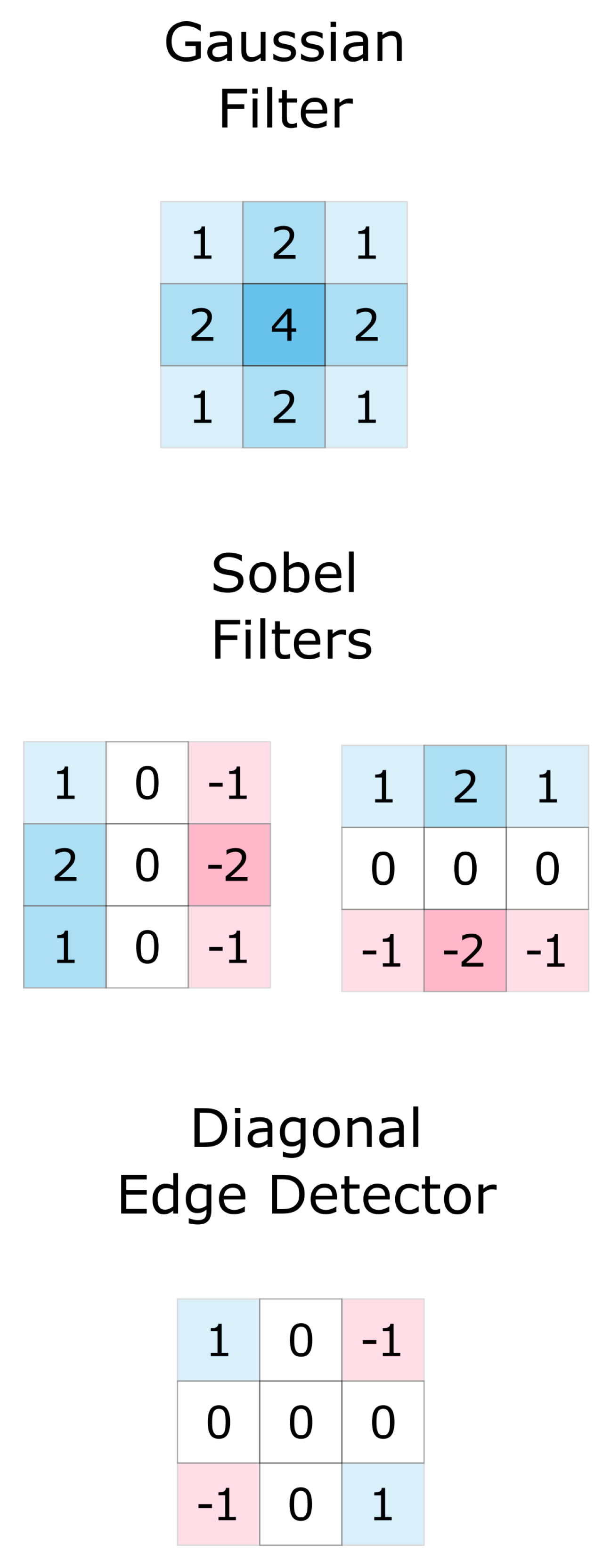
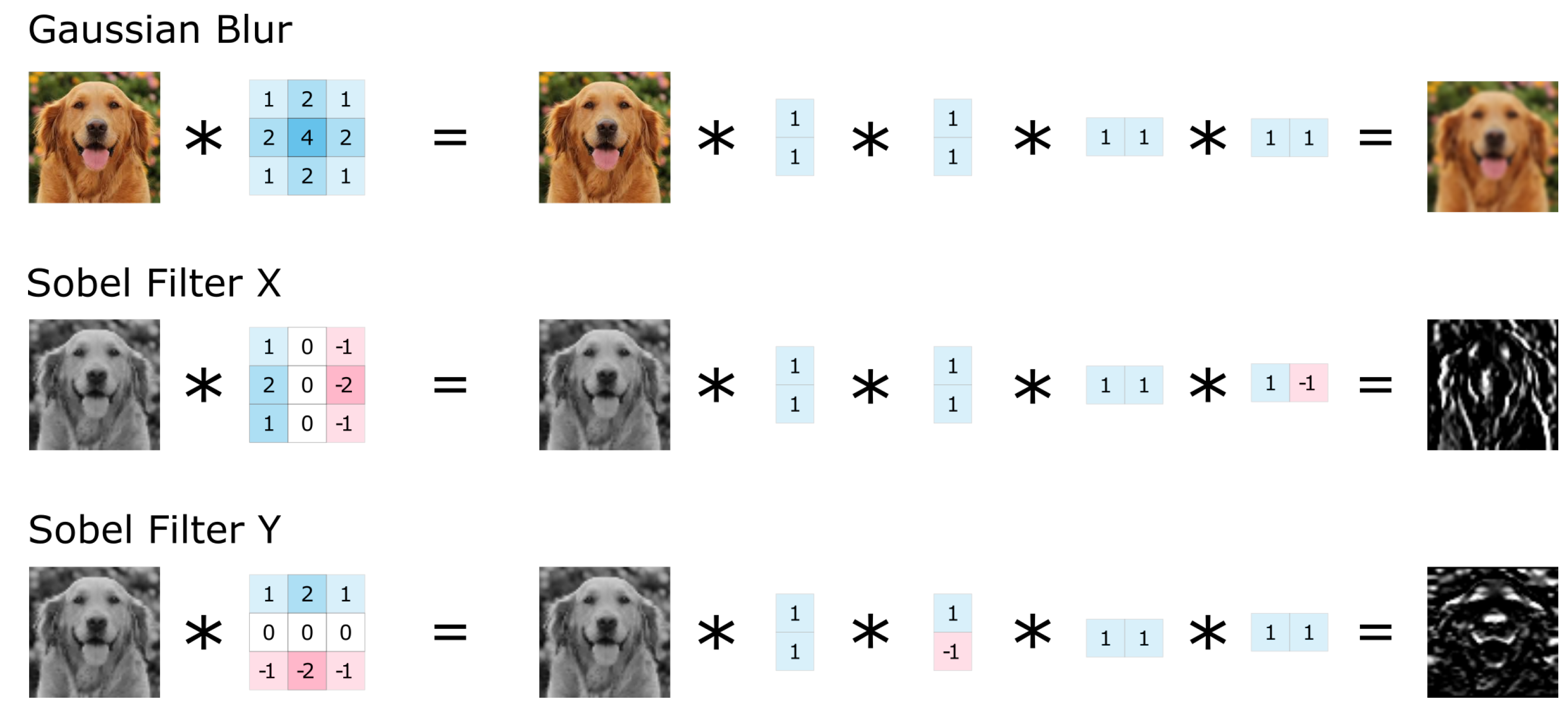
Courbariaux et al. reported that on simple datasets like MNIST and CIFAR-10, BNNs could achieve comparable accuracy to their full precision counter parts, but failed to produce similar success on the more complex ImageNet dataset. Various efforts have been made to improve performance on more complex image classification datasets. Rastegari et al. proposed XNOR-Net, which is similar to the original BNN, but augments the model with some full-precision calculations to more faithfully match full-precision models [14]. Zhou et al. generalized quantized networks with the DoReFa model which broke down full-precision arithmetic into bitwise operations [15]. ABC-Net, developed by Lin et al., used learned scaling factors and multiple parallel binarization layers to add capacity and complexity to BNNs. These efforts led to increased accuracy on the ImageNet dataset, but significantly increased the number and/or complexity of operations required within the model [16].

2.2. Jet Features

Additional research has focused on implementing BNNs on efficient platforms like ASICs, FPGAs and FPGA-CPU hybrid systems. Some works have focused on binarizing even more aspects of the BNN model. Several works have noticed that previous BNNs used zeros to pad the inputs to convolutional layers, which were not a part of the binary set of value −1 and 1 [17,18,19]. Multiple works have focused on designing BNN accelerators, especially useful in CPU-FPGA designs [17,18,20,21]. Other works have focused on stand-alone streaming models for very high-speed image classification. While many works have reported success in implementing BNNs in FPGA for task like MNIST and CIFAR-10 image classification, they generally require a large FPGA, like the Xilinx Vertex or Kintex UltraScale, or they employ a CPU-FPGA hybrid systems [8] like the Xilinx Zynq MPSoC. In this work, we are interested in making BNNs even more efficient by reducing the computational cost of convolution operations, allowing them to be implemented in small to midsize FPGAs for affordable high-speed classification on low power and portable platforms.

In our previous work, we introduced the concept of jet features [10], which are a set of convolutional kernels that are especially efficient to compute as a group. They take advantage of the core elements of popular image processing kernels like the Gaussian and Sobel kernels. These features were originally developed to replace the traditional image processing transforms that was used in the ECO feature algorithm [22].

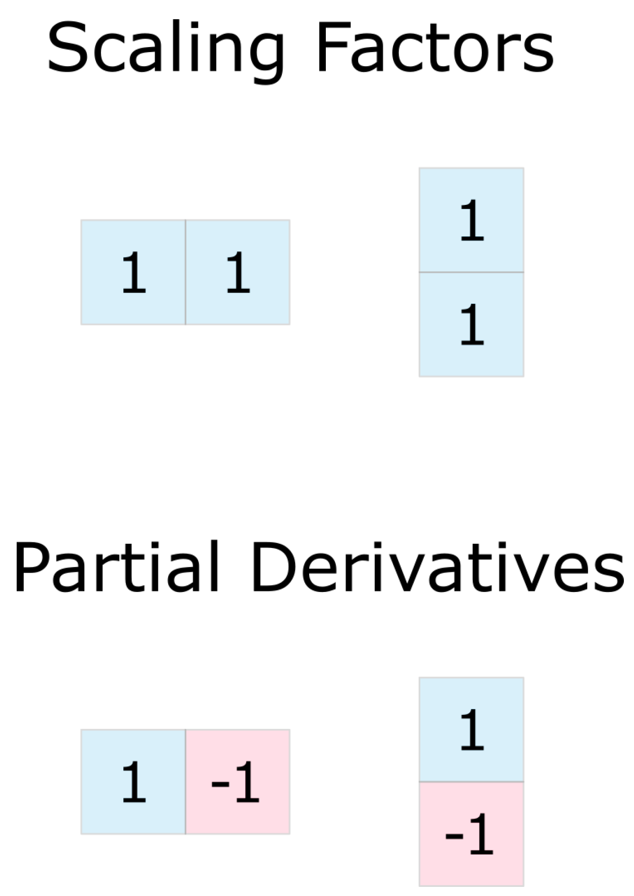
2.2.1. Definition of Jet Features

Jet features are convolution kernels that can be broken down into a series of smaller convolutions with special $2\times 1$ kernels chosen from the set [1, 1], [1, −1], [1, 1]${|}^T$, [1, −1]${}^T$. Examples of a few jet features are shown in Figure 2. Convolutions with these small kernels either takes the sum or difference of adjacent pixels, in either the vertical or horizontal direction. Taking the sum of adjacent pixels blurs the image, which effectively scales the input image [22]. Taking the difference of adjacent pixels produces a partial derivative, useful for gradient calculation. For this reason, we refer to these small kernels as scaling factors and partial derivatives, as shown in Figure 3.

Traditional computer vision algorithms make heavy use of scaling operations and derivative calculation [22,23]. The most popular image processing kernels, like the Sobel, Gaussian and Laplacian filters, can be duplicated or approximated from a series of these scaling factors and partial derivatives. Figure 4 shows how the Sobel and Gaussian kernels can be duplicated from these building blocks.

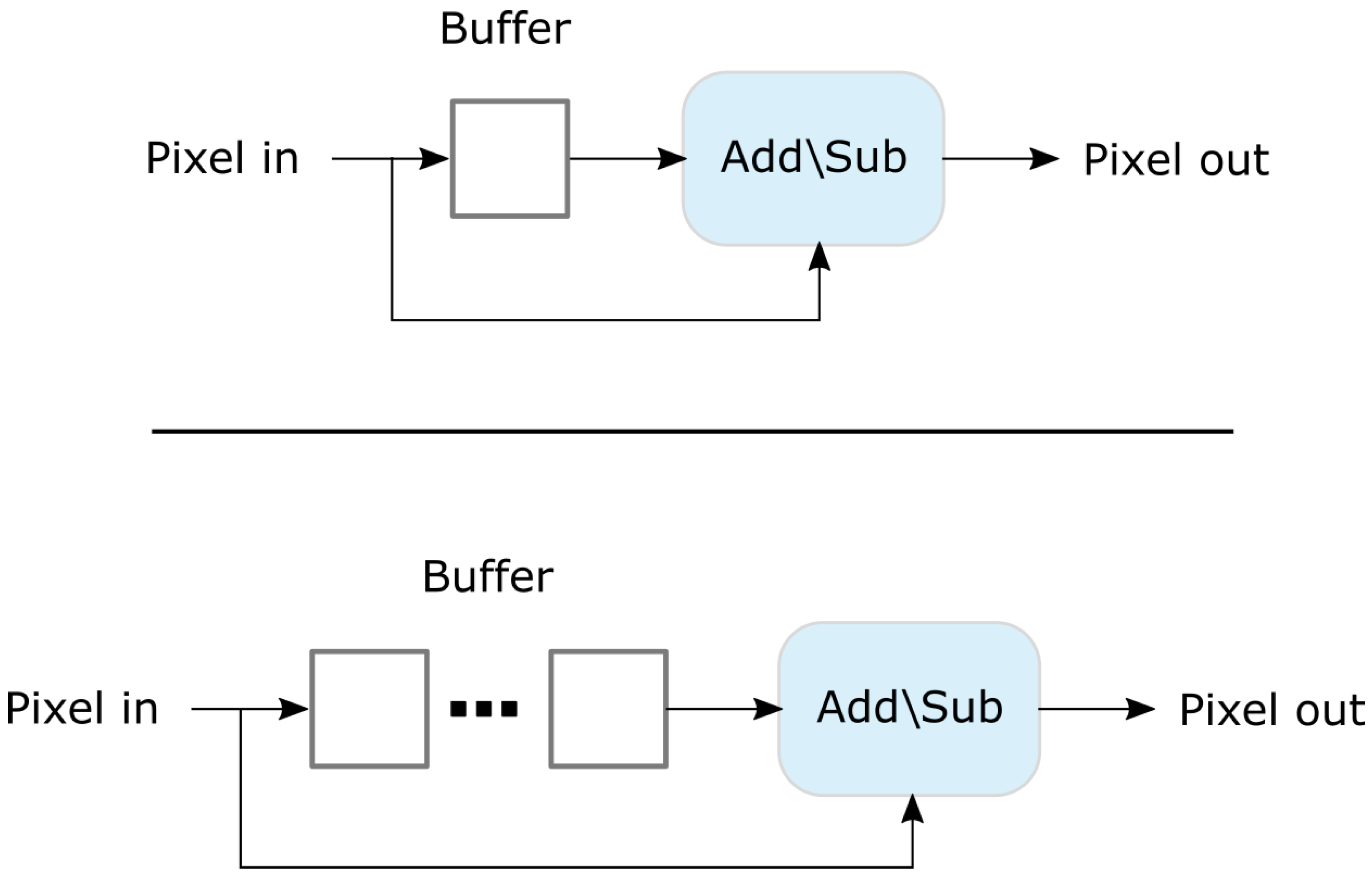
2.2.2. Efficient Calculation

Convolutions with these simple building block kernels require no multiplication, since the kernels only use values of 1 and −1. It is also important to note that the order in which they are applied does not matter. With these building blocks, whole sets of image features can be efficiently calculated.

These convolutions can be fully pipelined in a FPGA or ASIC hardware design with a buffer and an adder/subtract unit. Operations along the axis of the image that is streamed (usually along the x axis) require only a single pixel to be buffered, and operations in the other direction require a single line to be buffered, as shown in Figure 5.

Since all jet features are made of common elements and the order of those operations does not matter, the results of lower order jet features can be used to calculate higher order ones. This makes it very efficient to calculate all jet features up to a certain degree. By forming a lattice of buffers and add/subtraction units, scaling and partial derivative operations can be fed into one another creating sets of jet features.

2.2.3. Multiscale Local Jets

Jet features borrow their name from the concept of multiscale local jets, introduced by Florack et al. [24]. A multiscale local jet is the set of partial derivatives of a given function taken to an nth degree in each dimension. This set is then scaled to various sizes producing a set of transforms that encapsulate useful features at various scales. This is a generalization of the scaling and gradient calculations used in most classic computer vision algorithms. It has been used as a general purpose set of features for image classification, image compression and feature matching [25,26,27].

2.2.4. The ECO Jet Features Algorithm

Jet features were originally developed to make the evolution constructed features (ECO features) algorithm [11] more hardware friendly. The ECO features algorithm uses a grab bag of traditional image transforms and a genetic algorithm (GA) to select, configure and order the transforms into a series, called an ECO features. ECO features are used for image classification.

Many of the original transforms used by the algorithm were not hardware-friendly, making it impractical to implement them in an FPGA. It was observed that the convolutional filters, especially the Sobel and Gaussian filters, were selected most often by the GA. Instead of making hardware units to compute each type of convolution filters, jet features were developed as a set of convolutional filters that could all be easily computed with limited resources. With jet features, the GA determines the number of scaling factors and partial derivatives used in each feature. This variation of the algorithm is called the ECO jet features algorithm and is comparable to the original ECO features algorithms in terms of accuracy in achieving faster execution times on CPUs and easily implemented in an FPGA.

3. Neural Jet Features

In this work, we propose a new binarized convolutional layer called the neural jet features layer. Neural jet features are jet features used in place of standard binarized convolutional filters, trained through deep learning. Neural jet features require fewer parameters and fewer operations than the traditional convolutional layers used in BNNs. They learn essential classic computer vision kernels, combined through deep learning. It is not possible for standard BNN convolutional layers to learn these classic computer vision features. The results in Section 4 show that BNNs using neural jet features achieve comparable accuracy on certain image classification tasks compared to BNNs using binary conventional layers. Convolutions typically account for the majority of operations in a BNN, and by using fewer operations to perform convolution, neural jet features allow BNNs to fit into resource-limited ASICs and FPGAs.

The small $2\times 1$ kernels that make up a jet feature, as shown in Figure 3, differ only in orientation and whether their second element contains a −1 or 1. A $3\times 3$ jet kernel is formed from four of these smaller kernels, thus four binary weights need to be selected to form a $3\times 3$ jet feature.

3.1. Constrained Neural Jet Features

In our previous work on the ECO jet features algorithm [10], we observed that the genetic algorithm selected scaling factors ([1, 1]) more frequently than partial derivatives ([1, −1]) when forming jet features. Based on this observation, we experimented with a constrained version of neural jet features where one of the vertical parameters and one of the horizontal parameters was forced to be 1, forming scaling factors more often than partial derivatives. This reduces the computational cost of neural jet features (Section 3.2) while increasing the average accuracy in some of our testing compared to unconstrained neural jet features (Section 4). With only two binary parameters to be learned per kernel, there are only four possible kernels, the Gaussian kernel, vertical and horizontal Sobel kernels, and a diagonally oriented edge detector, as shown in Figure 2. The constrained version of neural jet features is more efficient than the unconstrained version with comparable or better accuracy. The constrained form of neural jet features is the proposed form of neural jet features.

3.2. Computational Efficiency

Neural jet features learn how to combine input channels using these four classical computer vision kernels, shown in Figure 2. These kernels have been essential to traditional computer vision and are often used multiple times within a single algorithm [22,23]. Since there are only four possible kernels to be learned, it may make more sense to view a neural jet feature layer as a layer that learns to combine these four features with the four features of all the other input layers. Even though there are only four possible features to learn for each input channel, there are $N^4$ unique ways in which to combine the features of the input channels to form a single output channel, where N is the number of input channels.

Like traditional convolutional layers, neural jet features reuse weights in ways that emulate traditional computer vision and image processing. Instead of learning separate weights for every combination of input and output pixel, as done in fully connected layers, convolutional layers form weights into kernels, that are applied locally and reused throughout the entirety of the input image, greatly reducing the number of weights to be learned. Similarly, neural jet features also reuse weights. Neural jet features do not learn unique kernels for each and every combination of input and output channels. Instead, all four $3\times 3$ jet features are applied to each input channel and then reused as needed to form the output channels. This reduces the number of operations required, especially when there are more than just a few output channels.

All four jet features are made up of similar $2\times 1$ convolutions, as shown in Figure 4. Since all four jet features are always calculated for every input channel (and reused as needed), these convolutions can be effectively calculated as a group. The smaller $2\times 1$ convolutions that are common to multiple features can be calculated first and reused to calculate the larger $3\times 3$ jet features. Figure 6 shows how these $2\times 1$ kernels can be applied in an effective manner to reduce the number of operations that are needed. By contrast, four arbitrary $3\times 3$ binary convolutions are not guaranteed to share any common operations, thus they must be calculated independently of each other.

Both of these aspects, kernel reuse and common $2\times 1$ convolutions, make neural jet features computationally efficient compared to standard binary convolutions. These bitwise efficiencies are particularly well suited for FPGA and ASIC implementations where data paths are designed at a bitwise level of granularity.

We illustrate the computational efficiency of neural jet features with a potential FPGA hardware design, shown in Figure 6. This top diagram shows a typical multiply-accumulate operation for an input channel in a BNN. The multiplication operations are simply bitwise XNOR operations. The addition operations are organized into a tree structure to reduce the resources needed. One accumulation tree is required for every output channel. In contrast, the number of accumulation operations in a neural jet feature layer does increase with added output channels. All features are calculated and reused as needed to form the output channels. The addition and subtraction units in the bottom two diagrams are the same units shown in Figure 5.

To form a rough comparison of the computational cost of each of the options shown in Figure 6, we assign a cost of 1, 2, 3 or 4 Full Adder(FA) units to each of the operations depending on the number of bits in their operands. We assign a cost of 2 to the final addition of the standard BNN convolutional layer, which has a 4-bit operand and a 1-bit operand. The standard BNN would cost 13 FAs per output channel. For the unconstrained neural jet features the cost would be 61 FAs to produce all 9 features. The constrained version would only cost 27 FAs for all possible jet features. In layers with 3 or more output channels, calculating all of the constrained jet features is less expensive than standard BNN convolutions. For example, in a layer with 64 output channels, a standard BNN layer would cost 832 FAs ($64\times 13$), while a constrained neural jet feature layer would cost only 27 FAs, since the features would be reused as needed. The number of accumulation resources does not scale the number of output channels like they do in standard BNN convolutional layers. We note that these comparisons are hypothetical, and as part of our future work we plan to implement standard BNN convolutional layers and neural jet feature layers in an FPGA to more accurately demonstrate their computational efficiency.

4. Results

We tested neural jet features on datasets that are representative of visual inspection tasks where the images are of a somewhat consistent scale and/or orientation. We used the BYU Fish dataset [10], BYU Cookie dataset and the MNIST dataset [28]. The MNIST dataset has a bit more variety, which is not typical of visual inspection datasets, but it does lend insight into how jet features compare on a widely used dataset.

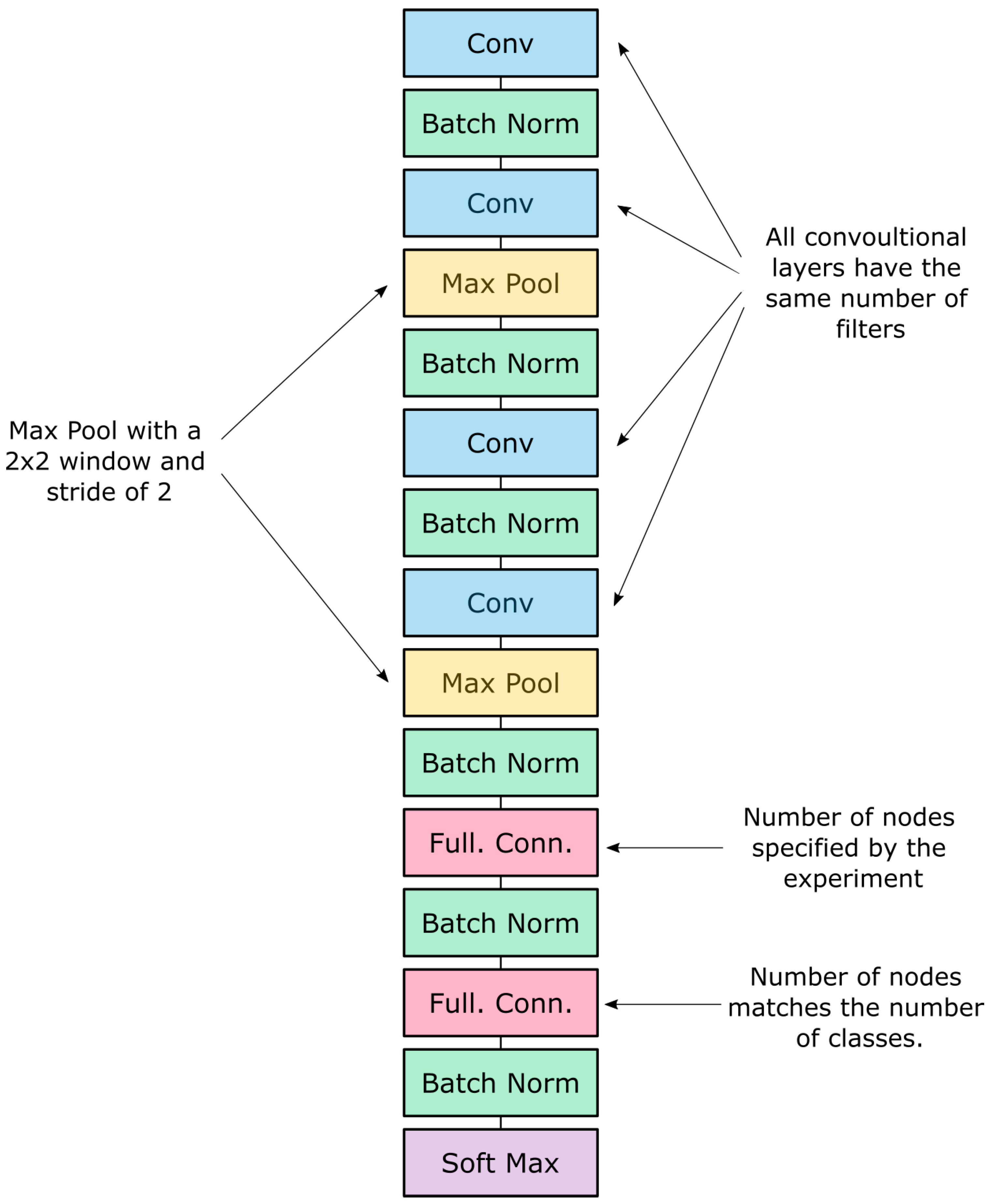
4.1. Model Architecture

We experimented with three different types of convolutional layers: standard binarized convolutional layers [6], unconstrained neural jet feature layers, and constrained neural jet feature layers (see Section 3.1). For all experiments, we used a similar VGG style model topology: Conv-BN- Conv-MP-BN-Conv-BN-Conv-MP-BN-FC-BN-FC-BN-SM (Figure 7), where Conv represents convolutional layers, BN represents batch normalization layers, MP represents max pool layers, FC represents fully connected layers and SM represents a softmax activation with a window of $2\times 2$ and stride of 2, FC represents fully connected layers where the first one contains the number of nodes specified by the experiment and the second one contains the same number of nodes as there are different classes in the dataset being used. The number of filters in the convolutional layers and the number of neurons in the first fully connected layer is specified by the experiment, shown in

Table 1. The layer sizes used for each dataset.

Dataset	Conv. Filters	Fully Connected Units
BYU Fish	8	16
BYU Cookie	8	8
MNIST	16	32
MNIST	32	128
MNIST	64	256

. We note that these models are smaller than most BNNs used throughout the literature [8]. All convolutional layers used the same number of filters for a given experiment. The activation function was the binarization operation that takes place after the batch normalization layers, except after the final batch normalization layer where a softmax function was used. The inputs were not binarized, similar to other BNNs throughout the literature.

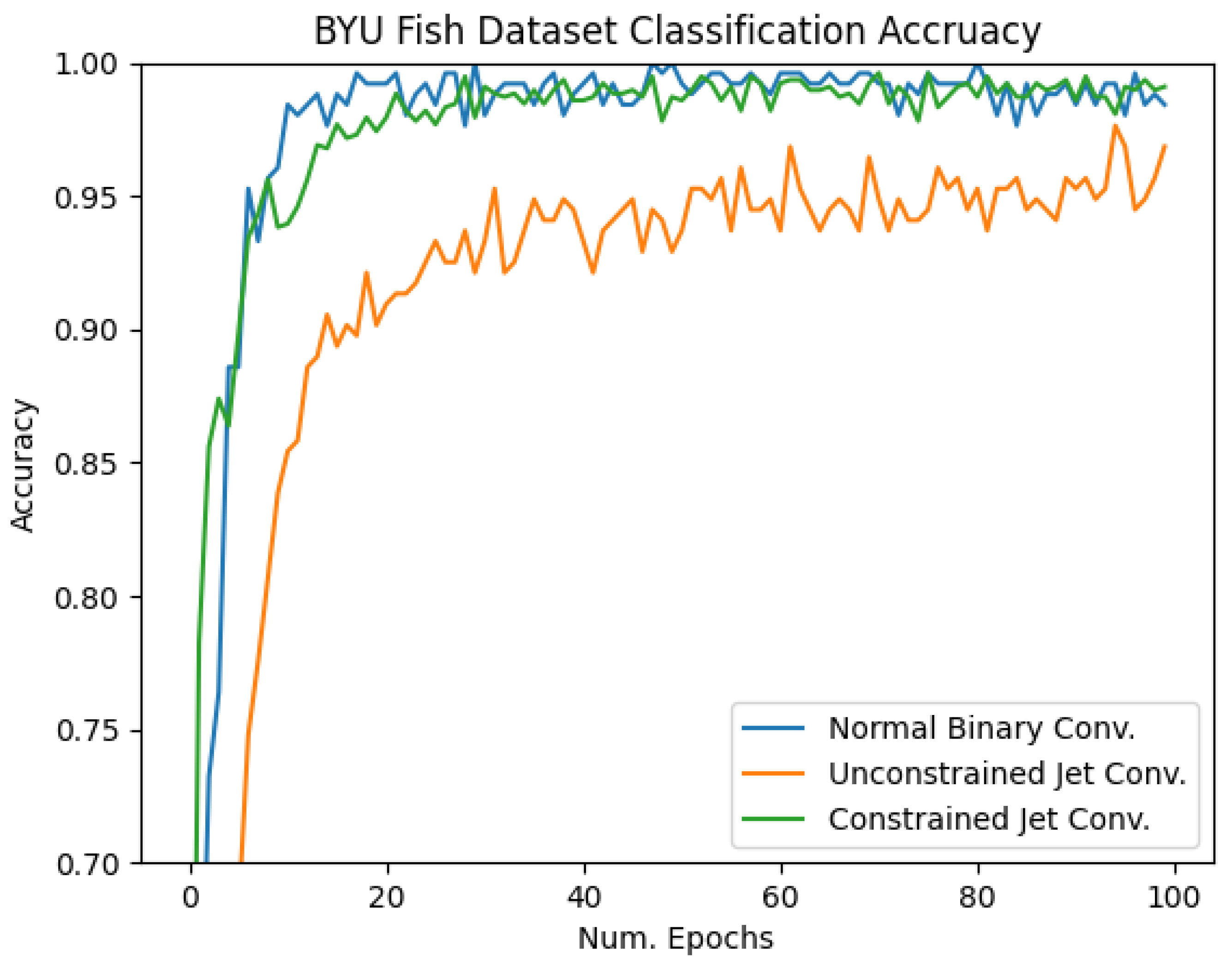
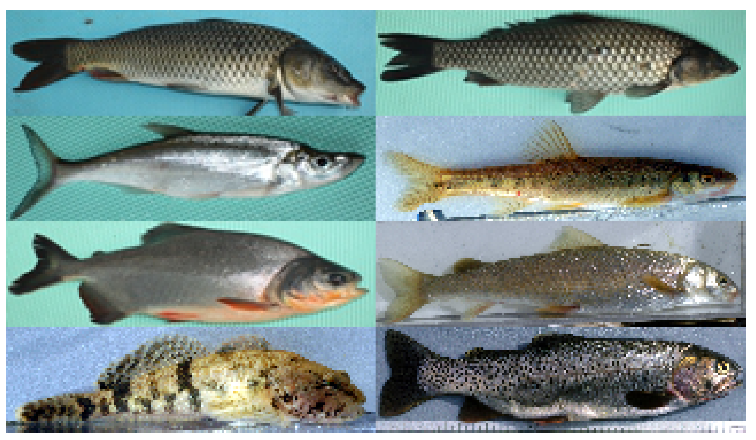
4.2. BYU Fish Dataset

The BYU Fish dataset consists of images of eight different fish species, all oriented the same way, 161 pixels wide and 46 pixels high. Examples are shown in Figure 8. The model used when testing the BYU dataset used eight filters in the convolutional layers and 16 neurons in the fully connected layer.

From the results shown in Figure 9, we see that the standard BNN convolutional layers and the constrained neural jet features performed similarly on the BYU Fish dataset, both reaching an average accuracy of 99.8% accuracy. Unconstrained neural jet features performed worse, hovering around 95% accuracy, significantly worse than the constrained neural jet features. A similar pattern was shown with the BYU Cookie dataset as well, which we hypothesize is due to the fact that the unconstrained neural jet features are allowed to learn features that are not as useful as the one the constrained version learns.

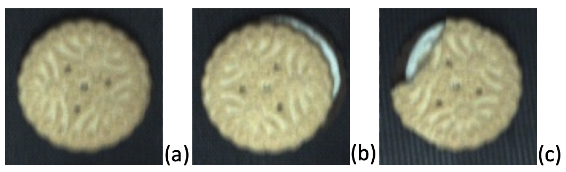
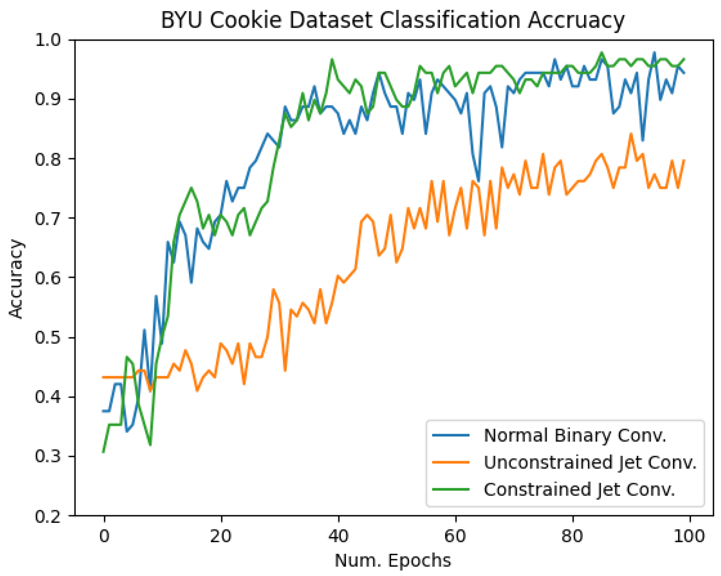
4.3. BYU Cookie Dataset

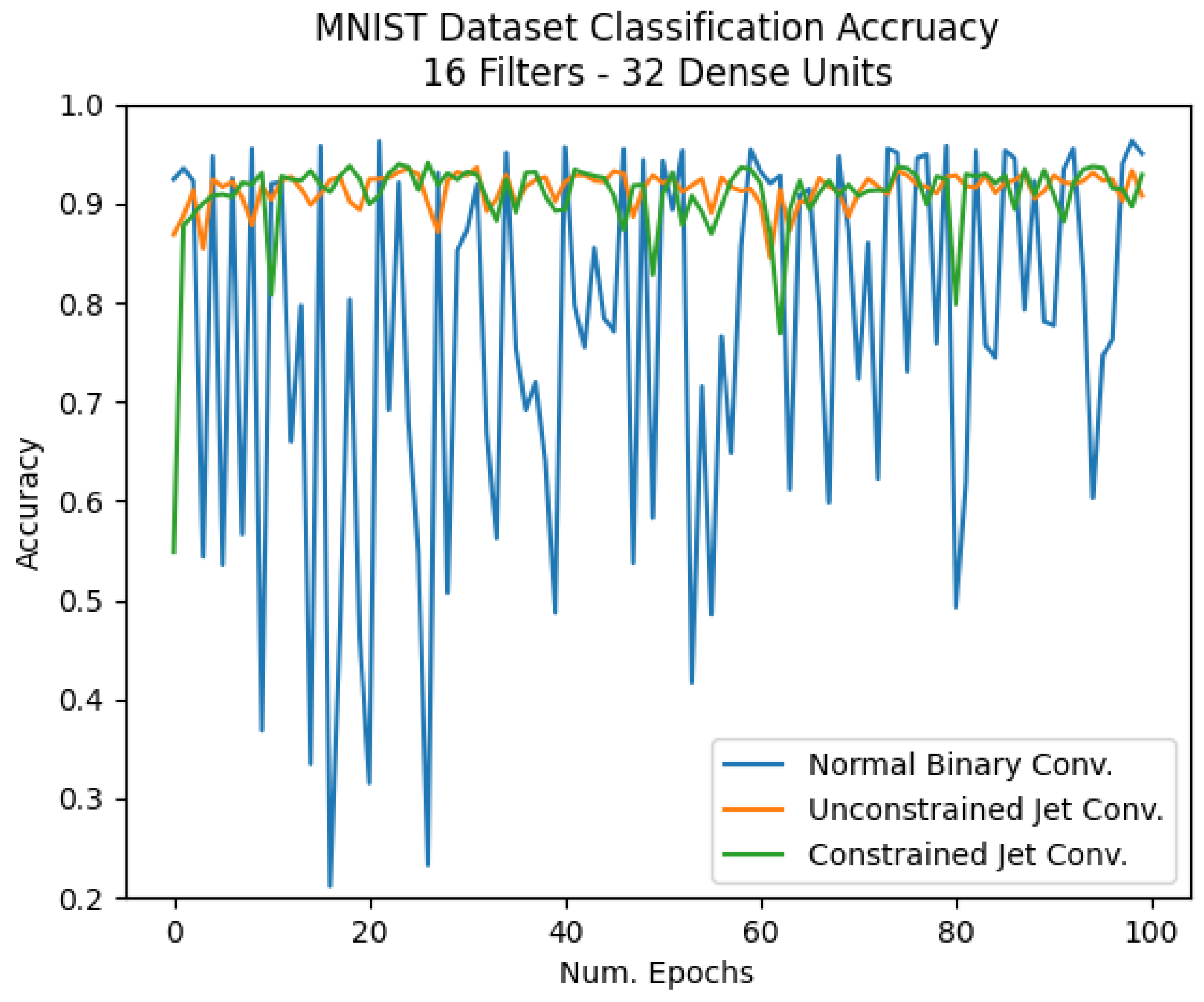
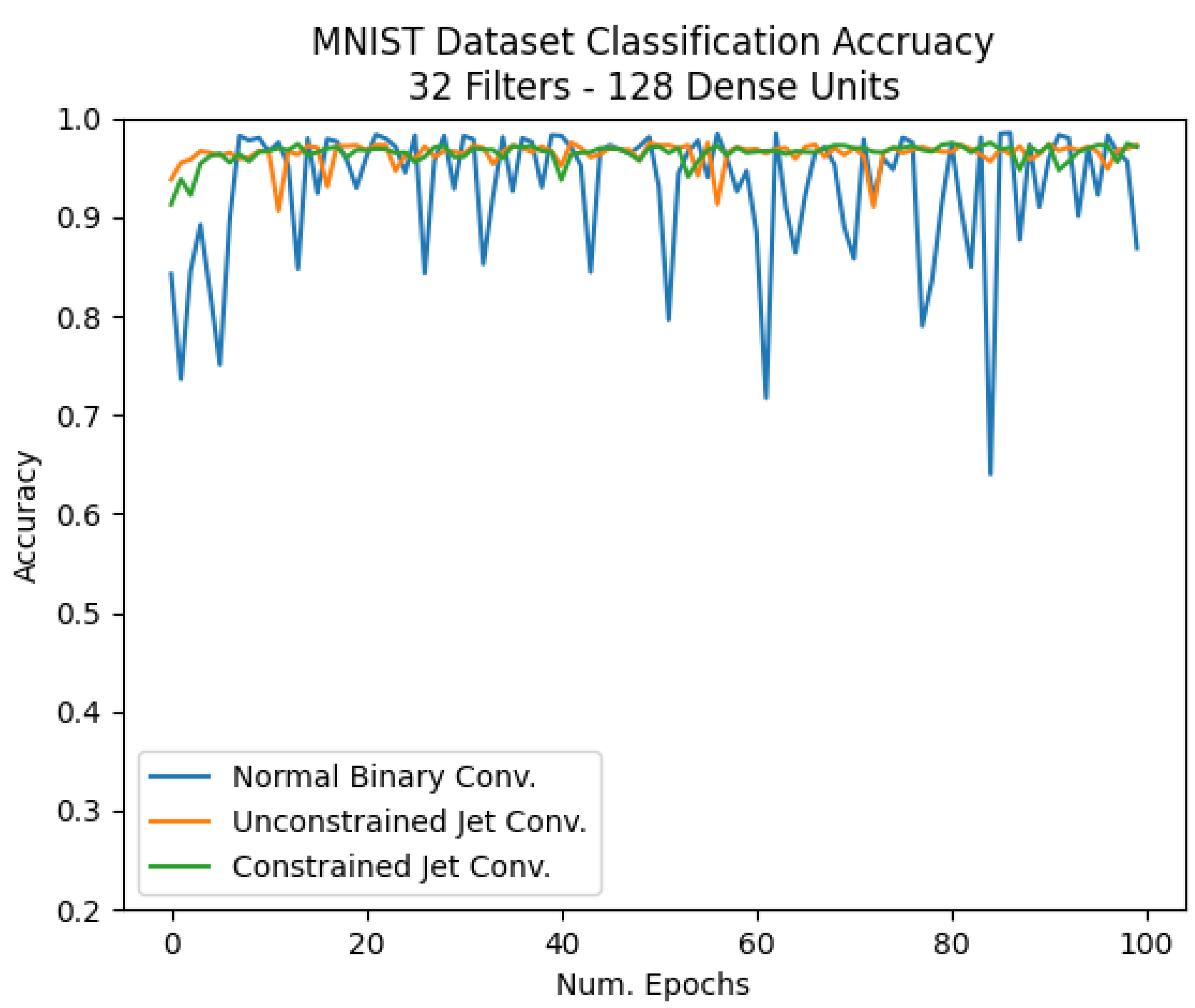
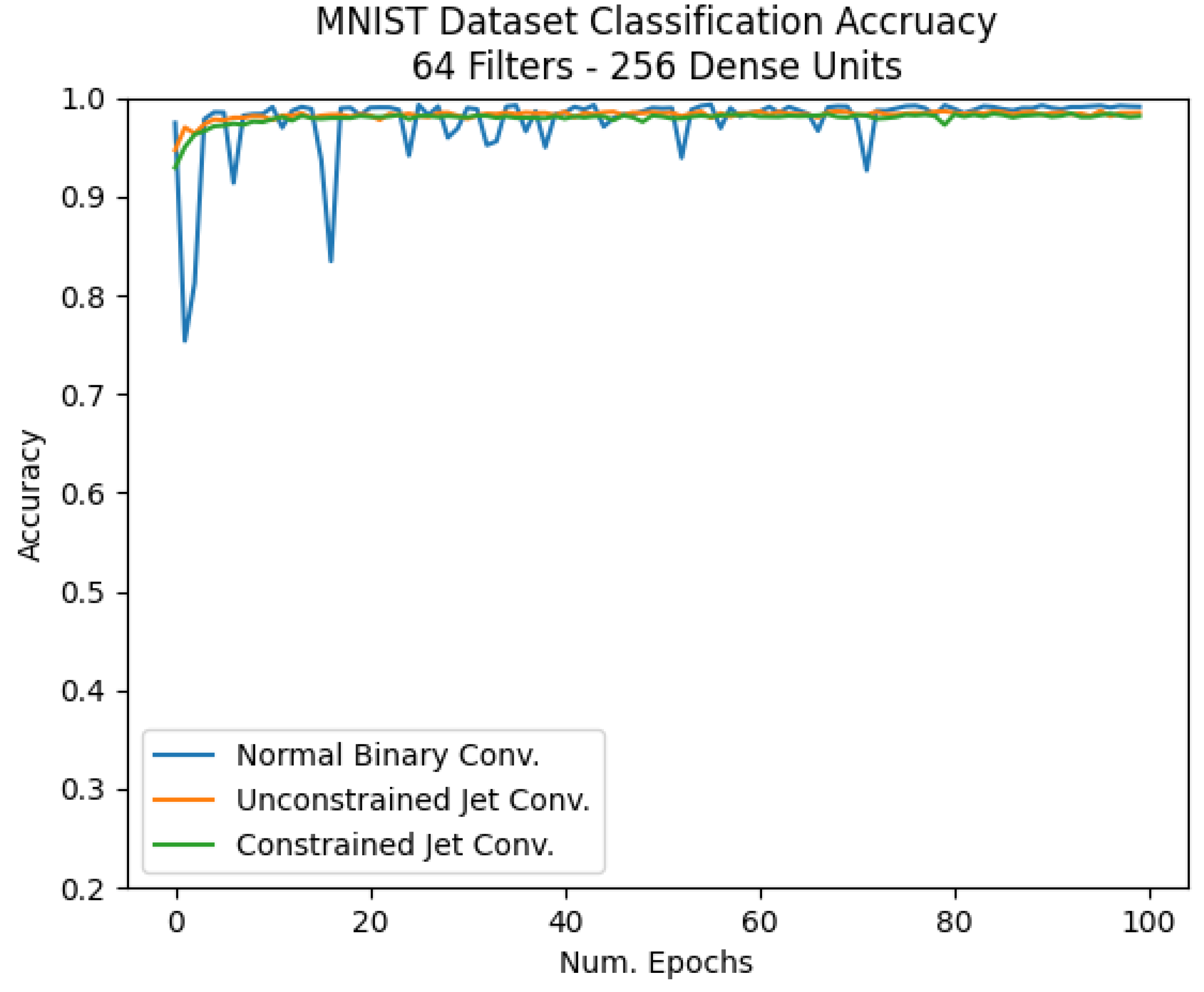
The BYU Cookie dataset includes images of sandwich style cookies that are either in good condition, offset, or broken, as seen in Figure 10. These images are $100\times 100$ pixels in size. This dataset is fairly small, with 345 training images and 88 validation images.

The validation accuracy on the BYU Cookie dataset, shown Figure 11, shows that the normal BNN convolution and constrained Neural jet features outperform unconstrained Neural jet features. In addition, we see that validation accuracy is sporadic over the course of training, which is to be expected when dealing with a smaller dataset. The results seem to be more consistent when using constrained neural jet features than standard BNN convolutional layers, which can also be observed in the results from the MNIST dataset.

4.4. MNIST Dataset

The MNIST dataset consists of 70,000 images of handwritten numbers [28], $28\times 28$ pixels in size. We trained three models of different sizes on this dataset: one model consisting of 16 filters and 32 fully connected units, one with 32 filters and 128 fully connected units and another with 64 filters and 256 fully connected units, which are smaller than other models trained on this dataset [8]. Figure 12, Figure 13 and Figure 14 show the validation accuracy of these models, respectively. The scale of the y-axis is kept consistent between these three figures in order to easily compare the results between each of them. In the larger model, the average accuracy of all models approached 99%.

On the smaller models, the normal BNN convolutions produce inconsistent results, shown in Figure 12 and Figure 13, and as seen on the BYU Cookie dataset. This demonstrates a known difficulty in working with small BNNs. Switching binarized weights between the values −1 and 1 can have dramatic effects in local regions of the network during the learning process. By adding more weights to a model, this effect is mitigated, as seen in Figure 14. Our experiments show that neural jet features are less susceptible to this effect, making them a good choice for smaller BNN models. We postulate that this is due to the fact that Neural jet feature convolutional layers are limited to the classic computer vision kernels shown in Figure 2.

4.5. Comparison and Discussion

Table 2. Performance comparison.

Dataset	Normal Binary Conv.	Unconstrained Jet Conv.	Constrained Jet Conv.
BYU Fish	99.8%	95%	99.8%
BYU Cookie	95%	77.5%	96%
MNIST 16 Filters	93%	92%	92%
MNIST 32 Filters	92%	97%	97%
MNIST 64 filters	99%	98%	98%

summarizes the performance of these three methods on all three datasets after 100 epochs of training. Although the final accuracies for the normal binary convolution and constrained jet convolution are comparable for the BYU Fish dataset and MNIST dataset using 16 and 64 filters, constrained jet convolution had much more stable performance as shown in Figure 9, Figure 11, Figure 12, Figure 13 and Figure 14.

5. Conclusions

We have presented neural jet features, a binarized convolutional layer that combines the power of deep learning with classic computer vision kernels. Not only do neural jet features require fewer operations than standard convolutional layers in BNN’s, but they are also more stable in smaller models that would be used for visual inspection tasks. Neural jet features have comparable accuracy on visual inspection datasets while requiring fewer operations and parameters. Neural jet features offer an efficient solution for resource-limited systems that can take advantage of their bitwise efficiency, like ASIC and FPGA designs. Future work includes implementing a BNN on an FPGA using neural jet features to measure logic resource savings. We also plan on exploring the use of neural jet features in various state-of-the-art topologies like attention-based models [29] and skip-connection-based models [30].

References

1. Iandola, F.N.; Moskewicz, M.W.; Ashraf, K.; Han, S.; Dally, W.J.; Keutzer, K. SqueezeNet: AlexNet-level accuracy with 50x fewer parameters and <1 MB model size. arXiv 2016, arXiv:1602.07360. [Google Scholar]
2. Hanson, S.J.; Pratt, L. Comparing Biases for Minimal Network Construction with Back-propagation. In Advances in Neural Information Processing Systems 1; Morgan Kaufmann Publishers Inc.: San Francisco, CA, USA, 1989; pp. 177–185. [Google Scholar]
3. Cun, Y.L.; Denker, J.S.; Solla, S.A. Optimal Brain Damage. In Advances in Neural Information Processing Systems 2; Morgan Kaufmann Publishers Inc.: San Francisco, CA, USA, 1990; pp. 598–605. [Google Scholar]
4. Han, S.; Mao, H.; Dally, W.J. Deep Compression: Compressing Deep Neural Network with Pruning, Trained Quantization and Huffman Coding. arXiv 2015, arXiv:1510.00149. [Google Scholar]
5. Han, K.; Wang, Y.; Tian, Q.; Guo, J.; Xu, C.; Xu, C. GhostNet: More Features from Cheap Operations. 2020. Available online: https://arxiv.org/abs/1911.11907 (accessed on 17 June 2021).
6. Courbariaux, M.; Bengio, Y. BinaryNet: Training Deep Neural Networks with Weights and Activations Constrained to +1 or -1. arXiv 2016, arXiv:1602.02830. [Google Scholar]
7. Russakovsky, O.; Deng, J.; Su, H.; Krause, J.; Satheesh, S.; Ma, S.; Huang, Z.; Karpathy, A.; Khosla, A.; Bernstein, M.; et al. ImageNet Large Scale Visual Recognition Challenge. Int. J. Comput. Vis. IJCV 2015, 115, 211–252. [Google Scholar] [CrossRef] [Green Version]
8. Simons, T.; Lee, D.J. A Review of Binarized Neural Networks. Electronics 2019, 8, 661. [Google Scholar] [CrossRef] [Green Version]
9. Qasaimeh, M.; Denolf, K.; Lo, J.; Vissers, K.; Zambreno, J.; Jones, P.H. Comparing Energy Efficiency of CPU, GPU and FPGA Implementations for Vision Kernels. In Proceedings of the 2019 IEEE International Conference on Embedded Software and Systems (ICESS), Las Vegas, NV, USA, 2–3 June 2019; pp. 1–8. [Google Scholar]
10. Simons, T.; Lee, D.J. Jet features: Hardware-Friendly, Learned Convolutional Kernels for High-Speed Image Classification. Electronics 2019, 8, 588. [Google Scholar] [CrossRef] [Green Version]
11. Lillywhite, K.; Tippetts, B.; Lee, D.J. Self-tuned Evolution-COnstructed features for general object recognition. Pattern Recognit. 2012, 45, 241–251. [Google Scholar] [CrossRef]
12. Bulat, A.; Tzimiropoulos, G. Binarized Convolutional Landmark Localizers for Human Pose Estimation and Face Alignment with Limited Resources. In Proceedings of the 2017 IEEE International Conference on Computer Vision (ICCV), Venice, Italy, 22–29 October 2017; pp. 3726–3734. [Google Scholar]
13. Bengio, Y.; Léonard, N.; Courville, A. Estimating or Propagating Gradients Through Stochastic Neurons for Conditional Computation. 2013. Available online: https://arxiv.org/abs/1308.3432 (accessed on 17 June 2021).
14. Rastegari, M.; Ordonez, V.; Redmon, J.; Farhadi, A. XNOR-Net: ImageNet Classification Using Binary Convolutional Neural Networks. In Proceedings of the European Conference on Computer Vision (ECCV), Amsterdam, The Netherlands, 11–14 October 2016; pp. 525–542. [Google Scholar]
15. Zhou, S.; Ni, Z.; Zhou, X.; Wen, H.; Wu, Y.; Zou, Y. DoReFa-Net: Training Low Bitwidth Convolutional Neural Networks with Low Bitwidth Gradients. arXiv 2016, arXiv:1606.06160. [Google Scholar]
16. Lin, X.; Zhao, C.; Pan, W. Towards Accurate Binary Convolutional Neural Network. NIPS. 2017. Available online: https://arxiv.org/abs/1711.11294 (accessed on 17 June 2021).
17. Zhao, R.; Song, W.; Zhang, W.; Xing, T.; Lin, J.H.; Srivastava, M.; Gupta, R.; Zhang, Z. Accelerating Binarized Convolutional Neural Networks with Software-Programmable FPGAs. In Proceedings of the 2017 ACM/SIGDA International Symposium on Field-Programmable Gate Arrays—FPGA ’17; ACM Press: New York, NY, USA, 2017; pp. 15–24. [Google Scholar]
18. Guo, P.; Ma, H.; Chen, R.; Li, P.; Xie, S.; Wang, D. FBNA: A Fully Binarized Neural Network Accelerator. In Proceedings of the 2018 28th International Conference on Field Programmable Logic and Applications (FPL), Dublin, Ireland, 27–31 August 2018; pp. 51–513. [Google Scholar]
19. Fraser, N.J.; Umuroglu, Y.; Gambardella, G.; Blott, M.; Leong, P.; Jahre, M.; Vissers, K. Scaling Binarized Neural Networks on Reconfigurable Logic. In Proceedings of the 8th Workshop and 6th Workshop on Parallel Programming and Run-Time Management Techniques for Many-core Architectures and Design Tools and Architectures for Multicore Embedded Computing Platforms—PARMA-DITAM ’17; ACM Press: New York, NY, USA, 2017; pp. 25–30. [Google Scholar]
20. Ghasemzadeh, M.; Samragh, M.; Koushanfar, F. ReBNet: Residual Binarized Neural Network. In Proceedings of the 2018 IEEE 26th Annual International Symposium on Field-Programmable Custom Computing Machines (FCCM), Boulder, CO, USA, 29 April–1 May 2018; pp. 57–64. [Google Scholar]
21. Umuroglu, Y.; Fraser, N.J.; Gambardella, G.; Blott, M.; Leong, P.; Jahre, M.; Vissers, K. FINN. In Proceedings of the 2017 ACM/SIGDA International Symposium on Field-Programmable Gate Arrays—FPGA ’17; ACM Press: New York, NY, USA, 2017; pp. 65–74. [Google Scholar]
22. Lowe, D.G. Distinctive Image Features from Scale-Invariant Keypoints. Int. J. Comput. Vis. 2004, 60, 91–110. [Google Scholar] [CrossRef]
23. Bay, H.; Tuytelaars, T.; Van Gool, L. SURF: Speeded Up Robust Features. In Computer Vision—ECCV 2006; Leonardis, A., Bischof, H., Pinz, A., Eds.; Springer: Berlin/Heidelberg, Germany, 2006; pp. 404–417. [Google Scholar]
24. Florack, L.; Ter Haar Romeny, B.; Viergever, M.; Koenderink, J. The Gaussian Scale-space Paradigm and the Multiscale Local Jet. Int. J. Comput. Vision 1996, 18, 61–75. [Google Scholar] [CrossRef]
25. Lillholm, M.; Pedersen, K.S. Jet based feature classification. In Proceedings of the 17th International Conference on Pattern Recognition ICPR 2004, Cambridge, UK, 26 August 2004; Volume 2, pp. 787–790. [Google Scholar]
26. Larsen, A.B.L.; Darkner, S.; Dahl, A.L.; Pedersen, K.S. Jet-Based Local Image Descriptors. In Computer Vision—ECCV 2012; Fitzgibbon, A., Lazebnik, S., Perona, P., Sato, Y., Schmid, C., Eds.; Springer: Berlin/Heidelberg, Germany, 2012; pp. 638–650. [Google Scholar]
27. Manzanera, A. Local jet feature Space Framework for Image Processing and Representation. In Proceedings of the 2011 Seventh International Conference on Signal Image Technology Internet-Based Systems, Dijon, France, 28 November–1 December 2011; pp. 261–268. [Google Scholar]
28. Lecun, Y.; Bottou, L.; Bengio, Y.; Haffner, P. Gradient-based learning applied to document recognition. Proc. IEEE 1998, 86, 2278–2324. [Google Scholar] [CrossRef] [Green Version]
29. Vaswani, A.; Shazeer, N.; Parmar, N.; Uszkoreit, J.; Jones, L.; Gomez, A.N.; Kaiser, L.u.; Polosukhin, I. Attention is All you Need. In Advances in Neural Information Processing Systems; Guyon, I., Luxburg, U.V., Bengio, S., Wallach, H., Fergus, R., Vishwanathan, S., Garnett, R., Eds.; Curran Associates, Inc.: Red Hook, NY, USA, 2017; Volume 30. [Google Scholar]
30. He, K.; Zhang, X.; Ren, S.; Sun, J. Deep Residual Learning for Image Recognition. In Proceedings of the 2016 IEEE Conference on Computer Vision and Pattern Recognition (CVPR), Las Vegas, NV, USA, 26 June–1 July 2016; pp. 770–778. [Google Scholar]
Figure 1. Visualization of a binarization layer in a BNN. Real valued weights are stored behind a binarization layer. During the forward pass, these real valued weights are binarized and passed forward through the network. During the backward pass, the gradients bypass the binarization layer, and instead are passed through a straight through estimator and used to update the real valued weights.
Electronics 10 01511 g001
Figure 2. The classic computer vision kernels that can be constructed with “constrained” neural jet features (see Section 3.1).
Electronics 10 01511 g002
Figure 3. The 2 × 1 kernels that are used to form jet features.
Electronics 10 01511 g003
Figure 4. Examples of how jet feature building blocks can be applied through successive convolutions to implement classic computer vision kernels.
Electronics 10 01511 g004
Figure 5. Line buffers and arithmetic operations used to form jet feature building blocks. A single pixel buffer (top) is used to compute jet building block operations in the x direction and a line buffer (bottom) is used to compute operations in the y direction. Addition is used for scaling factors and subtraction is used for partial derivatives.
Electronics 10 01511 g005
Figure 6. An example of how the operations in neural jet features can be arranged. The number of operations to calculate all features in a standard BNN convolutional layer scales with the number of output channels. For neural jet feature layers, the number of operations to calculate the features is the same regardless of how many output channels there are.
Electronics 10 01511 g006
Figure 7. The model topology used for all experiments. The number of filters in the convolutional layers and the number of nodes in the first fully connected layer change per experiment.
Electronics 10 01511 g007
Figure 8. Examples from the BYU Fish dataset. The images in this dataset are 161 × 46 of eight different fish species.
Electronics 10 01511 g008
Figure 9. Classification accuracy on the BYU Fish dataset.
Electronics 10 01511 g009
Figure 10. Examples from the BYU Cookie Dataset. The images in this dataset are 100 × 100 pixels from three classes, (a) good, (b) offset, or (c) broken.
Electronics 10 01511 g010
Figure 11. Classification accuracy on the BYU Cookie dataset.
Electronics 10 01511 g011
Figure 12. Classification accuracy on the MNIST dataset with 16 filters and 32 dense units.
Electronics 10 01511 g012
Figure 13. Classification accuracy on the MNIST dataset with 32 filters and 128 dense units.
Electronics 10 01511 g013
Figure 14. Classification accuracy on the MNIST dataset with 64 filters and 256 dense units.
Electronics 10 01511 g014